
Abstract
In this paper, controller tuning methods based on stability region centroid methods reported in the literature are used to design PI-PD controllers for unstable, integrating and resonant systems with time delay. By analyzing the stability boundary locus (SBL) for the PD controller, which is utilized in the inner loop of this structure, the controller parameters are obtained using three methods which are the Weighted Geometric Center (WGC), Centroid of Convex Stability Region (CCSR), and Stability Triangle Approach (STA). These techniques were applied analytically, step by step. For the closed loop transfer function obtained in the inner loop of the controlled system, these three methods were utilized to design the PI controller in the outer loop, individually. Unit step responses of the controlled system, using PI-PD gains determined by each method, have been obtained. Furthermore, a disturbance of a certain time and amplitude was added to the systems to test the disturbance rejection behavior and the robustness performance of the methods. Perturbed responses were obtained through changing the model parameters at a certain rate. Time domain performance metrics were analyzed to compare the responses. The simulations were evaluated using settling time, rise time, and percentage overshoot as the assessment criteria. As a result of this study, the effectiveness of three methods, namely WGC, CCSR, and STA, in controller design for unstable, integrating, and resonant time-delay systems has been demonstrated. In addition, a comparison of time domain performance metrics is presented for the nominal and perturbed systems. Based on these comparisons, it is concluded that the methods outperform each other only in some time response performance measures. The presented results showed the advantages of these methods over each other in terms of some performance criteria. The contribution of this study to the literature is the comparative analysis of these three analytical methods.
Keywords
Introduction
Despite significant advancements in control theory, the industrial sector still relies heavily on Proportional-Integral (PI) and Proportional-Integral-Derivative (PID) controllers due to their reliable performance and uncomplicated design. 1 This is mainly because, despite their simple structure, they exhibit robustness in various control systems. 2 The most well-known and established techniques for tuning the controllers are the Ziegler and Nichols, Åström and Hägglund, Cohen and Coon, and Tyreus and Luyben methods. These methods propose using the open-loop unit step response of the system for tuning.3–6 The frequency response analysis-based tuning rule developed by Tyreus and Luyben 5 shows superior performance for systems with a low dead time constant ratio. Smith and Corripio 7 put forward tuning rules using the direct synthesis design method. The Ziegler-Nichols (ZN) method, based on the Nyquist curve, does not provide adequate information about the dynamic behavior of systems. Consequently, it is not suitable for tuning and frequently yields unsatisfactory outcomes. 6 The Åström-Hägglund and subsequent improved ZN techniques have been routinely used in industry and literature for several years due to their simplicity and ease of application.6,8 Although the controller parameters of classical PID controllers can be efficiently determined using these methods, they cannot always provide optimum performance for more complicated systems with non-linear dynamics and time delay. 9 Since unstable systems have poles in the right half s-plane and integrating systems have poles at the origin, the responses of unstable and integrating type systems are prone to uncontrollable oscillations and respond slowly to input adjustments. Therefore, these systems controls are more difficult to than stable processes. 10 In addition, industrial systems are often characterized by time delay, which can complicate these problems by causing additional instability and oscillations. 9 Therefore, traditional PI or PID controllers on its own is insufficient for controlling time-delay, unstable, non-minimum phase, integrating systems and systems with poorly placed complex poles due to its inherent limitations and has poor closed-loop performance in such systems.2,11,12 Even in Unstable First-Order Plus Time-Delay (UFOPTD) systems, a simple PID controller will not provide the desired control performance. 12 For these reasons, the literature suggests that double-loop control schemes are more appropriate for such systems.9,10,13–20 The use of a PI-PD controller as double-loop control schemes can lead to improved control system performance. 21 Using an inner loop featuring a PD controller within the control system has the capability of converting an unstable open-loop system into a stable open-loop system. This can be achieved by providing appropriate placements for the open-loop system poles, which in turn stabilize resonant or integrating systems. 19 The PI controller is used to control the inner loop transfer function with PD feedback and to achieve the desired closed loop performance, following appropriate pole placement. Compared to traditional PI/PID controllers, the PI-PD controller has four adjustable parameters: K f , K d , K p , and K i , making it a superior option.9,18,22,23 However, improper selection of these parameters will result in poor closed-loop performance. Hence, the tuning of these controllers can be accomplished by implementing diverse theoretical methodologies outlined in the literature for unstable, integrating and resonant systems with time delay. However, in systems with large dead time, these control structures alone cannot provide a good servo response.20,24 To overcome this limitation, researchers proposed various dead time compensator designs.12,20,24–26 Rao and Chidambaram 26 designed a modified dead time compensator with three controllers by Direct Synthesis (DS) method to control the processes involving unstable, non-minimum phase with time-delay. PI-PD controller is used for reference input tracking and PID controller in series with a lead-lag filter to reject load disturbance. Another controller the dead time compensator design using the DS method to control unstable, time-delay processes was made by Ajmeri and Ali. 25 PID controller in cascade with a lead-lag compensator is used in the inner loop used for reference input tracking and rejecting load disturbance and PI control is used in the outer loop. The third controller was used to stabilize the non-delayed part of the process model. Another PI-PD controller scheme is proposed by Raja 20 for unstable/integrating plants with time delay and non-minimum phase. The controller has a simple PI-PD based structure and includes a dead time compensator. In his work, Raja proposed a method to obtain PD controller parameters using a combination of Routh stability criteria and maximum sensitivity considerations. PI controller parameters were obtained with the moment matching technique proposed by Raja and Ali. 27 Considering these studies, it seems that appropriate setting of the controllers in the dead time compensator can further increase the performance of the control system. However, the fact that these compensators require more parameter settings makes the use of a simpler control structure more suitable in practical applications. 20 In addition, in PI-PD control structure, a large dead time causes the sluggish output response. To avoid this limitation, the authors used a filter transfer function in inner loop with PD controller in practical applications. 14 Recently, Irshad and Ali 15 proposed a robust PI-PD control structure using the modified integral of the squared error (ISE) criterion and Particle Swarm Optimization to control integrating and unstable processes. The paper published by Kaya, 17 for integrating with dead time processes, a PI–PD controller is designed with simple parameter tuning rules. The integral of squared time 3 error (IST 3 E) criterion was used to calculate the optimum setting parameters and the Particle Swarm Optimization (PSO) was employed to determine PI–PD parameters that minimized the error. Most recently, a dual-degree of freedom PI-PD controller is developed by Das et al. 14 for integrating with dead time chemical processes. The PD controller is designed for inner-loop based on user-defined gain and phase margin. The PI controller is designed for outer loop with maximum sensitivity specifications and using the moment-matching method. Cokmez and Kaya 13 suggested the analytical tuning rules for an optimal I-PD controller based on time-weighted integral performance criteria to reject disturbances for open-loop unstable processes. However, since there is no proportional gain in the I-PD controller type, there is a slowdown in servo tracking. 2 In addition, fractional order controller design is also recommended for time-delay systems in the literature.28,29 Mehta et al. 28 introduced a fractional order integral derivative controller (FOIλD1−λ) for integrating with time-delay plants. The introduced controller contains only three tuning parameters like traditional PIDs. Once the stability region in the controller parameter space was identified through Complex Root Boundary (CRB) analysis, the controller parameters were determined through a three-stage optimization process using the integral squared time error (ISTE) criteria. Mondal and Dey introduced a novel and simplified specification-driven design methodology for enhancing the performance of time delay systems. Their suggestion involves introducing the fractional-order PIλ−PDμ controller and its cascaded form, fractional-order [PI]λ−[PD]μ controller, with the aim of enhancing system performance. 29
The main objective of controller design is to obtain a stable closed-loop transfer function. Therefore, obtaining the stability region of the controller parameters that makes the closed-loop transfer function stable has been one of the most studied topics in recent years. In the literature, there are many studies on finding the region of stability of all PI/PID controller parameters that makes the closed-loop transfer function stable. These are methods based on Hermite-Biehler theorem, 30 parameter space method, 31 Kronecker summation method, 32 and stability boundary locus (SBL) method. 33 The SBL method, introduced by Tan, 21 is a graphical method that determines the stability boundary of the (K p , K i ) parameters that make a closed-loop system stable. The SBL offers an effective solution for certain types of systems and is based on plotting coordinate points in the frequency domain of controller parameters that render closed-loop control stable. This approach facilitates the calculation of PI controller parameters that ensure system stability. Furthermore, the method introduced allows a PI controller to be designed to achieve the gain and phase margins specified by the user. In addition, analytical calculation that finds all the stable values of a PID controller’s parameters is given in the (K p , K i ) plane for a fixed K d , (K p , K d ) plane for a fixed K i , and (K i , K d ) plane for a fixed K p . It has been shown that for a fixed K p value, the convex polygon’s stability boundary at the (K i , K d ) plane can be produced from four straight lines. The equations related to the four straight lines can be obtained using the SBL of the stability regions obtained in the (K p , K i ) plane and in the (K p , K d ) plane. Recently, there has been an increase in research focusing on PID tuning methods based on the stability region.18,19,21,33–48 Similar to the one in Tan, 21 Tan and Atherton 43 applied the SBL method to calculate all the compensating PI controllers for multi-input multiple-output (MIMO) control systems, considering the two-input two-output (TITO) systems. Similarly, the method is used to calculate all stable PI controllers to obtain user-defined gain and phase margins. Also, the method has been extended to handle 3-parameter PID controllers. Tan 42 suggests a technique using plotting the SBL along with the Kharitonov theorem 49 and designing a PI-PD controller for systems with uncertain parameters. Hanwate and Hote applied the SBL method to the control structure containing two PID controllers to stabilize the inverted pendulum system. 50 Kaya and Atıç 36 presented a generalized method to obtain all stabilizing PI controllers. For this purpose, a stable FOPDT model was used to model high-order real plant transfer functions. Thus, there is no need to recalculate SBL in case of different plant transfer functions. If the process transfer function parameters are estimated perfectly, the resulting boundary curves reach exact solutions. Demiroglu et al. 51 presented a systematic design procedure to stabilize PIλ controllers based on the SBL method for tuning in the desired frequency ranges for FOPTD plants. Additionally, instead of testing the stable/unstable regions of the SBL with randomly selected points, it ensures stability with analytically obtained formulas. Chen et al. 52 proposed FOPIλD design method to achieve both time domain requirement and frequency domain specifications. In order to provide frequency domain properties, the authors obtained the FOPIλD controller parameter region with certain phase margin (φ) and gain margin (A) limits with the help of SBL and presented a robust design method for FOPTD systems.
Within the SBL region, there exists an infinite number of controller parameter combinations which make the closed-loop stable. However, any controller parameter value obtained within the SBL region may provide a better time response compared to an any other parameter value. Therefore, identifying suitable points for controller parameters that meet the desired performance criteria within the SBL region has been a widely studied topic in the literature. These methods are characterized as techniques that ensure optimal time-domain properties within the SBL and provide only a single optimal point value. However, as mentioned above, an infinite number of controller parameters can be selected under the SBL. Hence, instead of just a single point under the SBL, a region mapping study has been conducted to identify a region that satisfies some time-domain and frequency-domain properties. 53 Onat 37 introduces an approach to computing PI controller parameters for time-delay systems, based on SBL. The method involves obtaining PI parameters by determining the Weighted Geometric Center (WGC) of the stable controller region. To calculate the WGC in the stable region, the coordinate points of the boundary of the SBL are utilized. Ozyetkin et al. 19 have presented a simple tuning method for PI-PD controllers for time delay systems via WGC. Onat et al. 48 presented a PI-PD controller design procedure for magnetic levitation systems. The proposed method is based on obtaining the stable region for the controller parameters by the SBL method and then calculating the WGC of this region. Güler and Kaya 45 presented the PI-PD controller, a robust and disturbance rejection capable design based on the WGC of the stability region, for load frequency control of a single area single or multi source power system. Most recently, Cetintas et al. 54 suggested finding the PID stability region using the SBL method for time-delay systems and appropriate PID adjustment with the WGC method. After determining the K d stability parameter range in the (K d , K p ) plane, the authors obtained all stability regions in the (K p , K i ) plane by using these K d values and thus created the three-dimensional (K p , K i , K d ) parameter stability region. Here, they proposed optimum PID tuning by calculating the WGC points of each (K p , K i ) plane. In the literature, the SBL method has also been used for control of fractional order systems and fractional order controller design.39,46 The WGC method was applied by Ozyetkin 39 for integer and fractional order design of PI-PD controllers. This study is based on obtaining stability regions drawn in the (K f , K d ) and (K p , K i ) planes and then calculating the WGCs of these regions.
There are situations where the WGC method is not applicable. 39 If the stabilizing controller parameters vary according to different design cases, the WGC point may fall outside the SBL, in which case the method should be ignored. Furthermore, all frequency-dependent points that form the SBL must be included in the WGC design procedure to calculate the WGC point, leading to a substantial computational load. To address this issue, Onat 18 proposes an approach: the Centroid of the Convex Stability Region (CCSR), for refining the PI-PD parameters of unstable time-delay systems. This method establishes the domain of stable controller parameters by using the coordinates of certain points that belong to the SBL. In the PI controller example, two of the points correspond to where the CRB curve intersects the Real Root Boundary (RRB) line K i = 0. The third point is where K i max reaches its maximum value. Analytically, the centroid of the stable controller parameters and the appropriate controller parameters of the region can be determined. In addition, the computational load of the design procedure is comparatively lower than that of the WGC method, since not all frequency-dependent points are utilized, as in the case of the WGC method. Moreover, the method was applied on a real-time experimental example and its effectiveness in practice was demonstrated. The suggested method also provides stability when the region is tilted and can be applied to all processes where the stability region can be calculated as a closed region. Another significant advantage is the method’s capacity to extend to uncertain plants through the application of the Kharitonov theorem. Zheng et al. 46 proposed a method for unstable time delay and fractional systems to adjust PI-PD parameters using the inner center point, fermat point, and geometry method in the CSR. After obtaining the SBL region to obtain the PD controller parameters used for the inner loop, the controller parameters were obtained with CSR. After obtaining the SBL for the PI controller used in the outer loop, the quadrilateral fermat point was determined in the CSR and the controller parameters were calculated. To address the limitations of the CCSR approach, Alyoussef and Kaya 47 proposed simple tuning rules to calculate the gains of PI-PD controllers based on the center of gravity of the stability region. An analytical version of CCSR based upon curve fitting is proposed to obtain the tuning rules. To test the efficiency of the suggested approach and its feasibility, UFOPTD and integrating with first order plus time delay (IFOPTD) processes and a real-time application were evaluated.
It is still an open area for development due to the limitations in the application of methods to find the centroid of the stability region. For this purpose, Yuce 44 introduced another analytical method based on the SBL region, which can be viewed as an improvement of the WGC method. The research proposes an analytical method that can compute the PI controller parameters of FOPTD systems. This approach, known as the Stability Triangle Method (STM), is based on the concept of creating a stability triangle by using points representing various frequency values on the SBL, as in the CCSR method. 18 To construct the stability triangle, three different points are determined on the SBL. Two of these points are the two coordinate points where CRB intersects the line K i = 0 RRB. The third point is the coordinate point corresponding to the geometric center of ω. A stability triangle is drawn with the help of three different coordinate points obtained in this way and the center of gravity of this triangle provides the PI controller parameters. Thus, similar to the CCSR method, not all frequency-dependent points are used in calculating the parameters of the PI controller. This results in a lower processing load than the WGC method. The design of PI-PD controllers for first and second order unstable with time-delay systems based on SBL according to WGC, CCSR and STM methods has been carried out by Irgan et al. 55 The SBL of the unstable systems with time-delay is first obtained for the PD controller in the inner loop and the parameters (K f and K d ) are obtained according to the WGC, CCSR, and STM methods, respectively. Accordingly, the PI controller parameters (K p and K i ) for the new transfer functions obtained in the inner loop are designed by these three analytical methods based on SBL and the closed loop responses are compared. The results obtained show that the servo responses obtained according to each method have advantages and disadvantages in terms of a some performance characteristic.
Motivated by the above studies, in this study, a PI-PD controller is designed for unstable, integrating and resonant systems with time-delay using analytical controller tuning methods for finding the centroid of the SBL existing in the literature. In the control system with PI-PD controller, the SBL for the PD controller in the inner loop of the time-delay systems was first obtained and the PD parameters (K f , K d ) were obtained according to the WGC, CCSR, and STM methods, respectively. According to the obtained K f , K d parameters, new transfer functions were obtained for the inner loop containing the plant and PD controller. For the outer loop containing the PI controller and the new transfer function, these three analytical methods, again based on the stability region centroid, were applied and the PI parameters (K p , K i ) were obtained. Unit step responses of the closed loop system were compared with the help of parameter values obtained according to three methods. Disturbance and perturbed responses were obtained for the systems to analyze the disturbance rejection and robustness of the methods. The rise time, settling time, and percent overshoot time domain performance criteria for these analyzes were compared.
The contribution of this article to the literature are summarized below:
This paper presents a comparative study of WGC, CCSR, and STM methods for PI-PD controller design.
It offers a graphical and analytical solution for first and second order unstable, integrating and resonant systems with time-delay for PI-PD controller design.
Two commonly used unstable plant (first and second order) types, integrating plant and resonant systems with time-delay are examined in the article and the effectiveness of the methods is compared.
This study presents the first application of the STM method for control systems including integrating and resonant transfer function with time-delay, utilizing the PI-PD control structure. The equations of the STM method in the PI-PD control structure are obtained.
The paper is organized as follows: In the section “SBL Graphs for PI-PD Control Structure” the SBL equations of the system with PI-PD controller are presented. In the section “Stability Region Centroid Methods”, WGC, CCSR and STM points with the help of SBL graph are calculated, respectively. The different examples are discussed in section “Simulation Studies” and the conclusions are given in the section “Conclusion”. The abbreviations/symbols used in the paper are given in the Appendix at the end of the paper.
SBL graphs for PI-PD control structure
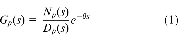
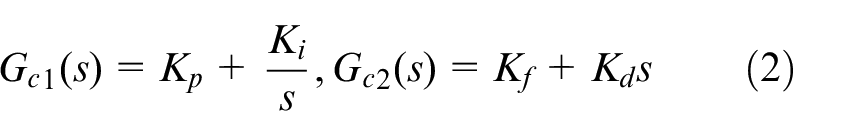
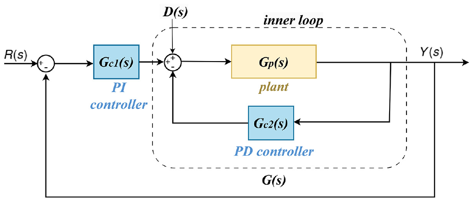
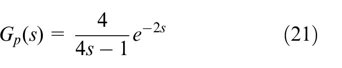
This section presents the SBL equations of the system with PI-PD controller, given in Figure 1. Gp(s) defines the time-delay system, Gc1(s) defines the PI controller and Gc2(s) defines the PD controller and are given in equations (1) and (2), respectively.
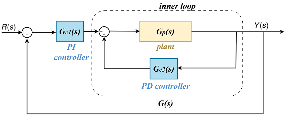
Block diagram of control system developed with PI-PD controller.
In equation (1), N p and D p represent the G p transfer function’s numerator and denominator polynomials, respectively. The main purpose here is to obtain the PI and PD controller parameters that make the closed-loop system stable. For this, the SBL analysis was carried out considering the studies in Onat, 18 Ozyetkin et al., 19 Ozyetkin and Toprak, 41 and Tan. 42
Obtaining SBL equations for PD control structure
In Figure 1, the characteristic equation for the inner loop, which includes a PD controller, can be expressible as in equation (3):
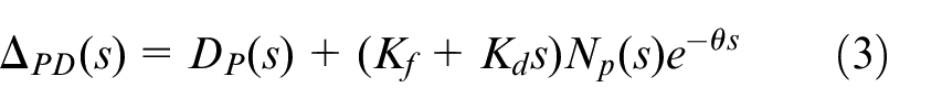
Since the SBL depends on the controller parameters and the frequency (ω), which can vary from 0 to infinity, the following equations are used to obtain the frequency range that makes the system stable and hence the set of controller parameters that make the system stable.
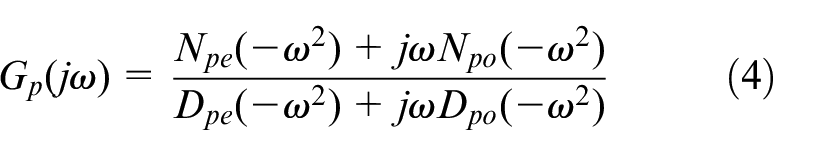
By typing s = jω in equation (1), Gp(jω) is obtained as in equation (4) and ΔPD(jω) in equation (5):
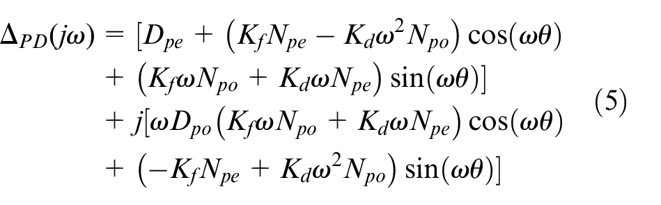
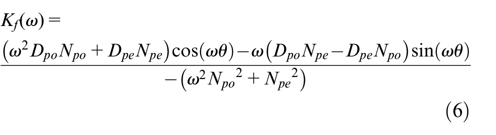
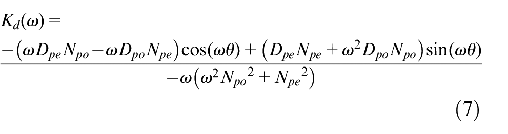
The equations Kf(ω) and Kd(ω) are obtained by setting the real parts and imaginary parts of ΔPD(jω) in equation (5) to 0, as shown in equations (6) and (7).
With the help of equations (6) and (7), SBL graph in the (K d , K f )-plane can be drawn as in Figure 2. However, there is a point to be noted here; if the denominator of equations (6) and (7) is equal to 0 at a certain frequency value, using this frequency will result in a discontinuous SBL and this will not interfere with the finding the controller values that make the system stable. Once the SBL is determined, it becomes essential to test whether there exist controller parameters that render the system stable. This is because, in cases where a RRB line and an infinite root boundary (IRB) line exist, they can partition the parameter plane into regions of stability and instability. The RRB line (Kf = Kf(0)) should be obtained by writing ω = 0 in equation (6). This occurs because a real root of ΔPD(s) in equation (3) has the potential to pass the imaginary axis at s = 0. When ω = 0, it is evident that the imaginary component of ΔPD(jω) as presented in equation (5) becomes zero. For the real part of equation (5) to be equal to zero, Kf must be equal to Kf(0). Therefore, the K f = Kf(0) determines the stability region boundary line. For a causal transfer function, the order of the denominator (D p ) must be greater than the numerator (N p ). In this case, a suitable transfer function is obtained and there is no infinite root boundary line. 42
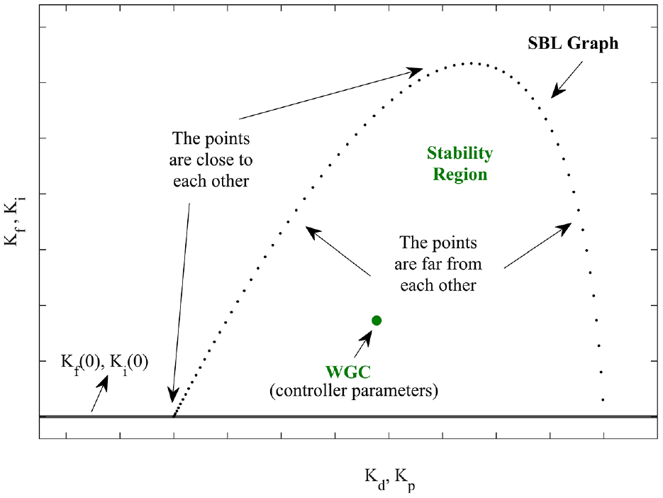
SBL graph for PI and PD controllers and implementation of WGC.
The SBL depends on the frequency (ω), which varies from 0 to infinity. As mentioned above, Kf(ω) = Kf(0) can be provided at a real ω greater than zero, since K f = Kf(0) is the boundary line of the SBL. If this positive real value of the frequency is called ωmax, drawing the SBL graph in between ω∈[0, ωmax] will be sufficient to obtain the (K d , K f ) parameters that provide stability. 42
Obtaining SBL equations for PI control structure
In the block diagram given in Figure 1, the inner loop closed-loop transfer function G(s), with PD controller, is expressed as in equation (8).
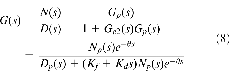
Taken as s = jω, G(s) can be expressed as follows.
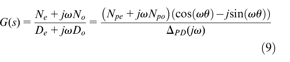
where,
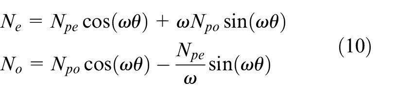
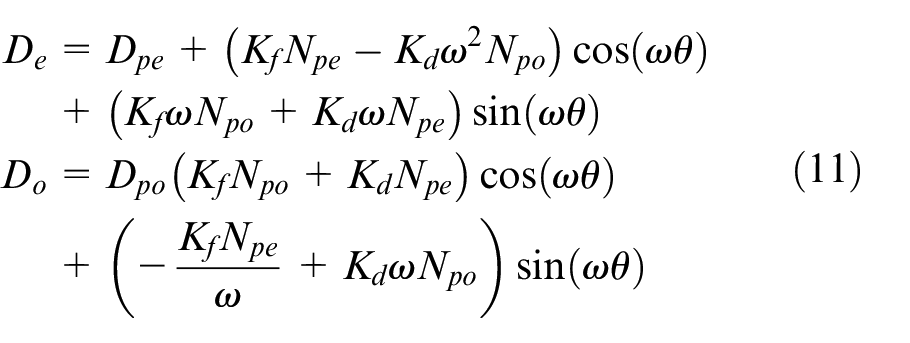
The method used to obtain the PI parameters is the same as in Section 2.1 and the equations are obtained as follows:
The outer loop closed loop characteristic equation is written as in equation (12):
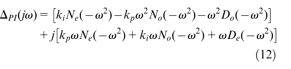
The equations Kp(ω) and Ki(ω) are obtained by setting the real and imaginary parts of ΔPI(jω) in equation (12) to 0, as shown in equations (13) and (14).
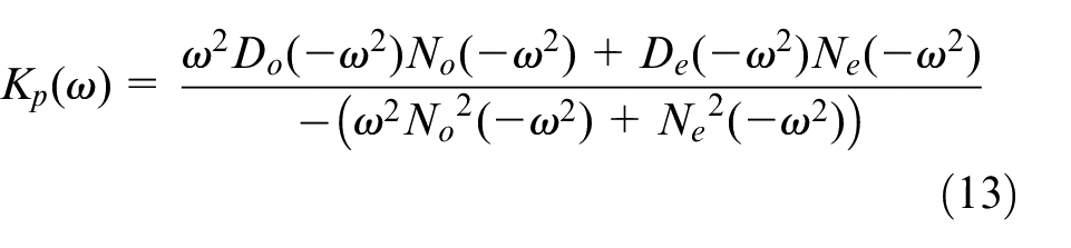

By solving equations (13) and (14), SBL in the (K p -K i ) plane is obtained as in Figure 2. The K p -K i parameter plane is separated into stability and instability regions by the SBL and K i = K i (0) = 0 line. 33 Because the real root of ΔPI(s) can cross the imaginary axis at s = 0, it can be concluded that IΔ = 0 and RΔ = 0, K i = 0, for ω = 0. 42
Stability region centroid methods
Within the SBL region, there are infinite combinations of controller parameters that stabilize the closed-loop system. However, any parameter combination within the SBL region can offer a better time response than any other parameter combination. Consequently, the identification of suitable points within the SBL region that satisfy desired performance criteria for controller parameters has been extensively researched in the literature. In this section, the WGC, CCSR and STM stability region centroid methods found in the literature are presented. In addition to these, as mentioned in the introduction, there are other methods available. However, these three methods constitute the basis of other methods. Therefore, the comparison of methods for PI-PD controller design has been made only for these three methods. These methods are introduced in the following subsections.
Weighted geometric center method
In Figure 2, the SBL graph obtained for the PD control structure is presented. This graph is generated by solving the equations K d (ω)–K f (ω) for each ω value in the range ω ∈ [0, ωmax] corresponding to the value ωmax satisfying Kf(ω) = Kf(0), as described in Section 2.1 and it is obtained by plotting it in the (K d , K f ) plane. This stability region consists of n (K d , K f ) coordinate points (K d1 , K f1 ), (K d2 , K f2 ),.., (K dn , K fn ). Since the K f (0) line is independent of ω and constitutes the boundary of the SBL, for K f (0) line, each (K d1 , K f1 ), (K d2 , K f2 ),.., (K dn , K fn ) pair is corresponding to ((K d1 , K f (0)), (K d2 , K f (0)),.., (K dn , K f (0)), respectively, as shown in Figure 2. These (K d , K f ) coordinates are at different locations for each ω; see Figure 2. When ω is small, the points are close, as ω increases, they are far and for very large ω values, they are too far. These points end at the RRB (K f = K f (0)). The n results obtained here are related to the step size (Δ ω ) of ω. Decreasing the step interval will increase the number of samples and will ensure that the result obtained from the controller calculation methods will be more accurate.
The WGC method introduced by Onat 37 provides to get the appropriate operating point in the stability region with the help of all the coordinate points obtained depending on the ω on the SBL for the controller parameters. Accordingly, for the SBL graph in Figure 2, the PD controller values in equation (15) are calculated:
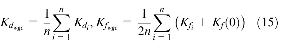
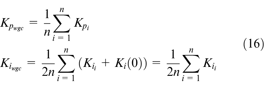
The PI controller SBL graph, as in Figure 2, is generated by resolving the equations K p (ω)–K i (ω) for each ω value in the range ω ∈ [0:Δω:ωmax] corresponding to the value ωmax satisfying Ki(ω) = Ki(0) = 0 similar to the PD one and it is obtained by plotting it in the (K p , K i ) plane. Accordingly, the PI controller values are calculated as in equation (16):
Convex stability region method
The method introduced in Onat 18 is an analytical method calculated with the help of SBL graph and is named CCSR. According to the method, the stable region obtained by the combination of the peak and corner points on the SBL as in Figure 3 defines the CSR.
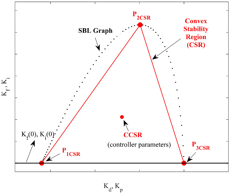
SBL graph for PI and PD controllers and implementation of CSR.
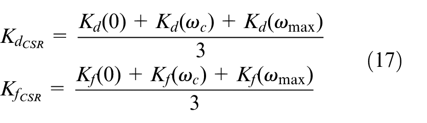
The coordinates of the vertex and vertices of the SBL graph in the (K d , K f ) plane obtained for the PD controller are expressed as P1(Kd(0), Kf(0)), P2(Kd(ωc), Kf(ωc)) and P3(Kd(ωmax), Kf(ωmax)). Here P1 denotes the corner point corresponding to ω = 0. If the frequency point where Kf reaches its maximum value is Kf(ωc) = Kfmax, then the corresponding Kd value at this frequency is calculated as Kd(ωc). This point is referred to as the P2 corner. P3 represents the corner point where the SBL region corresponds to ω = ωmax. Accordingly, the PD controller parameters are calculated with the help of points P1, P2, and P3 as in equation (17):
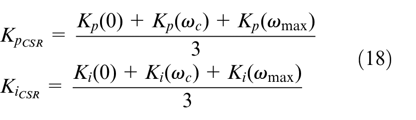
Similarly, by finding the P1, P2, and P3 points for the PI controller, the controller parameters are calculated as in equation (18):
Stability triangle method
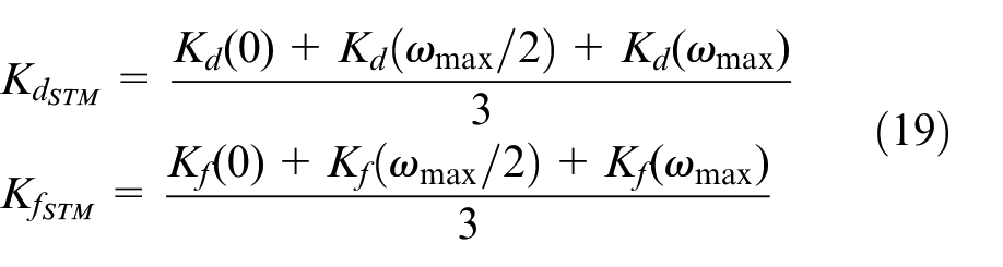
Similar to the method introduced in Onat 18 , an analytical controller design formulas called STM are given for PI controller by Yuce. 44 The method is based on SBL as the WGC and CSR methods, see Figure 4. The method was applied for the first time in this study for PI-PD control integrating and resonance with time delay systems and the controller formulas were obtained in equations (19) and (20). In STM, unlike CSR, point P2 is expressed as the corner point corresponding to ω = ωmax/2, that is, P2(Kd(ωmax/2), Kf(ωmax/2)) and PD controller parameters are calculated as in Equation (19) with the help of points P1, P2, and P3:
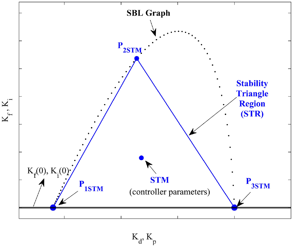
SBL graph for PI and PD controllers and implementation of STM.
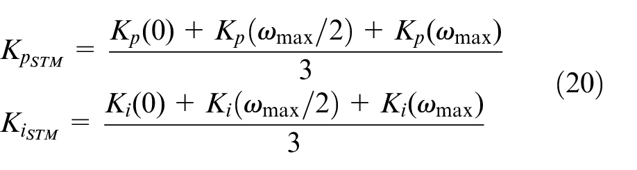
By finding the P1, P2, and P3 points for the PI controller, the controller parameters are calculated as in equation (20):
Simulation studies
In this section, four different examples are discussed. These examples are implemented in the block diagram in Figure 5 with the methods described in Section 2. UFOPTD, unstable second order plus time delay (USOPTD), resonant SOPTD (R-SOPTD), integrating SOPTD (IU-SOPTD) models are examined, respectively. A unit step signal is applied to the input signal (R(s)) and the step responses are obtained accordingly. In order to examine the disturbance rejection performance of the systems, the disturbance signal (D(s)) was applied and accordingly the servo response (
Block diagram of the closed loop control system designed with the PI-PD controller used in the simulation study.
Firstly, the SBL for the PD structure in the inner loop is plotted in K d -K f plane as given in Figure 6. Then, WGC, CCSR and STM points were determined within this stability region as illustrated in Figure 6. Here, using equation (6), it is obtained to be Kf(0) = 0.25. The positive frequency value that makes equation (6) equal to the 0.25 is ωmax = 1.3932. Therefore, the SBL for K d -K f plane is drawn as showed in Figure 6 for the range of ω = [0:0.01:1.3932]. K d -K f controller parameter pairs obtained from each method for the PD from inner loop given in Figure 6 are used one by one for calculating PI in the outer loop. In this case, by using the PI controller within outer loop, the critical frequency value that makes equation (14) equal to 0 should be determined to plot the K p -K i SBLs for each K d -K f pair. For this example, by using K d -K f pairs at WGC, STM and CCSR points in Figure 6, the critical frequency values (ωmax) for each method are 0.7127, 0.7273, and 0.8 rad/s, respectively. As a result, K p -K i SBLs for each method were plotted as in Figure 7 with ω = [0:0.01:ωmax]. WGC, STM, and CCSR points were determined under the PI SBL’s of each method. Therefore, closed loop transfer functions were obtained using the structure in Figure 5 with K d , K f , K p , K i values obtained from each method. Thus, the servo and regulatory responses of the model are examined for each method. Besides, the system responses are examined in the case of a change in model parameters to analyze the robustness of the methods.
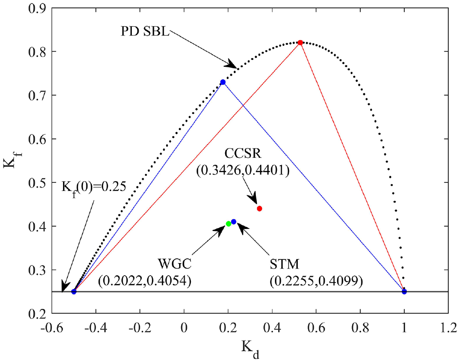
SBL for PD control and application of WGC-CSR-STM for example 1.
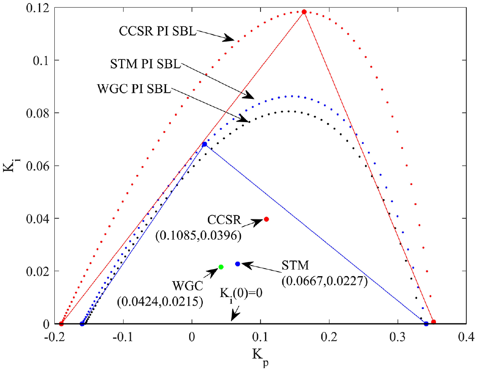
SBLs obtained in each method for PI control and application of WGC-CSR-STM for example 1.
Figure 8 shows the servo and regulatory responses according to K f , K d , K p , K i values obtained using each method. For the servo response, a reference signal with amplitude R = 1 is added the system at t = 0 whereas for the regulatory response a disturbance signal with an amplitude of D = 0.5 is added to the controlled system at t = 30 s. Figure 9 shows the time domain performance metrics for the servo response of each method in the form of a bar graph.
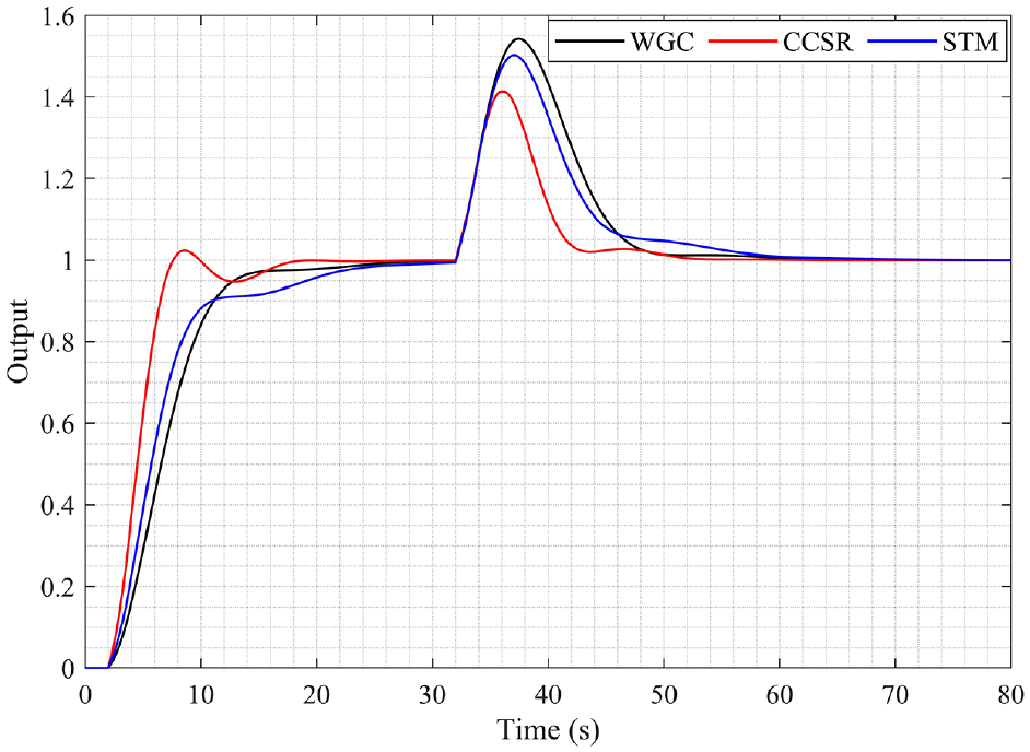
Servo and regulatory responses of the nominal system according to the K f , K d , K p , K i values obtained by each method for example 1.
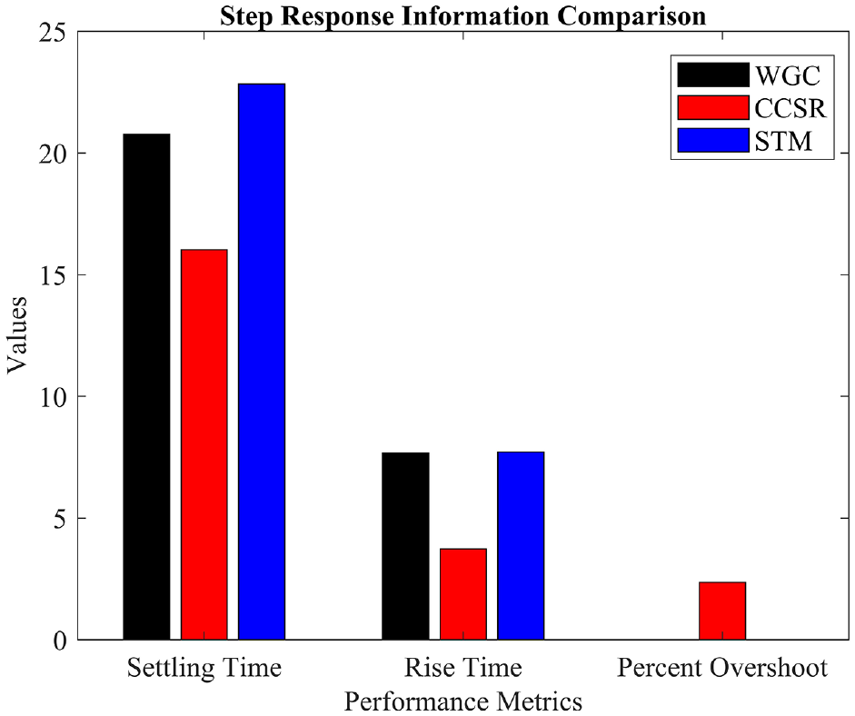
Time domain performance metrics for the servo response of the nominal system according to the K f , K d , K p , K i values obtained by each method for example 1.
For the WGC, CCSR, and STM methods, the rise times were 7.667, 3.73, and 7.73 s respectively; the settling times were 20.84, 16.0, and 22.92 s respectively and maximum overshoots were obtained as 0%, 2.36%, and 0% respectively. Accordingly, the CCSR method has the lowest settling time and rise time values; this inference is based on the analysis of Figure 8 that shows servo and regulatory responses and Figure 9 that shows the time domain performance metrics. On the other hand, while a certain amount of overshoot is observed in the CCSR method, a non-overshoot response is obtained in the WGC and STM methods. When a disturbance of 0.5 amplitude is added to the nominal system at t = 30 s, all methods successfully reject the disturbance as shown in Figure 8. In terms of disturbance rejection, the CCSR method performed a faster response with lower overshoot than the other methods. In addition, the system parameters given in equation (21) have been changed by ±10% to examine the robustness analysis of the system. Accordingly, equations (22) and (23) give the transfer functions of the nominal parameters of the system perturbed by +10% and −10%, respectively.
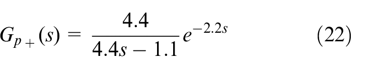
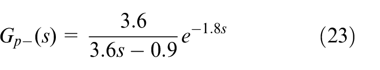
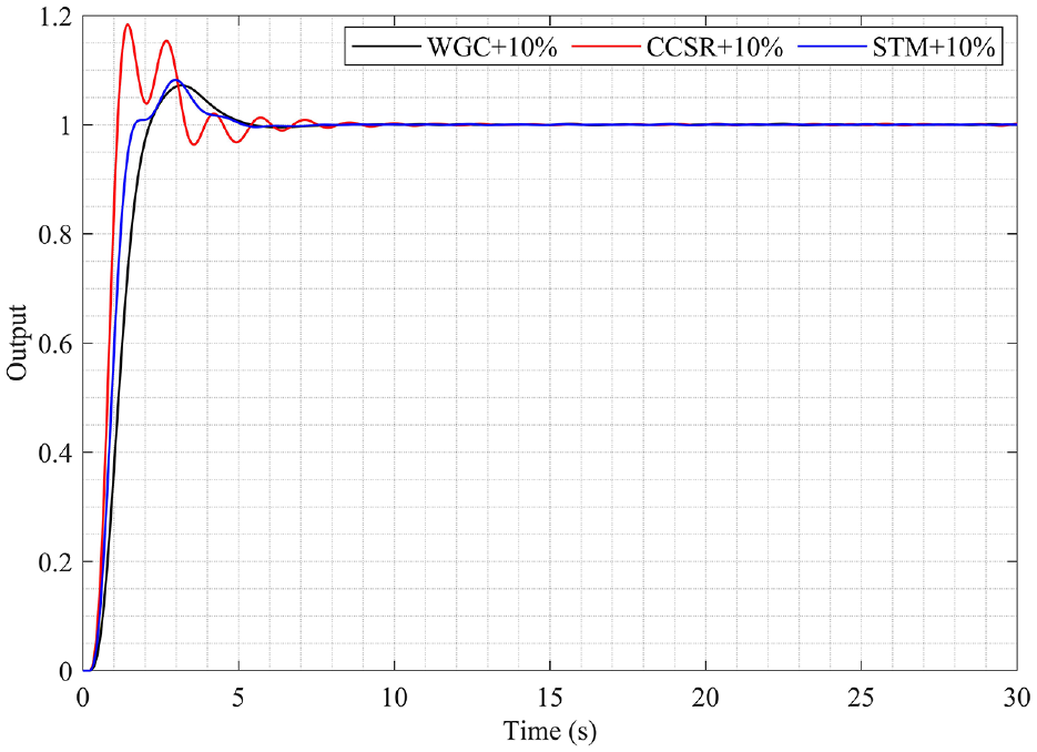
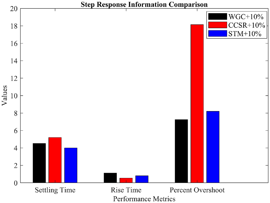
Figure 10 illustrates the step response of the system perturbed by +10% as described in equation (22), with the K f , K d , K p , and K i values determined for the nominal system using each of the methods explained. Accordingly, the bar graph of the time domain performance metrics obtained from servo response of each method is given in Figure 11.
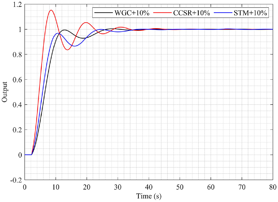
Step responses of +10% perturbed system according to K f , K d , K p , K i values obtained for the nominal system using each method for example 1.
Time domain performance metrics for step response of +10% perturbed system based on K f , K d , K p , K i values obtained for the nominal system using each method for example 1.
When examining Figure 10, which the servo responses of the perturbed by 10% and Figure 11, which time domain performance metrics for the servo response, for the WGC, CCSR, and STM methods the rise times were 6.24, 3.25, and 5.41 s, respectively; the settling times were 0.90, 0.84, and 0.87 s, respectively and maximum overshoots were obtained as 0.52%, 15.09%, and 0.13%, respectively. Accordingly, the CCSR method has the lowest settling time and rise time values. It is seen that the WGC, CCSR, and STM methods have the lowest settling time, respectively. On the other hand, while the highest overshoot is observed in the CCSR method, a lower overshoot is obtained in the WGC and STM methods.
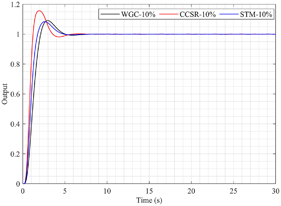
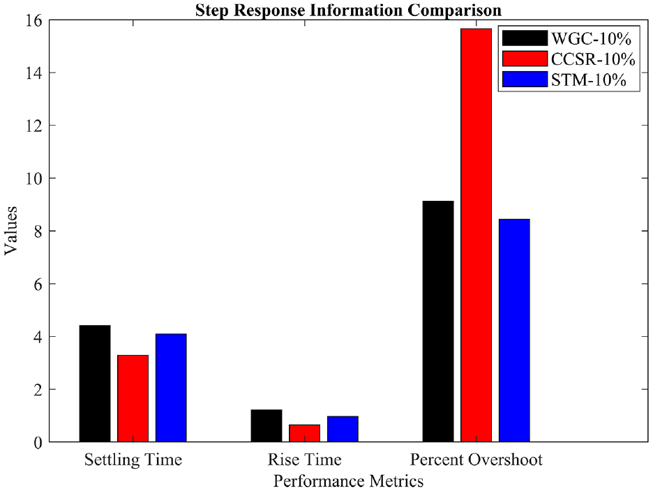
Figure 12 shows the servo response of the −10% perturbed system in equation (23) according to the K f , K d , K p , K i values obtained for the nominal system using each method. Accordingly, the bar graph of the time domain performance metrics of the servo response of each method is given in Figure 13.
Step responses of −10% perturbed system according to K f , K d , K p , K i values obtained for the nominal system using each method for example 1.
Time domain performance metrics for step response of −10% perturbed system based on K f , K d , K p , K i values obtained for the nominal system using each method for example 1.
When the servo responses of the system parameters perturbed by −10% in Figure 12 and the time domain performance metrics shown in Figure 13 are analyzed, for the WGC, CCSR, and STM methods, the rise times were 8.97, 4.96, and 9.67 s respectively; the settling times were 15.88, 11.17, and 21.33 s respectively and maximum overshoots were obtained as 0.40%, 0%, and 0.06% respectively. The methods with the lowest settling time and rise time is seen from CCSR, WGC, and STM methods, respectively. On the other hand, no overshoot response is obtained from the CCSR method, while a very low overshoot is obtained from the WGC and STM methods.
These results of the analysis show that PI-PD controllers with these stability region centroid approaches for a UFOPTD system may provide a suitable servo and regulatory response. When the reference tracking (servo) and disturbance rejection (regulatory) performances of the methods are compared, it is seen that no method is superior to the others in terms of all performance criteria. In addition, in the case of the robustness analysis, all approaches exhibit successful step response performance and retain their stable condition despite changes in system characteristics. When the overall system performance is evaluated, it is evident that the methods applied to perturbed models exhibit specific advantages and disadvantages concerning specified performance metrics, as in the nominal system.
First, Kf(0) = 1 is obtained using equation (6). The positive frequency value that makes equation (6) equal to 1 is ωmax = 5.48 rad/s. Therefore, the SBL graph for the (K d -K f )-plane was drawn within the between of ω = [0:0.01:5.48]. The SBL for the inner loop containing the PD controller and the point of the K d -K f controller parameter pairs obtained from each method can be seen in Figure 14. The K d -K f pairs obtained from each method are substituted in equation (8) and used to calculate the PI parameters in the outer loop. When the K d -K f pair from each method is used, different critical frequency values (ωmax) are formed, which makes equation (14) zero. These critical frequency values were calculated as 2.9423, 3.1221, and 3.4552 rad/s for WGC, STM, and CCSR, respectively. Therefore, the SBL for the K p -K i plane was drawn for ω = [0:0.01:ωmax] using each method critical frequency and can be seen in Figure 15. The SBL for the PI outer loop and the point of the K p -K i controller parameter pairs obtained from each method can be seen in Figure 15. As a result, closed-loop transfer functions were obtained by using the K f , K d , K p , K i values obtained from each method.
SBL obtained for PD control and application of WGC-CSR-STM for example 2.
SBLs obtained in each method for PI control and application of WGC-CSR-STM for example 2.
Figure 16 shows the servo and regulatory responses based on the values of K f , K d , K p , and K i obtained through each stability region centroid methods. For the servo response, a reference signal with amplitude 1 is added the system at t = 0 s whereas for the regulatory response a disturbance signal with an amplitude of D = 0.5 is added to the control system at t = 16 s. Figure 17 presents time-domain performance metrics for the servo response of each method and depicted in the form of a bar graph.
Servo and regulatory responses of the nominal system according to the K f , K d , K p , K i values obtained by each method for example 2.
Time domain performance metrics for the servo response of the nominal system according to the K f , K d , K p , K i values obtained by each method for example 2.
For the WGC, CCSR, and STM methods, the rise times were 1.66, 0.80, and 1.29 s respectively; the settling times were 5.27, 4.28, and 4.56 s respectively and maximum overshoots were obtained as 3.89%, 10.38%, and 2.42% respectively. As a result, when examining the servo and regulatory responses in Figure 16 and the time domain performance metrics in Figure 17, it is observed that the methods with the lowest settling time and rise time are CCSR, STM, and WGC respectively. In contrast, while a significant overshoot is observed from the CCSR method, both the WGC and STM methods have yielded responses with comparatively lower levels of overshoot than that of CCSR. As depicted in Figure 16, when a disturbance of amplitude D = 0.5 is introduced to the nominal system at t = 16 s, all methods effectively reject the disturbance. Here, in terms of disturbance rejection, the CCSR method has exhibited superior performance compared to other methods, with a faster response and lower levels of overshoot.
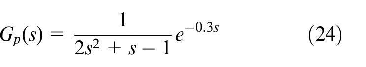
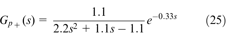
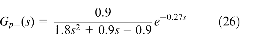
Furthermore, to examine robustness analysis, the system parameters given in equation (24) have been changed by ±10%. Accordingly, equations (25) and (26) present the perturbed transfer functions of this system, corresponding to +10% and −10% variations, respectively.
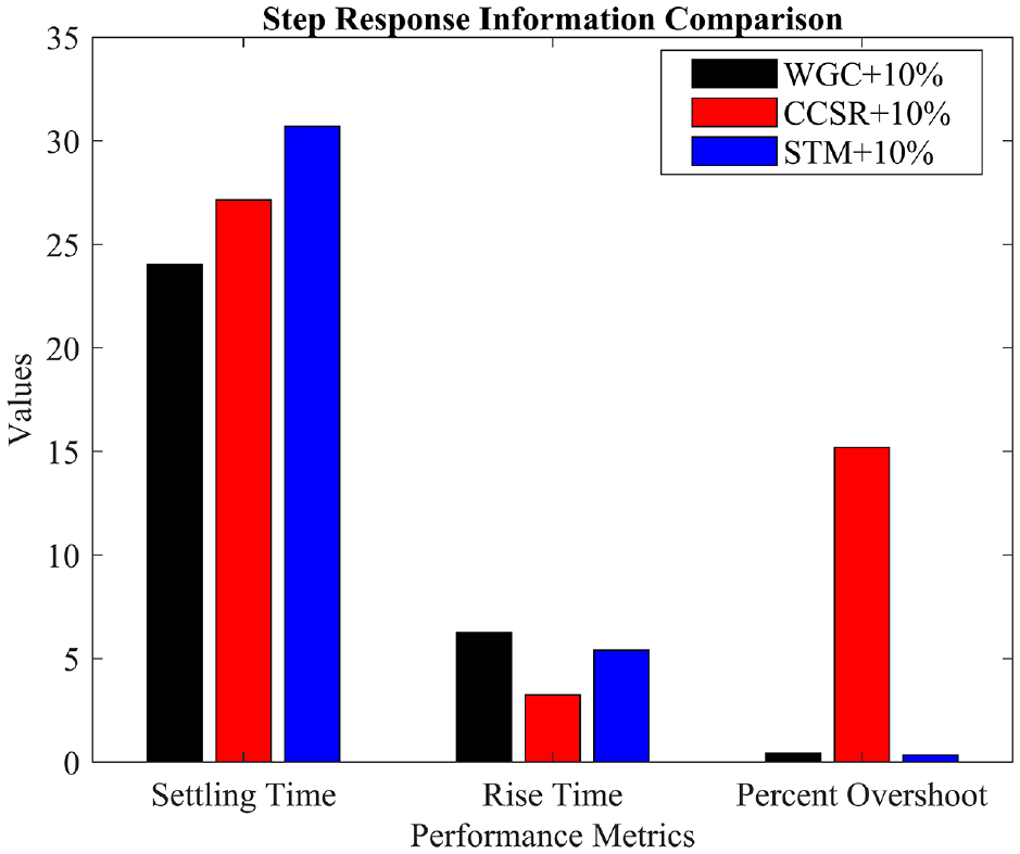
In Figure 18, the servo responses of the perturbed system, with a +10% variation as given in equation (25), is presented based on the K f , K d , K p , and K i values obtained for the case of the nominal system using each stability region centroid method. Subsequently, Figure 19 illustrates a bar graph depicting the time domain performance metrics for the servo response of each method.
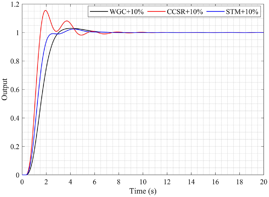
Step responses of +10% perturbed system according to K f , K d , K p , K i values obtained for the nominal system using each method for example 2.
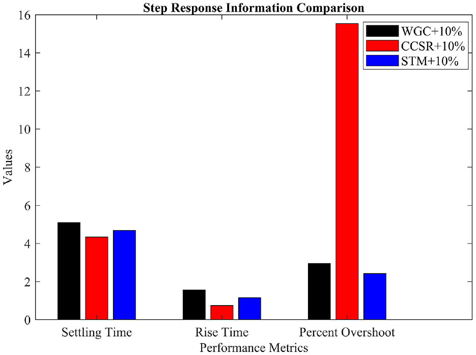
Time domain performance metrics for step response of +10% perturbed system based on K f , K d , K p , K i values obtained for the nominal system using each method for example 2.
When analyzing Figure 18, which illustrates the servo responses of the perturbed system for the WGC, CCSR and STM methods under +10% variation, along with the time-domain performance metrics shown in Figure 19, the rise times are obtained 1.56, 0.74, and 1.15 s, respectively, the settling times are obtained 5.10, 4.35, and 4.68 s, respectively. Maximum overshoots were obtained as 2.96%, 15.63%, and 2.44%, respectively. These results show that the methods yielding the most favorable settling time and rise time outcomes follow the sequence of CCSR, STM and WGC. It should be noted, however, that the CCSR method exhibits an extremely high overshoot, whereas both the WGC and STM methods exhibit a lower overshoot.
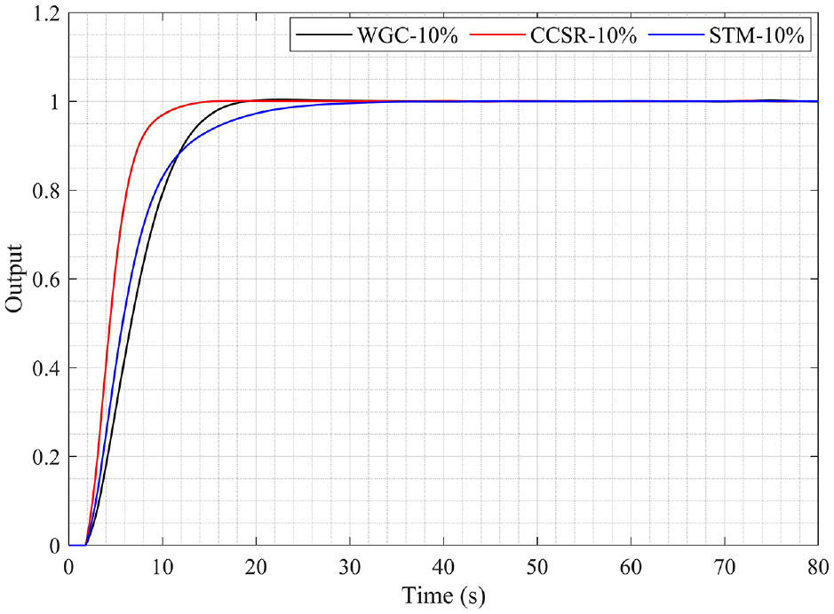
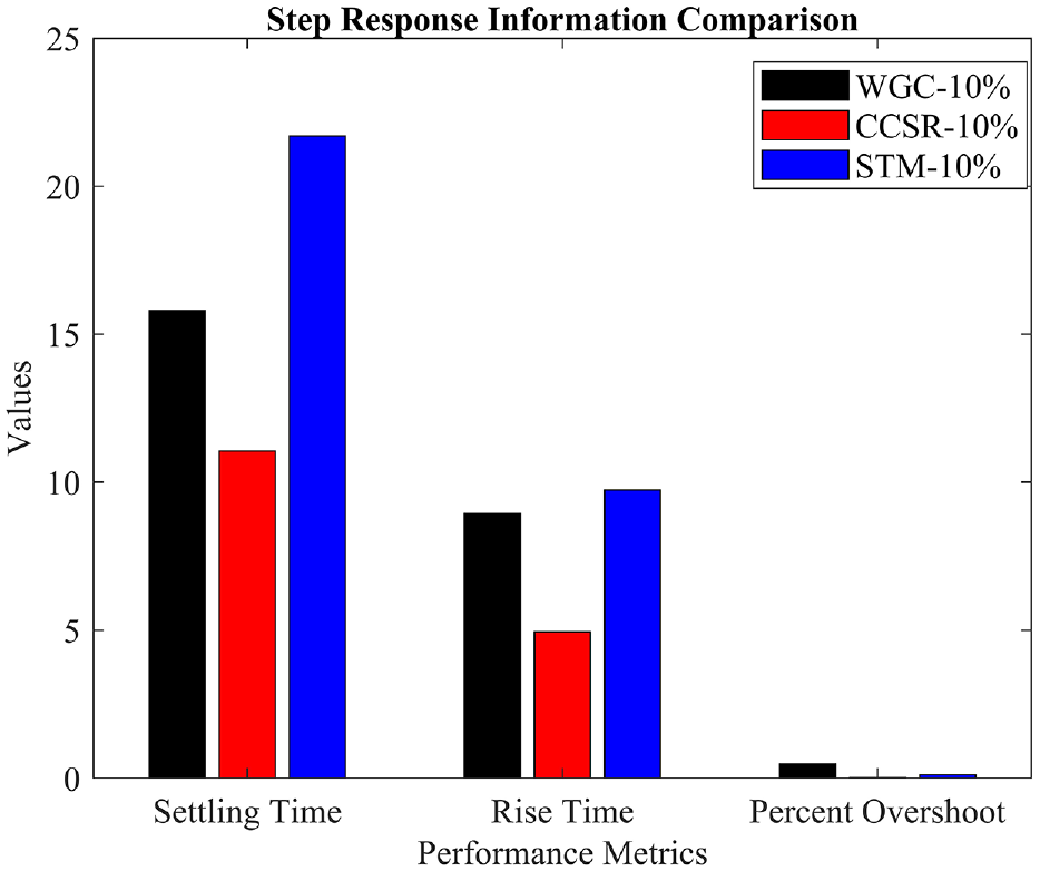
In Figure 20, the perturbed system’s step response with a −10% variation as given in equation (26), based on the K f , K d , K p , and K i values obtained for the nominal system using each stability centroid method, is presented. Consequently, Figure 21 depicts a bar graph illustrating the time domain performance metrics for the servo response of each method.
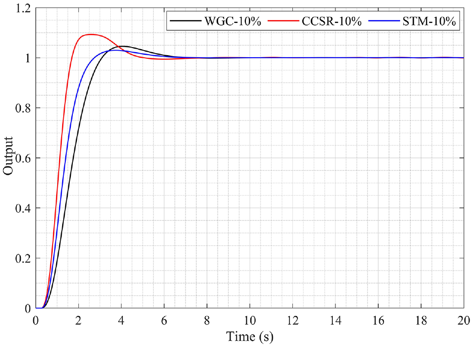
Step responses of −10% perturbed system according to K f , K d , K p , K i values obtained for the nominal system using each method for example 2.
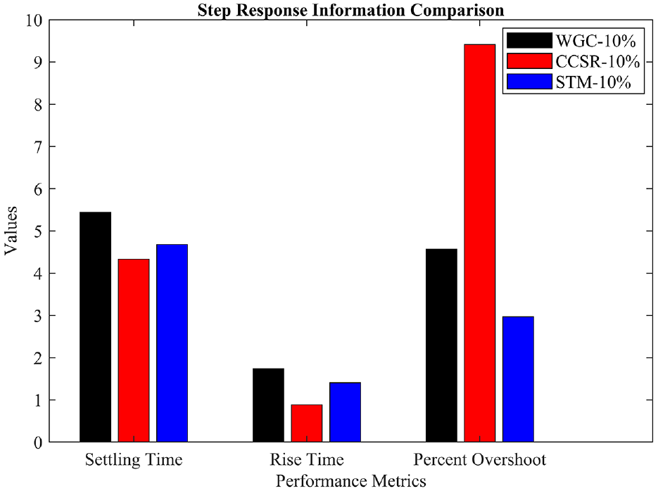
Time domain performance metrics for step response of −10% perturbed system based on K f , K d , K p , K i values obtained for the nominal system using each method for example 2.
Based on analyzing the time domain performance metric for the servo response for the WGC, CCSR, and STM methods, the rise times are obtained 1.74, 0.89, and 1.41 s, respectively. The settling times are 5.44, 4.30, and 4.67 s, respectively. Accordingly, it becomes evident that the methods with the lowest settling time and rise time are the CCSR, STM, and WGC, respectively. However, it is worth noting that the CCSR method exhibits a significantly higher overshoot, 9.39%, whereas the WGC and STM methods achieve relatively lower levels of overshoot, 4.56% and 2.96%, respectively.
Based on these analyses, it can be observed that when utilizing these stability region centroid methods, PI-PD controllers yield favorable servo and regulatory responses for a USOPTD system. When assessing the methods’ abilities for reference tracking (servo) and disturbance rejection (regulatory), it has been realized that no single method consistently outperforms the others for all performance metrics. Furthermore, concerning robustness analysis, all methods have maintained stability and achieved successful step responses despite variations in system parameters. Upon considering the overall system performance, it is evident that, like the nominal system, the methods exhibit advantages and disadvantages only in specific performance criteria for the perturbed system as well.
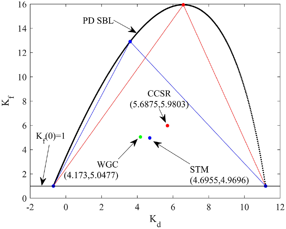
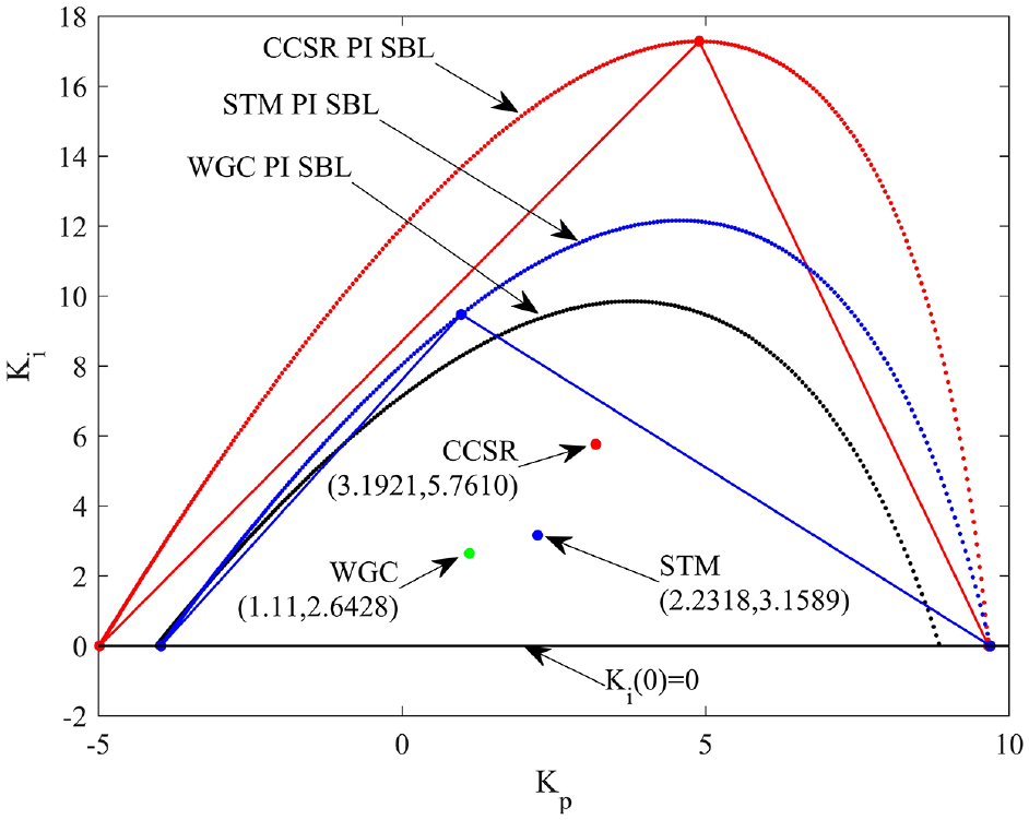
Kf(0) = −1 was obtained using equation (6) to obtain the SBL of the PD structure in the inner loop. The positive frequency value that equates equation (6) to −1 was determined as ωmax = 15.7611 rad/s. Therefore, the SBL as a function of K d -K f has been plotted in the range of ω = [0:0.01: 15.7611]. The results obtained are shown in Figure 22. Figure 22 shows the pairs of K d -K f controller parameters obtained from each method for the inner loop containing the PD controller. The K d -K f pairs obtained from each method are substituted into equation (8) and used to calculate the PI controller K p -K i parameters in the outer loop. When utilizing the K d -K f pairs obtained from each method, varying critical frequency values (ωmax) emerge that equates equation (14) to zero. These values were calculated to be 8.5106, 10.0126, and 9.0517 rad/s for WGC, STM, and CCSR, respectively Therefore, the SBL for the K p -K i plane was drawn for ω = [0:0.01: ωmax] using each method critical frequency and can be seen in Figure 23. The SBL for the PI outer loop and the point of the K p -K i controller parameter pairs obtained from each method can be seen in Figure 23. As a result, closed-loop transfer functions were obtained using the structure in Figure 5 for the K f , K d , K p , and K i values obtained by each method.
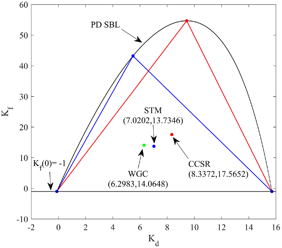
SBL obtained for PD control and application of WGC-CSR-STM for example 3.
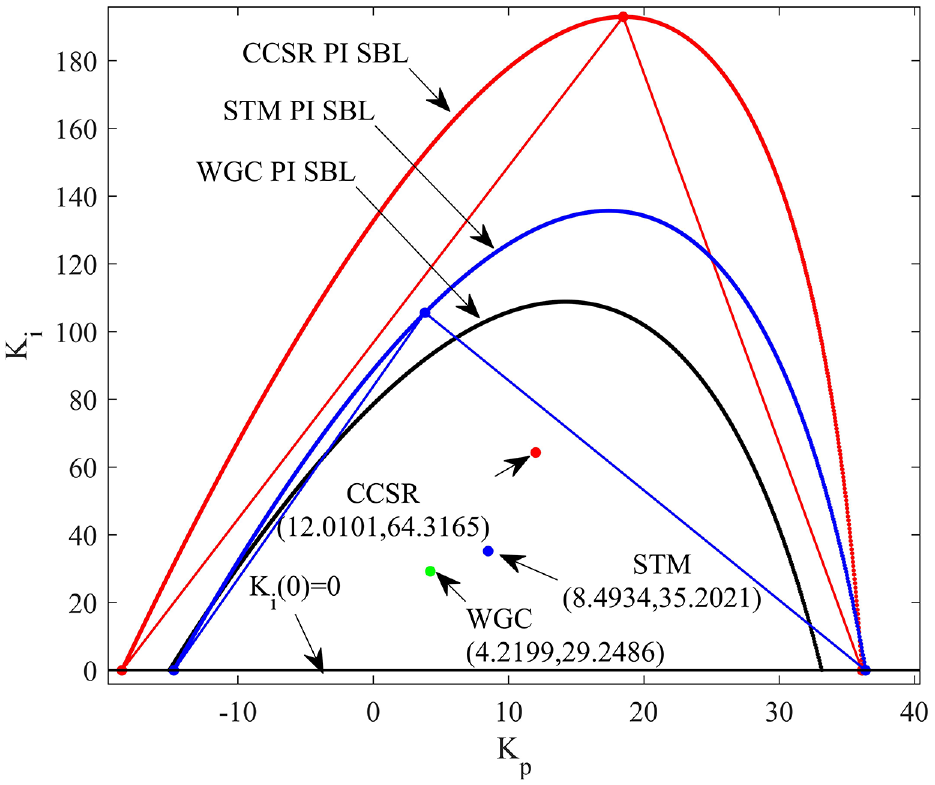
SBLs obtained in each method for PI control and application of WGC-CSR-STM for example 3.
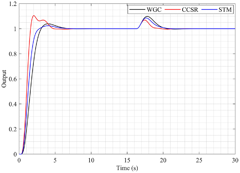
In the Figure 24, the servo and regulatory responses are provided based on the K f , K d , K p , and K i values obtained using each stability region centroid method. For the servo response, a reference signal with amplitude 1 is added the system at t = 0 s whereas for the regulatory response a disturbance signal of amplitude D = 1 is added to the PI-PD controlled system at t = 5 s. In Figure 25, a bar graph has been presented depicting the time domain performance metrics for the servo response of each method.
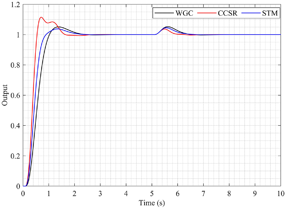
Servo and regulatory responses of the nominal system according to the K f , K d , K p , K i values obtained by each method for example 3.
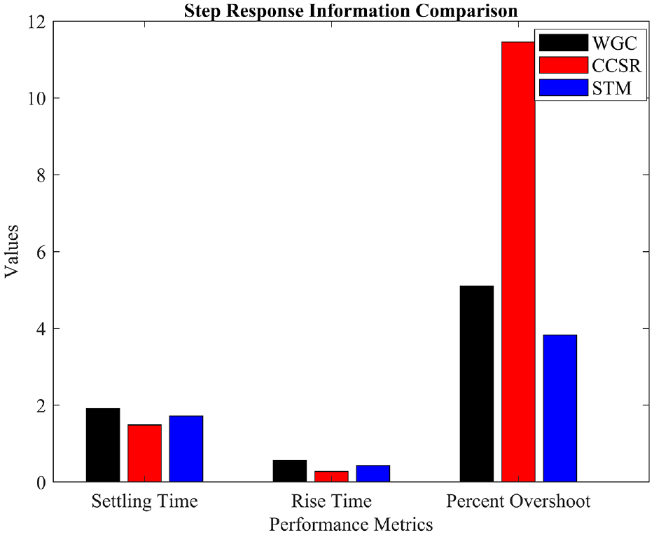
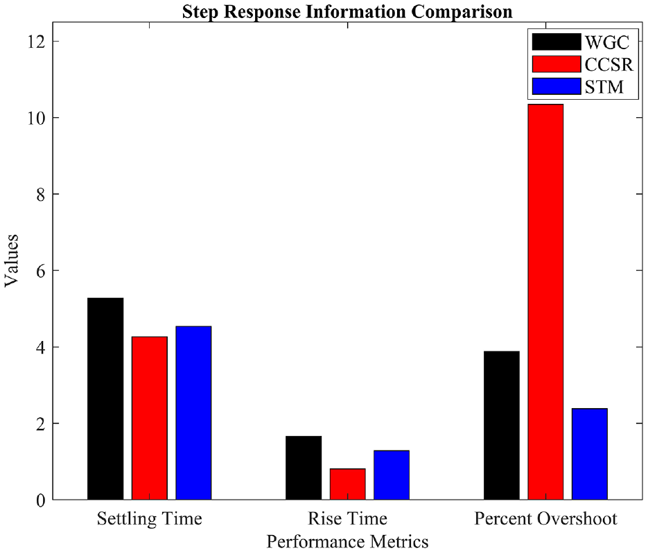
Time domain performance metrics for the servo response of the nominal system according to the K f , K d , K p , K i values obtained by each method for example 3.
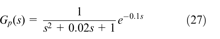
As a result, when examining the servo and regulator responses presented in Figure 24 along with the time-domain performance metrics shown in Figure 25, it is evident that the settling times obtained from the CCSR, STM, and WGC methods are 1.48, 1.73, and 1.92 s respectively. Therefore, it is easefully seen that the CCSR method has the lowest settling time among them. Similarly, the rise times were obtained as 0.28, 0.44, and 0.56 s for the CCSR, STM, and WGC methods, respectively and the CCSR appears as the method with the lowest rise time. On the other hand, while a high overshoot is observed from the CCSR method, 11.35%, a relatively lower overshoot response is obtained from the WGC and STM methods, 5.09% and 3.87%, compared to CCSR. When a disturbance of D = 1 is included to the system at t = 5 s, all methods successfully reject the disturbance as shown in Figure 24. In terms of disturbance rejection, the CCSR method performed with less overshoot and faster response than the other methods. Additionally, to conduct a robustness analysis of the system, the system parameters given in equation (27) are changed by ±20%. Accordingly, the transfer functions of the system perturbed by +20% and −20% are given in equations (28) and (29), respectively.
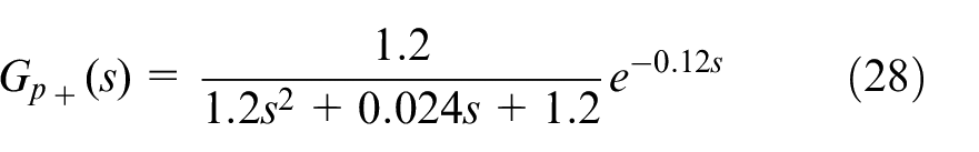
Figure 26 shows the servo responses of the + 20% perturbed system in equation (28) according to the K f , K d , K p , and K i values obtained for the nominal system using each method. Accordingly, the bar graph of the time-domain performance metrics for the servo response of each method is given in Figure 27.
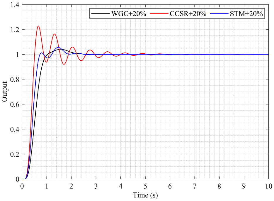
Step responses of +20% perturbed system according to K f , K d , K p , K i values obtained for the nominal system using each method for example 3.
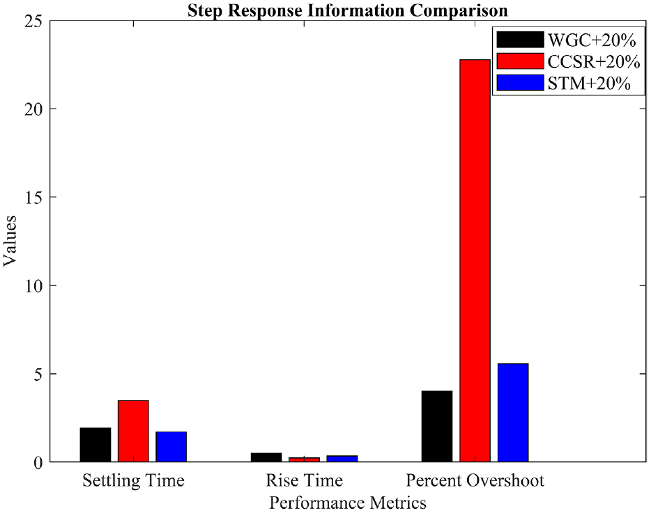
Time domain performance metrics for step response of +20% perturbed system based on K f , K d , K p , K i values obtained for the nominal system using each method for example 3.
Upon analyzing Figures 26 and 27, it is evident that the methods with the lowest settling time are the STM, WGC and CCSR methods, 1.71, 1.95, and 3.18 s, respectively. For the lowest rise time, the sequence is the CCSR, STM and WGC methods, 0.24, 0.36, and 0.50 s. However, it’s important to note that while the CCSR method demonstrates a significant overshoot as 22.74%, the WGC and STM methods achieve a relatively lower level of overshoot as 4.17% and 5.54%.
Figure 28 shows the step responses of the −20% perturbed system in equation (29) according to the K f , K d , K p , K i values obtained for the nominal system using each method. Accordingly, the time domain performance metrics bar graph for the servo response of each method is given in Figure 29.
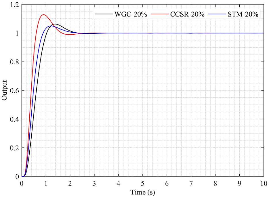
Step responses of −20% perturbed system according to K f , K d , K p , K i values obtained for the nominal system using each method for example 3.
Time domain performance metrics for step response of −20% perturbed system based on K f , K d , K p , K i values obtained for the nominal system using each method for example 3.
When examining Figure 28, the servo responses of the perturbed system with a −20% variation and time domain performance metrics for the servo response depicted in Figure 29, it is observed that the methods with the lowest settling time and rise time are, in sequence, CCSR, STM, and WGC methods. Here, the settling times are 1.49, 1.73, and 1.93 s and the rise times are 0.33, 0.50, and 0.60 s for the CCSR, STM, and WGC methods, respectively. On the other hand, it’s important to note that the CCSR method shows a significantly high overshoot, 12.83%, whereas the WGC and STM methods achieve a comparatively lower overshoot as 6.24% and 4.94%, than that of CCSR.
Based on these analyses, it is evident that when employing these stability region centroid methods, PI-PD controllers yield favorable servo and regulatory responses for an RSOPTD system. Upon examining the methods’ performance in reference tracking and disturbance rejection, it has been determined that no single method exhibits superior performance across all performance criteria. Additionally, through robustness analysis, all methods have maintained stability and achieved successful step responses despite variations in system parameters. From a system performance perspective, it can be concluded that, as in the nominal system, when dealing with a perturbed system, the methods present advantages and disadvantages in the specific performance criteria.
To obtain the SBL of the PD structure in the inner loop, Kf(0) = 0 was determined using equation (6). The positive frequency value that makes equation (6) = 0 is ωmax = 7.1602 rad/s. Therefore, the SBL depending on K d -K f was plotted in the range of the ω = [0:0.01: 7.1602]. The obtained results are given in Figure 30. Figure 30 shows the pairs of K d -K f controller parameters obtained from each method for the PD inner loop. Here, the K d -K f pairs obtained from each method are substituted in equation (8) and used to calculate the PI controller K p -K i parameters in the outer loop. When utilizing the K d -K f pairs obtained from each method, distinct critical frequency values (ωmax) are emerged that equates equation (14) to zero. These values were calculated as 3.9046, 4.6267, and 4.1853 rad/s for WGC, STM and CCSR, respectively. As a result, with the help of these ω = [0:0.01: ωmax] values, K p -K i plane PI SBLs were plotted for each method using PI structure in the outer loop, as shown in Figure 31. As a result, the K f , K d , K p , and K i values obtained using each method have been utilized to formed closed-loop transfer functions using the structure depicted in Figure 5.
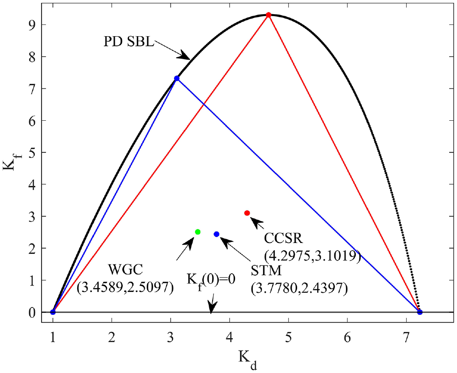
SBL for PD control and application of WGC-CSR-STM for example 4.
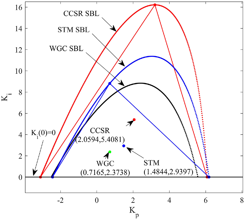
SBLs obtained in each method for PI control and application of WGC-CSR-STM for example 4.
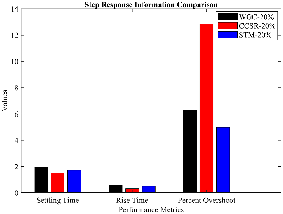
Figure 32 shows the servo and regulatory responses obtained according to K f , K d , K p , and K i values obtained using each method. For the servo response, a reference signal with amplitude 1 is added the system at t = 0 s whereas for the regulatory response a disturbance signal with an amplitude of D = 0.5 is included to the control system at t = 15 s. Figure 33 shows the time domain performance measures for the servo response of each method in the form of a column graph.
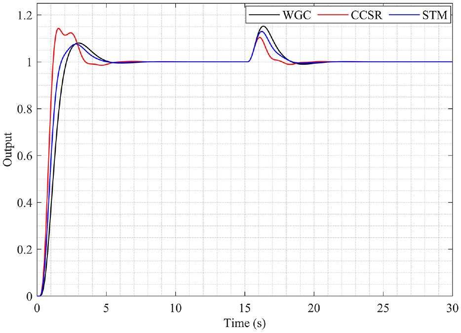
Servo and regulatory responses of the nominal system according to the K f , K d , K p , K i values obtained by each method for example 4.
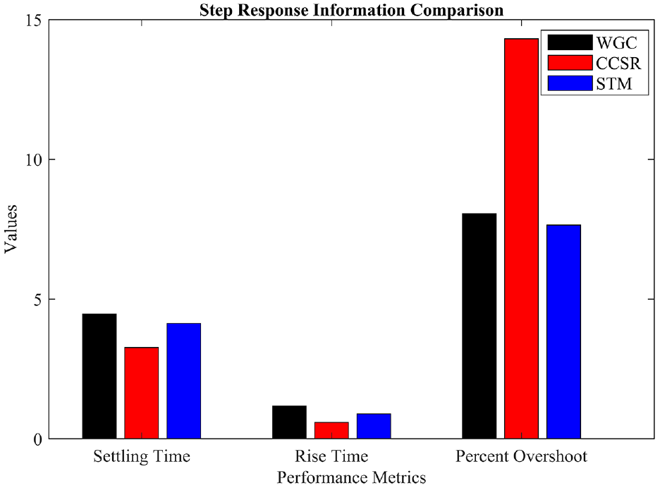
Time domain performance metrics for the servo response of the nominal system according to the K f , K d , K p , K i values obtained by each method for example 4.
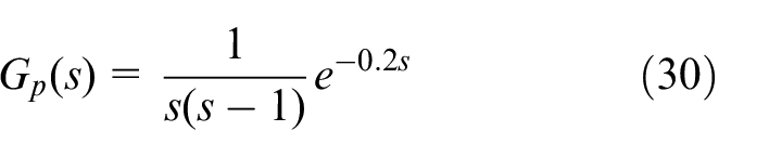
Accordingly, when the servo and regulatory responses in Figure 32 and the time domain performance metrics of the servo response in Figure 33 are analyzed, the methods with the lowest settling time and rise time are the CCSR, STM, and WGC, respectively. The settling times are 3.26, 4.11, and 4.72 s and the rise times are 0.60, 0.90, and 1.18 s, respectively for the CCSR, STM, and WGC. On the other hand, while an extremely high overshoot as 14.22% is observed from the CCSR method, a relatively lower overshoot response, as 8.05% and 7.59%, is obtained from the WGC and STM methods compared to CCSR. When a disturbance of D = 0.5 is added to the controlled system at t = 15 s, all methods successfully reject the disturbance, as shown in Figure 32. Here, in terms of disturbance rejection, the CCSR method performed with a lower overshoot in a shorter time than the other methods. Furthermore, the system parameters provided in equation (30) were altered by ±10% to assess the robustness of the system. Accordingly, the transfer functions of the system perturbed by +10% and −10% are given in equations (31) and (32), respectively.
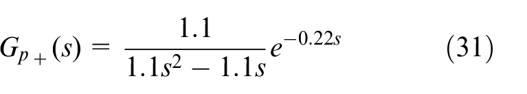
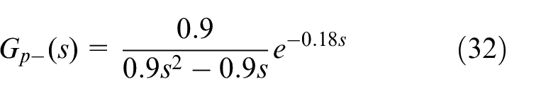
Figure 34 shows the step responses of the +10% perturbed system in equation (31) according to the K f , K d , K p , and K i values obtained for the nominal system using each method. Accordingly, the bar graph of the time domain performance metrics for the step response of each method is given in Figure 35.
Step responses of +10% perturbed system according to K f , K d , K p , K i values obtained for the nominal system using each method for example 4.
Time domain performance metrics for step responses of +10% perturbed system based on K f , K d , K p , K i values obtained for the nominal system using each method for example 4.
Upon examining the servo response of the perturbed system with +10% variation in Figure 34 and the performance metrics obtained from the servo response in Figure 35, it is observed that the methods with the lowest settling time are, respectively STM, WGC and CCSR, with settling times of 4, 4.50, and 5.18 s, respectively. Similarly, for the lowest rise time, the sequence is the CCSR, STM, and WGC methods, with rise times of 0.55, 0.81, and 1.12 s, respectively. However, it’s important to note that while the CCSR method displays a significantly high overshoot, as 18.43%, the WGC and STM methods achieve a comparatively lower level of overshoot, as 7.20% and 8.20%, than CCSR, although they are still relatively high.
Figure 36 shows the servo response of the −10% perturbed system in equation (32) according to the K f , K d , K p , and K i values obtained for the nominal system using each method. Accordingly, the time-domain performance metrics bar graph for the servo response of each method is given in Figure 37.
Step responses of −10% perturbed system according to K f , K d , K p , K i values obtained for the nominal system using each method for example 4.
Time domain performance metrics for step responses of −10% perturbed system based on K f , K d , K p , K i values obtained for the nominal system using each method for example 4.
Based on the examining the servo responses of the perturbed system with a +10% variation in Figure 36 and the performance metrics obtained from the servo response in Figure 37, it is evident that the methods with the lowest settling time and rise time are, in sequence, CCSR, STM, and WGC. The settling times are obtained as 3.29, 4.08, and 4.42 s for CCSR, STM, and WGC, respectively. The rise times are obtained as 0.65, 0.97, and 1.22 s for CCSR, STM, and WGC, respectively. However, it is important to note that while the CCSR method displays an exceedingly high overshoot, as 15.66%, the WGC and STM methods achieve a relatively lower level of overshoot, as 9.09% and 8.39%, compared to CCSR. Furthermore, it is apparent that both WGC and STM methods still exhibit a significant level of overshoot. After conducting these analyses, it can be observed that when PI-PD controllers are designed for a system using these stability region centroid methods, a satisfactory servo and regulatory response is achieved for IUSOPTD. When the reference tracking and disturbance rejection performances of WGC, CCSR, and STM methods have been examined, it is determined that no single method outperforms the others in terms of all performance criteria. Furthermore, upon conducting a robustness analysis, it is evident that all methods maintain stability and yield a successful step response despite variations in system parameters. Upon closer examination of system performance, it becomes apparent that, similar to the nominal system, the methods exhibit advantages and disadvantages in some performance criteria.
Conclusions
This study designed PI-PD controllers with analytical controller tuning methods using the stability region centroid reported in the literature for unstable, integrating and resonant systems with time delay. In the PI-PD control structure, firstly, SBL graphs were obtained for the inner loop containing PD controller of the time-delay systems and K f and K d parameters were obtained according to WGC, CCSR, and STM methods, respectively. According to these K f and K d controller parameters, new transfer functions were obtained in the inner loop and accordingly, a PI controller was designed in the outer loop. PI controller parameters K p and K i were obtained with these three analytical methods, which are also based on the stability region centroid and the closed-loop servo and regulatory responses of the methods were compared. In addition, the disturbance rejection and robustness performances are examined by adding disturbance and parameter changes to the systems. In simulation studies, time domain performance values such as rise time, settling time and maximum overshoot time domain performance values for all cases were obtained and compared. As a result, the analysis shows that a good servo and regulatory response is obtained when PI-PD controllers are designed using these methods for unstable, integrating and resonant systems with time delay. It has been observed that these methods have both advantages and disadvantages concerning some performance criteria in time response analysis. Tracking (servo) and disturbance rejection (regulator) analyses have revealed that none of the methods is entirely superior to the others in terms of all performance criteria. However, it has been observed that they exhibit superior and inferior aspects compared to each other in terms of some time-domain performance criteria. Moreover, robustness analysis showed that all methods maintained closed loop system stability despite the changes in the system parameters and provided a successful step response. Furthermore, during simulations, it has been observed that the application of the methods has both challenges and advantages. Since the PI-PD controller structure is used, it was noted that applying all three methods is more time-consuming compared to designing a PID structure. This is because while only one SBL is used for PID, two separate SBLs are used for PI-PD. However, considering that PI-PD provides more satisfactory results for unstable, integrating and resonant time-delay systems, this drawback can be ignored. Therefore, when examining the methods in PI-PD design, it was found that for the WGC to yield more suitable results, the frequency step size should be selected as small as possible, however excessively small values increase computation time. Hence, it is recommended to choose a reasonable frequency step size (e.g. Δω ≤ 0.01). Moreover, the computation load increased due to the WGC method utilizing points dependent on the entire frequency range to form PI-PD SBLs. However, since software package programs like Matlab are used, this is not a significant disadvantage. In the case of the CCSR method, it was observed that the computational load is lower compared to WGC. Although finding the center point based on observational data may be perceived as a disadvantage, as demonstrated in this study, the application of the CCSR method has been facilitated by using frequency values ω = 0 as the initial frequency, ωmax as the maximum frequency value and ω c frequency values where Kf(ωc) = Kfmax and Ki(ωc) = Kimax with the help of Matlab. The STM has shown similarities to WGC and CCSR in terms of features. However, creating the stability triangle using ω = 0, maximum frequency ωmax and average frequency ωmax/2 has made it easier to implement in Matlab package program. Consequently, this study contributes to the literature by comparing the effectiveness of WGC, CCSR, and STM methods in designing PI-PD controllers for unstable, integrating and resonant systems with time delay. Additionally, when designing PI-PD controllers for unstable, integrating and resonant systems, the STM method has been used for the first time and its effectiveness has been demonstrated. The results presented in this study can be extended for FOPI-FOPD, TID, or FOTID controllers. In future studies, analytical controller design and comparison can be made using methods based on the centroid of the SBL for FOPI-FOPD, TID, or FOTID controllers. Other stability region centroid methods existing in the literature can also be included in the comparison besides these three methods.
Footnotes
Appendix
Abbreviations/Symbols
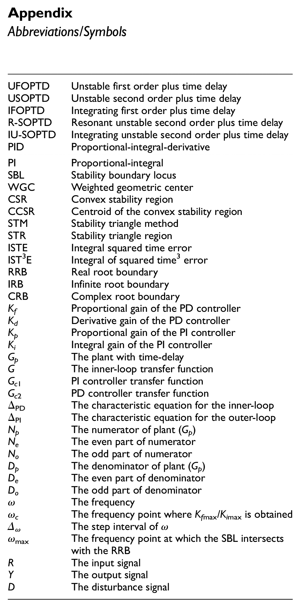
| UFOPTD | Unstable first order plus time delay |
| USOPTD | Unstable second order plus time delay |
| IFOPTD | Integrating first order plus time delay |
| R-SOPTD | Resonant unstable second order plus time delay |
| IU-SOPTD | Integrating unstable second order plus time delay |
| PID | Proportional-integral-derivative |
| PI | Proportional-integral |
| SBL | Stability boundary locus |
| WGC | Weighted geometric center |
| CSR | Convex stability region |
| CCSR | Centroid of the convex stability region |
| STM | Stability triangle method |
| STR | Stability triangle region |
| ISTE | Integral squared time error |
| IST 3 E | Integral of squared time3 error |
| RRB | Real root boundary |
| IRB | Infinite root boundary |
| CRB | Complex root boundary |
| K f | Proportional gain of the PD controller |
| K d | Derivative gain of the PD controller |
| K p | Proportional gain of the PI controller |
| K i | Integral gain of the PI controller |
| G p | The plant with time-delay |
| G | The inner-loop transfer function |
| G c 1 | PI controller transfer function |
| G c 2 | PD controller transfer function |
| ΔPD | The characteristic equation for the inner-loop |
| ΔPI | The characteristic equation for the outer-loop |
| N p | The numerator of plant (G p ) |
| N e | The even part of numerator |
| N o | The odd part of numerator |
| D p | The denominator of plant (G p ) |
| D e | The even part of denominator |
| D o | The odd part of denominator |
| ω | The frequency |
| ω c | The frequency point where K f max/K i max is obtained |
| Δ ω | The step interval of ω |
| ω max | The frequency point at which the SBL intersects with the RRB |
| R | The input signal |
| Y | The output signal |
| D | The disturbance signal |
Acknowledgements
We thank Turkish Academy of Sciences (TÜBA) for supporting this work.
Declaration of conflicting interests
The author(s) declared no potential conflicts of interest with respect to the research, authorship, and/or publication of this article.
Funding
The author(s) received no financial support for the research, authorship, and/or publication of this article.
Data availability statement
Data sharing not applicable to this article as no datasets were generated or analyzed during the current study.