Research on a method of fault identification of rolling bearings based on time series shapelets

Abstract

Recent research on utilizing artificial neural network (ANN) for fault identification of bearings ignores the features of vibration signals as time series, resulting in low interpretability and cannot classify signals of bearing vibration on different dimensions. Time series shapelets is the most identifiable subsequences of time series. Time series can be effectively classified through computing similarities between shapelets and each time series. This paper identifies faulty bearings with a machine learning-based shapelets algorithm, and through modeling, calculation and verification based on CWRU fault bearing data set, some szimportant conclusions are obtained. The results show that this meaningful new method is more accurate and can reduce time consumption compared with traditional time-laboring shapelets, enhancing interpretability of diagnosis in the meantime. Compared with other classification methods, shapelets transforms the classification problem of vibration signal time series into a similarity measurement problem between time series and subsequence shapelets, fully reflecting the essence of bearing vibration signals as a time series. Meanwhile, by using MINDIST distance instead of Euclidean distance in shapelets can effectively reduce the calculation time while ensuring accuracy, which could be a significant method of distance measurement in clustering tasks.

Introduction

Data-driven bearing fault identification methods mainly include support vector machine (SVM) and artificial neural network (ANN), etc. With the fast development of sensor technology, the fault identification method based on condition monitoring gradually replaces the method based on the running time. The problem of the surge in the amount of data caused by this is the focus that academics need to pay attention to in recent years. Cheng et al. ¹ performed local mean decomposition (LMD) on bearing vibration signals, and then extracted time-domain statistics and energy features from the components as input to the neural network to classify faults. Jia ² improved the convolutional neural network with regularized weights and weighted loss functions for the imbalanced sample data set, successfully identifying bearing faults under unbalanced samples, and further researched the physical meanings of the convolution kernel. Hu et al. ³ combined the convolutional neural network with SVM classifier, introducing batch normalization and Dropout processing, and realized high-precision identification of faults of different types and different damage levels.

Methods above are all effective processing methods for massive high-dimensional fault signals, but there are still two shortcomings. First, numerous parameters in math model complicate the optimizing process and the stretched computing time requires more computing power. Second, the model is weakened by low interpretability, ignoring the essence of bearing signal as time series. In order to solve these problems, an algorithm based on subsequences classification called shapelets is introduced to process vibration signals in this paper. The method of shapelets is a classification method based on local features of time series proposed by Ye and Keogh. ⁴ By calculating the similarities between subsequences and the original sequences, K best shapelets subsequences are extracted. The high-dimensional time series would be reduced to K dimensions, and then classified by a 1 -NN classifier or other traditional methods. Jason Lines et al. ⁵ separated the discovery of shapelets from the construction of classifiers, effectively improved the classification accuracy, and retained the original interpretation capabilities of shapelets. Yuan et al. ⁶ proposed a classification method based on logical shapelets transformation, using an intelligent caching based and reusable skill to reduce the time complexity of computing.

In order to overcome the shortcomings such as mode collapse and gradient vanishing, Li et al. ⁷ proposed a supervised model called modified auxiliary classifier GAN (MACGAN) designed with new framework. Compared with the existing GANs, the proposed method can more efficiently generate multi-mode fault samples with higher qualities, which can be used to assist the training of deep learning-based fault diagnosis models with high accuracy and good stability. Xiao et al. ⁸ proposed a novel joint transfer network for unsupervised bearing fault diagnosis from the simulation domain to the experimental domain, and two experimental datasets collected from laboratory test rigs are used as the target domains to validate the effectiveness of the proposed method. The results show that the proposed method is superior to other popular unsupervised cross-domain fault diagnosis methods. The literature ⁹ incorporated the skip-bigram model for the construction of symbiotic word pairs and proposed a novel and fast variable-length word generation method, and used some controlled experiments to verify the effectiveness of the proposed method. Ircio et al. ¹⁰ used an adaptation of existing nonparametric mutual information estimators based on the k-nearest neighbor for the purpose of bringing these methods to the time series scenario, and the results show that the method is able to strongly reduce the number of time series while keeping or increasing the classification accuracy. Compared with two shapelet decision tree models, 1 NN models based on different distance functions, and C4.5 models based on different top-k shapelets transformation algorithms, Wang et al. ¹¹ put forward a lazy classification model, and experimental results show that the proposed model has higher accuracy and stronger interpretability.

In our previous study, ¹² we’ve already discussed the disadvantages of the two current fault diagnosis methods for rolling bearings, which includes over-reliance on signal processing, complicated model and weak interpretability, and so on. Meanwhile, compared with the shortcomings of traditional fault diagnosis technology, the time series classification method based on shapelets learning algorithm can guarantee the accuracy of fault diagnosis while retaining the strong interpretability of shapelets as the most representative time series subsequences. The improvement of the proposed method based on Dropout improved the generalization performance of the model, and achieved 100% diagnostic accuracy on the training and test sets of bearing fault data, which proves the validity of this proposed methods for fault diagnosis of axlebox bearing of EMU.

This paper applied the method of shapelets to classification of faulty bearings, greatly reducing the discovery time of shapelets, which successfully realizes the classification of fault of rolling bearings. This method of shapelets really simplify the optimizing process and the computing power, and have better interpretabilities compared with previous mentioned methods.

Overview of machine learning-based time series shapelets

Introduction of shapelets

D is defined as time series dataset, including n time series: D ={T₁,T₂,…,T _n }. The length of each time series is m, that is T _i ={t_i1,t_i2,…,t _im }. Please refer to Table 1 for symbols used in this paper.

Table 1.

Table of symbols.

Symbol	Meaning
D	Time series dataset
T,R	Time series
s	Subsequences of time series
m, |T|	Length of time series
l, |s|	Length of subsequences
N, | D |	Number of time series
subdist (x,y)	Distance between subsequence and time series
E	Entropy
I	Information gain
G	Split intervals

• Definition 1. Subsequences of time series

For time series $\mathrm{D}=\{T_1,T_2,\dots ,T_n\}$ $\mathrm{T}=\{t_1,t_2,\dots ,t_m\},$ a subsequence of time series is defined as ${\mathrm{S}}_{i,l}=\{t_i,\dots ,t_{i+l-1}\}$ . S is a subsequences of time series T starting from i length of l.

• Definition 2. Entropy

Assuming there are N time series and C categories in the dataset, there are $n_i$ time series of class $c_i$ in D. The entropy of D is defined as:

$$\mathrm{E}\left(\mathrm{D}\right)=-\sum _{i=1}^c\frac{n_i}{N}\log \frac{n_i}{N}$$

(1)

• Definition 3. Measurements of similarity between time series

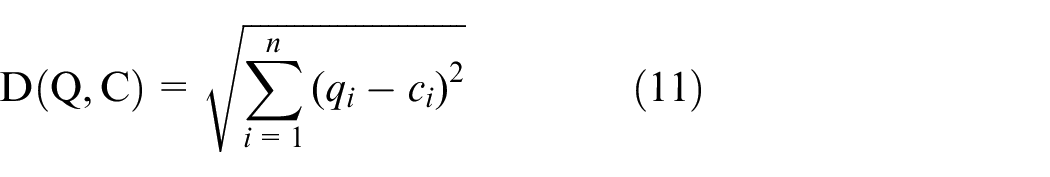
Similarity between time series is measured by distance between each other. For two time series q and c of the same length, Euclidean distance is used to represent the similarity.

For two time series different in length, we slide the shorter time series on the longer time series, and then compute Euclidean distances between the shorter time series and every corresponding segment on the longer time series, of which the minimum value is the subdist of sub-series, that is,

$$\mathrm{subdist}(q,c)=\min (\mathrm{dist}(x,x_{|y|}))$$

(2)

• Definition 4. Split point

Tuple (s,t) is defined as the split point which includes a sub-series s and a distance threshold t. This point splits dataset D into two disjoint subsets, namely $D_{\mathrm{left}}$ and $D_{\mathrm{right}}$ . $D_{\mathrm{left}}=\{x:x\in D,\mathrm{subdist}(s,x)\le t\},$ $D_{\mathrm{right}}=\{x:x\in D,\mathrm{subdist}(s,x)>t\}.$ We use $N_1$ to represent the number of time series in $D_{\mathrm{left}}$ , and $N_2$ to represent the number of time series in $D_{\mathrm{right}}$ .

• Definition 5. Information gain

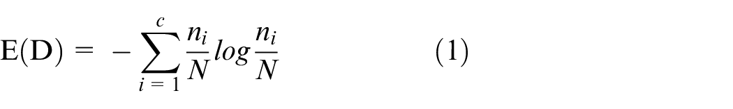
The information gain from splitting D into two disjoint subsets is defined as:

$$\mathrm{I}(\mathrm{s},\mathrm{t})=\mathrm{E}\left(\mathrm{D}\right)-\frac{N_1}{N}E\left(D_{\mathrm{left}}\right)-\frac{N_2}{N}E\left(D_{\mathrm{right}}\right)$$

(3)

• Definition 6. Split interval

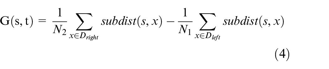
The split interval of a split point is defined as:

$$\mathrm{G}(\mathrm{s},\mathrm{t})=\frac{1}{N_2}\sum _{x\in D_{\mathrm{right}}}\mathrm{subdist}(s,x)-\frac{1}{N_1}\sum _{x\in D_{\mathrm{left}}}\mathrm{subdist}(s,x)$$

(4)

• Definition 7. Shapelet

Shapelet is a tuple (s,t) which consists of subsequences s of T and threshold t. For a classification task, shapelets work to minimize the distance between subsequences of the same class and maximize the distance between subsequences of different classes.

For all the candidate shapelets, we need to sort them to prioritize the shapelet with larger information gain. If the information gains are equal, we prioritize the shapelet with larger split interval. If the split intervals are equal, we prioritize the shorter shapelet. If the lengths are the same, we prioritize the first generated shapelet. Generally speaking, we select shapelets from the perspective of information gain, split interval, length and extracting order.

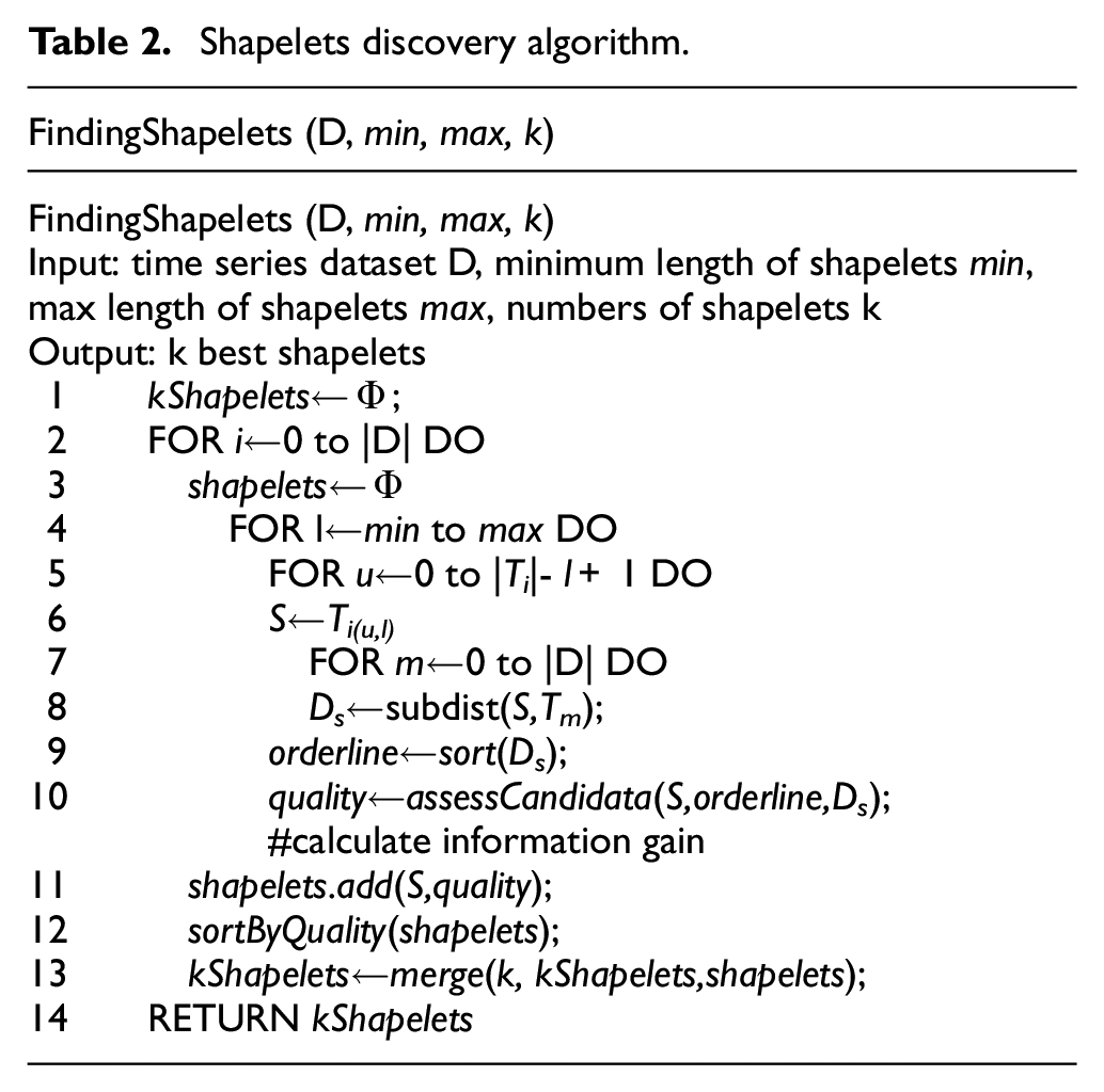
A data transformation algorithm based on regularized Euclidean distances between sub-series and shapelets has been proposed. It also summarized algorithms for shapelets discovery, which is shown in Table 2.

Table 2.

Shapelets discovery algorithm.

FindingShapelets (D, min, max, k)
FindingShapelets (D, min, max, k) Input: time series dataset D, minimum length of shapelets min, max length of shapelets max, numbers of shapelets k Output: k best shapelets
1  kShapelets←Φ;
2  FOR i←0 to |D| DO
3   shapelets←Φ
4    FOR l←min to max DO
5     FOR u←0 to |T i |- l+ 1 DO
6     S←Ti(u,l)
7      FOR m←0 to |D| DO
8      D s ←subdist(S,Tm);
9     orderline←sort(D s );
10     quality←assessCandidata(S,orderline,Ds); #calculate information gain
11   shapelets.add(S,quality);
12   sortByQuality(shapelets);
13   kShapelets←merge(k, kShapelets,shapelets);
14  RETURN kShapelets

Improvements of shapelets

Instead of discovering shapelets, Josif Grabocka et al. ¹³ proposed a method of learning shapelets from time series. There are mainly two steps in this theory. Firstly, roughly estimated shapelets would be randomly got from subsequences, and then, a loss function is built so that the formal candidate shapelets would be optimized iteratively while minimizing the loss function, which is a method used in machine learning.

For a binary classification task, results could be defined as $\mathrm{Y}\in \{0,1\}$ . The predicted classification results of time series can be calculated by a linear function of the similarity measures between k shapelets and each time series, which could be got in section 2.1. So that the prediction result of the i-th time series can be calculated by (4):

$$\widehat{Y_i}=M_0+\sum _{k=1}^K{M}_{i,k}{W}_k$$

(5)

$W_0$ is the bias term and $W_k$ is the weight.

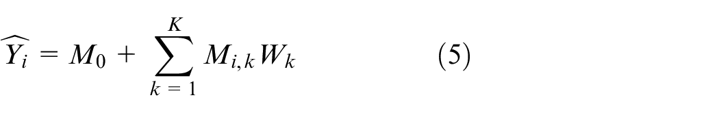
Equation (5) defines a loss function to measure the gap between the actual result and the predicted result.

$$\mathrm{L}(\mathrm{Y},\hat{Y})=-\mathrm{Y}·\ln \mathrm{\sigma }\left(\hat{Y}\right)-(1-\mathrm{Y})·\ln \mathrm{\sigma }(1-\hat{Y})$$

(6)

The $\mathrm{\sigma }$ -function is a logistic function, which maps the independent variables to the interval (0,1):

$$\mathrm{\sigma }\left(\mathrm{Y}\right)=\frac{1}{1+e^{-Y}}$$

(7)

Therefore, the task has been transformed into another task of minimizing the loss function, and the back-propagation algorithm is used to continuously update the bias terms $W_0$ and weights $W_k$ . The optimal $W_0$ and $W_k$ can be obtained through multiple iterations at a certain learning rate, reducing the difference between the actual classification result and the prediction result gap to achieve the purpose of improving the accuracy of classification.

The network structure is shown in Figure 1.

Figure 1.

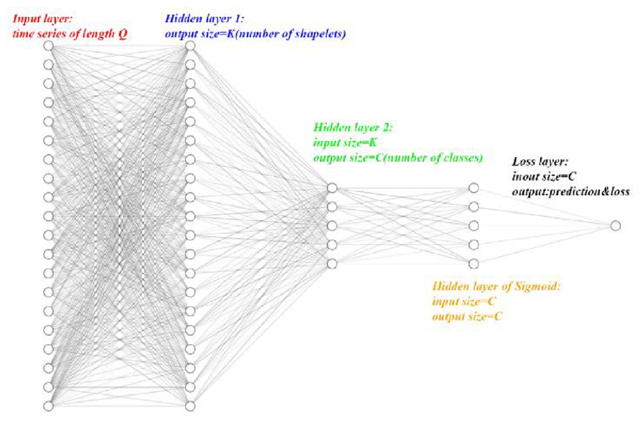
The structure of network is consisted of five layers: one input layer, two hidden layers, one loss layer and one output layer. High-dimensional time series will reduce their dimensions after passing through the network.

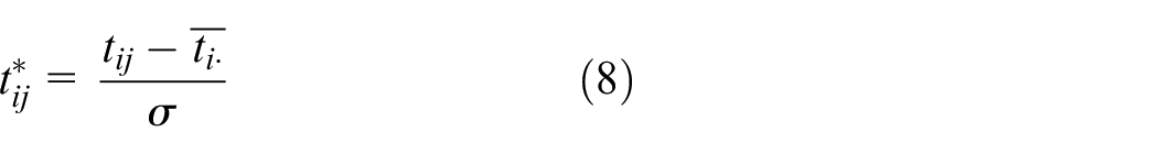
Furthermore, in order to speed up convergence and improve the prediction accuracy of the model, pre-processing of data need to be done. In this paper, a method of z-score (zero- mean normalization) is applied to the original data to make the converted time series mean 0 and standard deviation 1, where (8) is used for a time series $T_i=\{t_{i1},t_{i2},\dots ,t_{\mathrm{im}}\}$ .

$$t_{\mathrm{ij}}^{*}=\frac{t_{\mathrm{ij}}-\overline{t_{i·}}}{\sigma }$$

(8)

$\mathrm{\sigma }$ is the standard deviation of the original time series; $\overline{t_{i·}}$ is the mean value of the original time series.

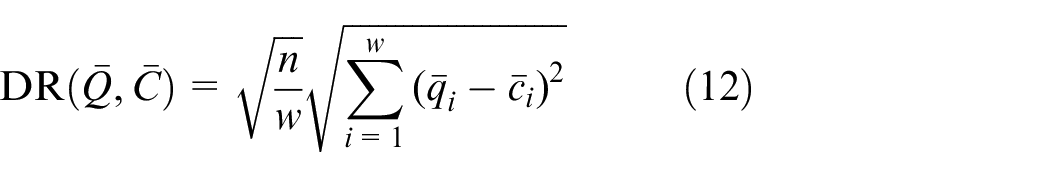
Another method to reduce time consumption is to change the measurement of similarity between subsequences and time series. In this paper, a distance representation is applied instead of traditional Euclidean distance.

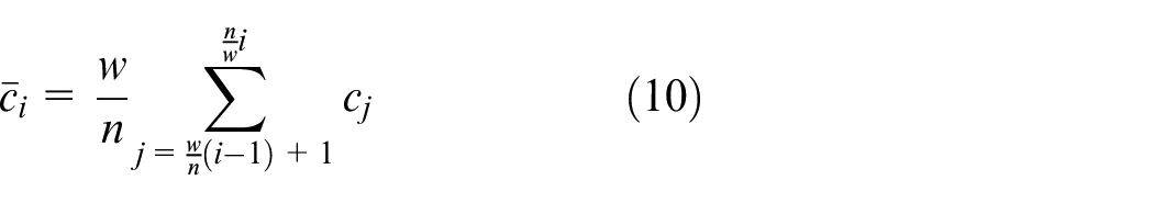
Symbolic representation of time series (SAX) is a quick distance representation proposed by Jessica Lin et al. ¹⁴ In this theory, any normalized time series meets the Gaussian distribution. By piecewise aggregation approximation (PAA), the normalized time series C of length n can be dimensionally exchanged to length of w, which can be represented as:

$$\overline{\mathrm{C}}={\overline{c}}_1+{\overline{c}}_2+\dots +{\overline{c}}_w$$

(9)

The i-th element of $\overline{C}$ is:

$${\overline{c}}_i=\frac{w}{n}\sum _{j=\frac{w}{n}(i-1)+1}^{\frac{n}{w}i}{c}_j$$

(10)

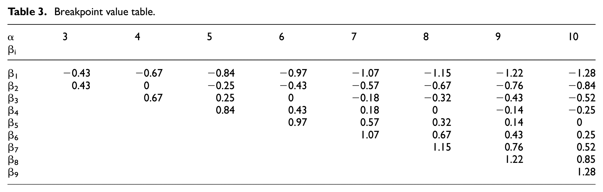
Breakpoints are defined as B = β ₁ , β ₂ ,…, β_α-1, so that in a Gaussian distribution curve, the area under the curve in the interval (β _i , β _i+1 ) is 1/α, among which β ₀ and β _α are defined as negative infinity and positive infinity. The changes in the value of β _i with the value of α are shown in Table 3.

Table 3.

Breakpoint value table.

αβi	3	4	5	6	7	8	9	10
β1	−0.43	−0.67	−0.84	−0.97	−1.07	−1.15	−1.22	−1.28
β2	0.43	0	−0.25	−0.43	−0.57	−0.67	−0.76	−0.84
β3		0.67	0.25	0	−0.18	−0.32	−0.43	−0.52
β4			0.84	0.43	0.18	0	−0.14	−0.25
β5				0.97	0.57	0.32	0.14	0
β6					1.07	0.67	0.43	0.25
β7						1.15	0.76	0.52
β8							1.22	0.85
β9								1.28

SAX is the symbolic representation of time series based on PAA, which defines an alphabet with α symbols: A={A₁, A₂, A₃,…A_α}={a, b, c, …A_α}. For data after PAA processing, when the data point is within the interval of (β _i , β _i+1 ), this data point is represented as the letter A _i . For example, when α = 9, the data of −0.82 is in the interval of (−0.84,−0.52), which can be represented as c. We take a time series from faulty bearings as example, so that IT can be represented as a sentence of ggegdfcgefgeeedegffeddeheefdeehefecfffdg.

SAX processing of this time series is shown as Figure 2.

Figure 2.

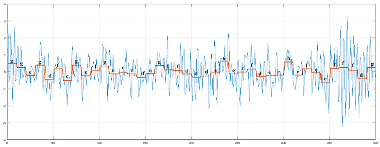
The SAX processing of time series is another method to reduce the dimension and retains local characteristics of time series.

The traditional clustering algorithm mainly calculates the Euclidean distance between sequences and obtains the similarity to achieve clustering.

The SAX method provides a method called MINDIST to achieve this purpose.

For two time series Q and C of length n, the Euclidean distance of the two series can be represented as:

$$\mathrm{D}(\mathrm{Q},\mathrm{C})=\sqrt{\sum _{i=1}^n{(q_i-c_i)}^2}$$

(11)

After PAA processing, the distance between $\overline{Q}$ and $\overline{C}$ is:

$$\mathrm{DR}(\overline{Q},\overline{C})=\sqrt{\frac{n}{w}}\sqrt{\sum _{i=1}^w{({\overline{q}}_i-{\overline{c}}_i)}^2}$$

(12)

After SAX processing, the distance between two “words” or “sentences” can be represented as:

$$\mathrm{MINDIST}(\hat{Q},\hat{C})=\sqrt{\frac{n}{w}}\sqrt{\sum _{i=1}^w{(\mathrm{dist}({\hat{q}}_i,{\hat{c}}_i))}^2}$$

(13)

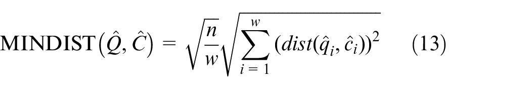
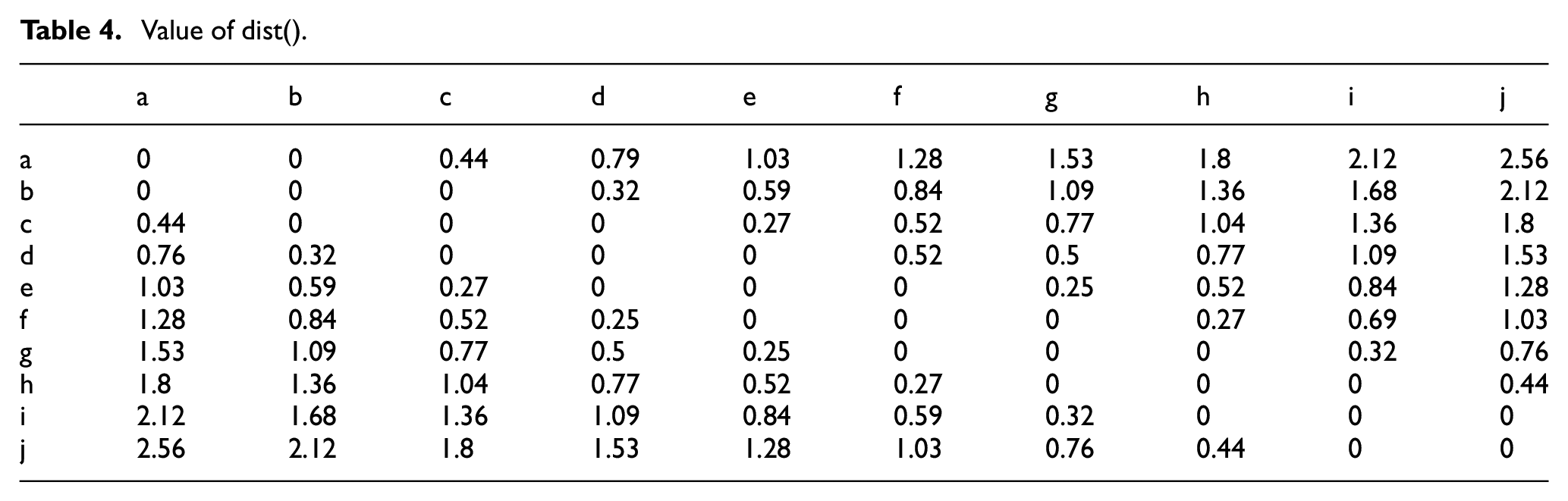
The function of dist() is used to calculate the distance between two letters. The function of local() is defined to represent the location of the letter in the alphabet. For example, if the alphabet is {a, b, c, d, e, f, g}, local(a) = 1,

local(g) = 7. The value of dist() can be obtained from (14).

$$\begin{array}{c}\multicolumn{1}{c}{\mathrm{dist}(\hat{q},\hat{c})=}\\ \multicolumn{1}{c}{\{\begin{array}{c}0,\mathrm{if}|\hat{\mathrm{q}}-\hat{\mathrm{c}}|\le 1\hfill \\ \multicolumn{1}{c}{{\mathrm{\beta }}_{\max (\mathrm{local}\left(\hat{\mathrm{q}}\right),\mathrm{local}(\hat{\mathrm{c}}))-1}-{\mathrm{\beta }}_{\min (\mathrm{local}\left(\hat{\mathrm{q}}\right),\mathrm{local}(\hat{\mathrm{c}}))-1,}\mathrm{others}}\end{array}}\end{array}$$

(14)

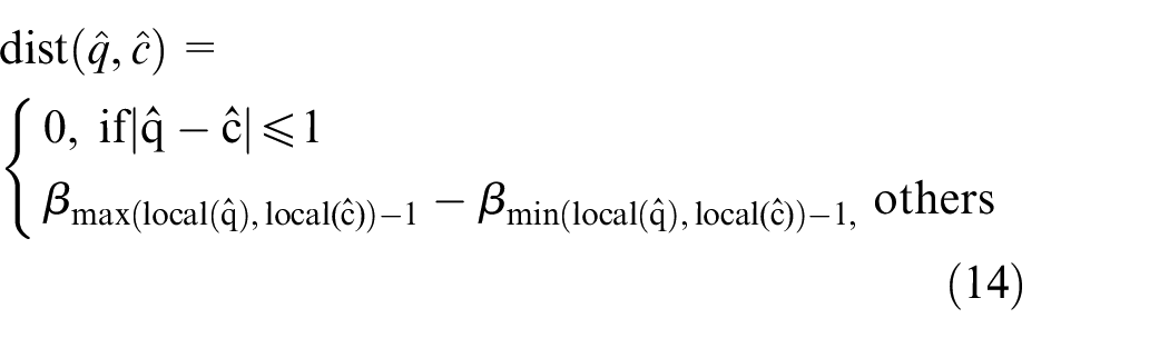
In this paper, the value of α is fixed as 9. The value of dist() is shown as Table 4.

Table 4.

Value of dist().

	a	b	c	d	e	f	g	h	i	j
a	0	0	0.44	0.79	1.03	1.28	1.53	1.8	2.12	2.56
b	0	0	0	0.32	0.59	0.84	1.09	1.36	1.68	2.12
c	0.44	0	0	0	0.27	0.52	0.77	1.04	1.36	1.8
d	0.76	0.32	0	0	0	0.52	0.5	0.77	1.09	1.53
e	1.03	0.59	0.27	0	0	0	0.25	0.52	0.84	1.28
f	1.28	0.84	0.52	0.25	0	0	0	0.27	0.69	1.03
g	1.53	1.09	0.77	0.5	0.25	0	0	0	0.32	0.76
h	1.8	1.36	1.04	0.77	0.52	0.27	0	0	0	0.44
i	2.12	1.68	1.36	1.09	0.84	0.59	0.32	0	0	0
j	2.56	2.12	1.8	1.53	1.28	1.03	0.76	0.44	0	0

Keogh et al. ¹⁵ has proved that the distance of MINDSIT is a lower-bounding distance measurement than Euclidean distance, which deduces false positive and negative errors during clustering. Simultaneously, when processing high-dimensional time series data, the time consumption of MINDIST is much less.

Modeling and validation based on CWRU dataset

The modeling data is from CWRU open source dataset of faulty bearings. Data is acquired from an experiment, the test of which is composed of a motor, a torque transducer a dynamometer and control electronics. Faults of the bearings are artificially applied to the inner race, outer race and the ball by electro-discharge machining with diameters of 7mils, 14 mils and 21 mils. among which, the outer faults are placed a the position of 3 o’clock, 6 o’clock and 12 o’clock. Motor speed used in the experiment includes 1797 rpm, 1772 rpm, 1750 rpm and 1730 rpm. Data has been collected at a sampling frequency of 12,000 Hz and 48,000 Hz. According to the position and the diameters, faults of bearings can be classified into 10 categories: minor inner fault, moderate inner fault, severe inner fault, minor outer fault, moderate outer fault, severe outer fault, minor ball fault, moderate ball fault, severe ball fault and normal bearings.

In this paper, data of the motor speed of 1797 rpm collated at the sampling frequency of 12,000 Hz is adopted to establish the model and the outer faults of bearing are fixed in the position of 6 o’clock. Faults at 1730 rpm motor speed are used later as the validation dataset to verify the generalization ability of the model. To reduce the complexity of the algorithm and to ensure that each time series contains all local features in at least one rotation period the bearings, original signal is intercepted at every 400 data points. The time-domain waveforms of 10 classes of fault are shown in Figure 3.

Figure 3.

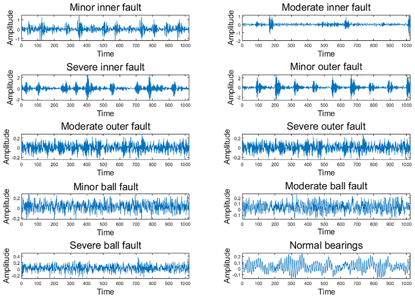
The time domain signal waveform diagram of 10 bearing failure types.

Statistical evaluation of classification model performance

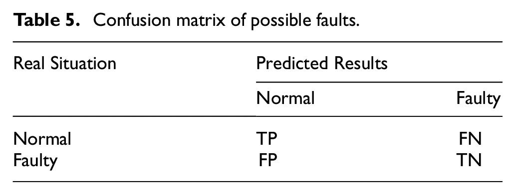
For any binary problem, there are for possible combinations of the classified real situation and predicted results: True Positive (TP), False Positive (FP), True Negative (TN) and False Negative (FN). The confusion matrix of possible faults is as shown in Table 5.

Table 5.

Confusion matrix of possible faults.

Real Situation	Predicted Results
	Normal	Faulty
Normal	TP	FN
Faulty	FP	TN

Accuracy refers to the proportion of the number of correctly classified samples in the total test set samples in all test set data:

$$\mathrm{Accuracy}=\frac{\mathrm{TP}+\mathrm{TN}}{\mathrm{TP}+\mathrm{FN}+\mathrm{FP}+\mathrm{TN}}$$

(15)

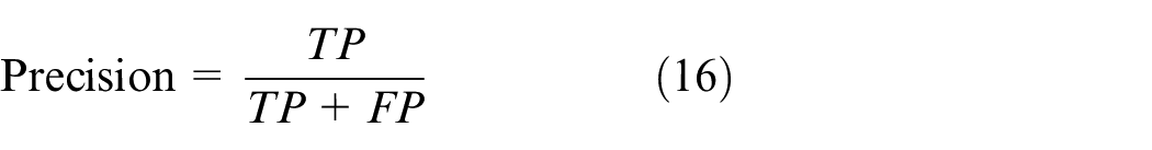
Precision refers to the proportion of the number of true positive samples in the positive samples:

$$\mathrm{Precision}=\frac{\mathrm{TP}}{\mathrm{TP}+\mathrm{FP}}$$

(16)

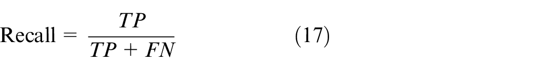
Recall refers to the proportion of the number of correctly classified true positive samples in the actual positive sample:

$$\mathrm{Recall}=\frac{\mathrm{TP}}{\mathrm{TP}+\mathrm{FN}}$$

(17)

F-Measure is the comprehensive consideration of Recall and Precision, which is defined as the weighted harmonic mean of Recall and Precision:

$$\mathrm{F}=\frac{({\alpha }^2+1)P\times R}{{\alpha }^2(P+R)}$$

(18)

When $\mathrm{\alpha }=1$ , F1-Measure is defined as the following formula:

$$\mathrm{F}1=\frac{2\times P\times R}{P+R}$$

(19)

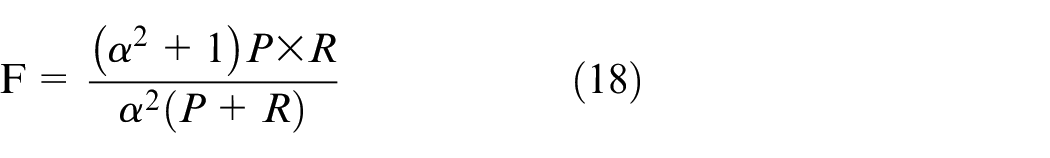
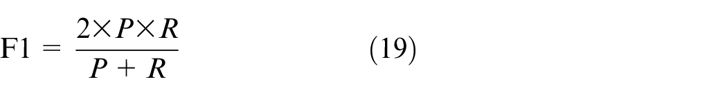
When dealing with multi-classification problems, any two types of failures can be combined to obtain several sets of two-class confusion matrices, and the averages of recall and precision can be obtained. The higher the F1 value, the better the performance of the model would be.

Fault identification experiment

In this section, the method of shapelets is used to identify the location of fault. In order to find early failures in time, data of normal bearings, minor ball faulty bearings, minor inner faulty bearings and minor outer faulty bearings are needed. Model is established by the algorithm of Table 2–2, which is composed of 50 time series for each fault in both training set and test set. Lost function is defined as (5) and SAX distance replaces Euclidean distance to reduce calculation time consumption of time series similarity.

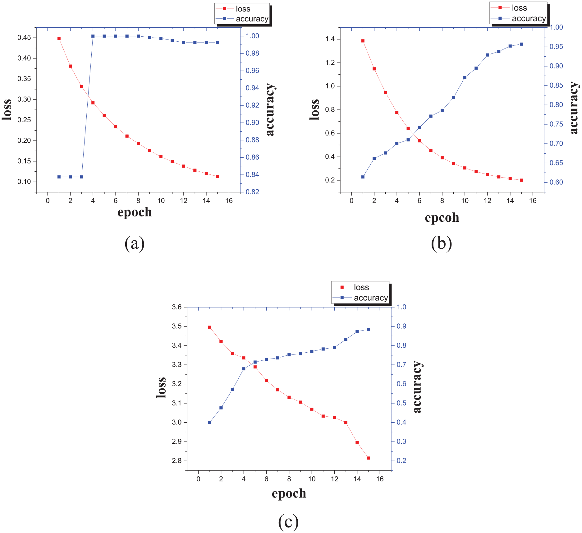
The variation of classification accuracy and loss function with the number of iterations is shown in Figure 4.

Figure 4.

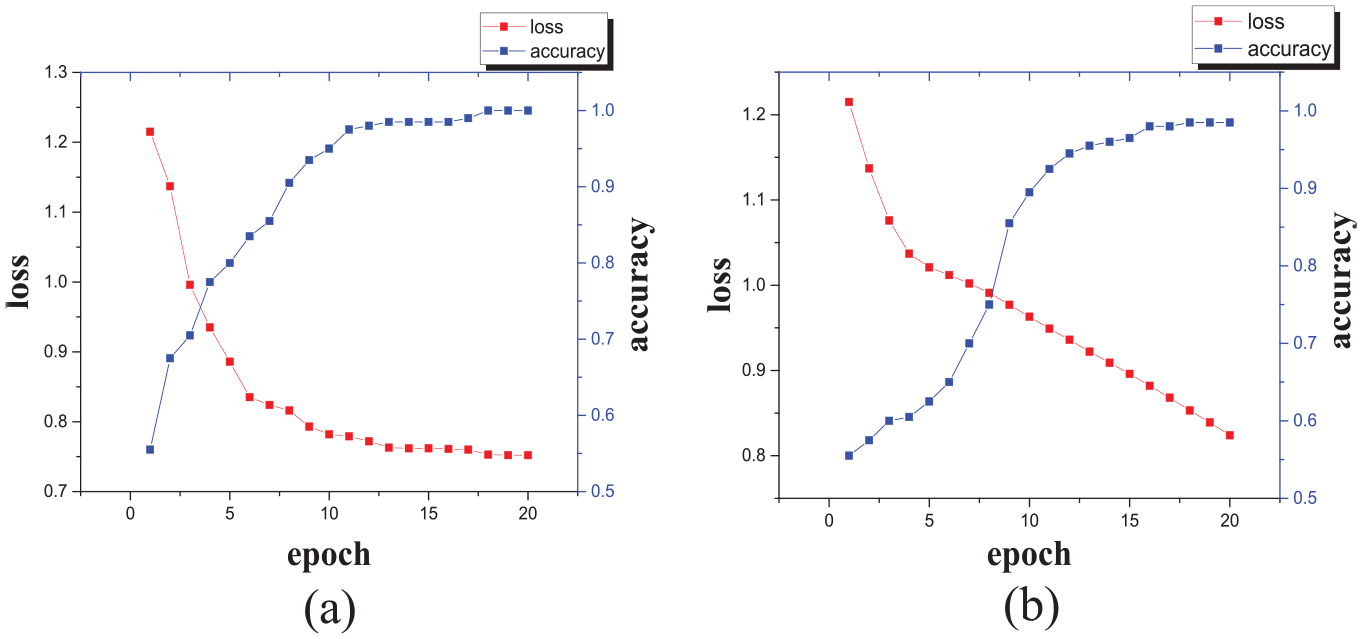
Variation of accuracy and loss function with iterations is as shown: (a) is the result of the use of Euclidean distance and (b) is the result of SAX distance.

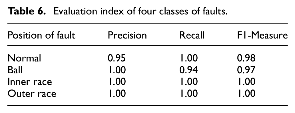
The fault diagnosis accuracy of each task has been verified repeatedly for about 200 times, and the value of Precision, Recall and F1-measure are shown in Table 6, and the time consumption comparison is shown in Table 7.

Table 6.

Evaluation index of four classes of faults.

Position of fault	Precision	Recall	F1-Measure
Normal	0.95	1.00	0.98
Ball	1.00	0.94	0.97
Inner race	1.00	1.00	1.00
Outer race	1.00	1.00	1.00

Table 7.

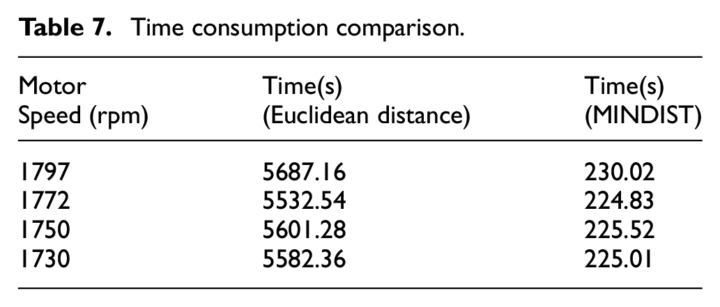
Time consumption comparison.

Motor Speed (rpm)	Time(s) (Euclidean distance)	Time(s) (MINDIST)
1797	5687.16	230.02
1772	5532.54	224.83
1750	5601.28	225.52
1730	5582.36	225.01

The 24 best shapelets are shown in Figure 5.

Figure 5.

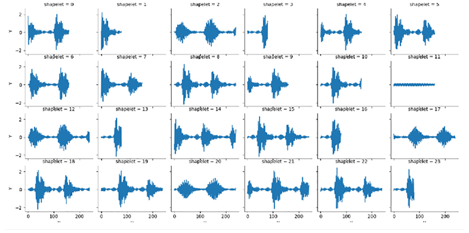
The 24 best shapelets are extracted by the above method.

The purpose of using MINDIST distance instead of Euclidean distance is to reduce time consumption. Therefore, we compared the classification time according to the fault location at different motor speeds. The comparison results are shown in the following table.

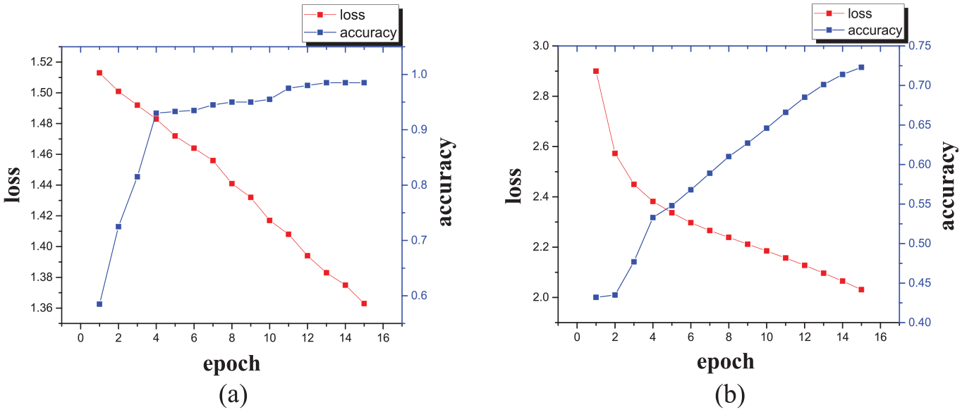
For the problem of if there is a failure or not (two classes) and the level of faults (three class),we also use the same method to test. Furthermore, if different levels of faults in different locations are considered as an independent fault, it would be a classification task of 10 classes, which has also been finished in this section. Results are shown in Figure 6.

Figure 6.

Variation of accuracy and loss function with iterations is shown, which includes two-class task, three-class task and 10-class task: (a) two-class task, (b) three-class task, and (c) 10-class task.

Validation of generalization ability

The generalization ability refers to the ability of the model to adapt to fresh samples, that is, the ability to deal with new datasets with similar laws through the learning of the original dataset. In this section, the bearing vibration signal dataset at the drive end motor speed of 1730 rpm is selected as the validation set to verify the generalization performance of the two-class and multi-class models of the 1797 rpm motor speed vibration signal data set. There are 10 types of faults in the 10-class classification task, including normal bearings, and each type of fault contains 100 time series. The change trend of loss function and classification accuracy with the number of iterations is shown in Figure 7, and the 12 best shapelets are shown in Figure 8.

Figure 7.

Validation result of multi-class task is as shown. When dealing with task of multi-class task, especially when the number of categories is big, the identification result is not good but is still around the percentage of 75%: (a) validation of two-class task and (b) validation of 10-class task.

Figure 8.

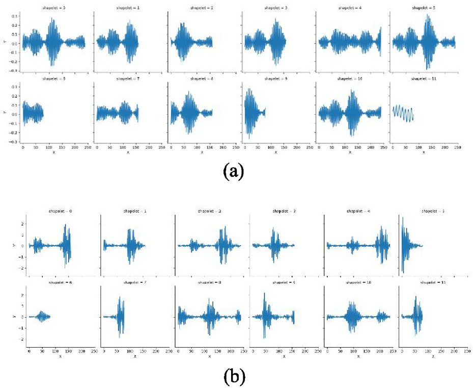
12 best shapelets in validation of multi-class task are shown: (a) 12 best shapelets of two-class classification in validation task and (b) 12 best shapelets of 10-class classification in validation task.

Discussion

For a two-class identification of fault, the evaluation indicators clearly show the high accuracy of this method. The use of SAX distance can greatly save time but the convergence of the model is slower to some extent, which is not a big problem compared to time consumption.

For a multi-class identification, as the number of faults increases, the accuracy of fault identification and the convergence rate of the model decrease. This is a normal phenomenon mainly occurred for two reasons. Firstly, it is an inevitable result of the increase in the amount of data, and secondly, due to the inaccurate measurement in the original data, aliasing phenomenon in time domain representation of different types and degrees of faults is hard to eliminate.

For a practical task of fault identification of bearings, the heart of the problem lies in the discovery of early failures. Any bearing with early failure is not allowed to continue working, which means the decrease of the accuracy of fault identification and the convergence rate when dealing with multi-class identification problem is not a big deal in engineering practice. Actually, the focus is on the position of faults and the above content of this paper has explained the reliability for fault diagnosis of shapelets method when the number of categories is small.

Conclusion

This paper first applied shapelets-based time series classification method to the field of bearing fault identification. Through modeling, calculation and verification based on CWRU fault bearing data set, the conclusion is as follows:

• (1) Shapelets-based time series classification method is a feasible method for bearing fault identification with high classification accuracy, strong comprehensive performance of the model, and strong generalization ability when dealing with classification problems with a small number of categories. It can achieve high-precision diagnosis of faulty bearings under different working conditions.

• (2) This method has been proved to be of high interpretability. Compared with other classification methods, shapelets transforms the classification problem of vibration signal time series into a similarity measurement problem between time series and subsequence shapelets, fully reflecting the essence of bearing vibration signals as a time series.

• (3) Using MINDIST distance instead of Euclidean distance in shapelets can effectively reduce the calculation time while ensuring accuracy, which could be a significant method of distance measurement in clustering tasks.

• (4) The reduction of the model’s convergence speed caused by the use of MINDIST distance and the reduction of the accuracy of multi-classification tasks are the main problems that this method needs to solve in the future.

• (5) More effort needs to be done to improve the generalization performance of the model as the current model can be used to achieve a specific length of time series classification. Furthermore, when shapelets have been extracted, it is possible to realize the Real-time diagnosis and classification of fault signals, which also needs the assistance of hardware including sensors to collect acceleration signals. It is also a meaningful topic that the whole system can be designed with FUSA function.