
Abstract
The classical distributed hybrid flow shop scheduling problem (DHFSP) only considers static production settings while ignores operation inspection and reprocessing. However, in the actual production, the manufacturing environment is usually dynamic; and the operation inspection and reprocessing are very necessary to avoid unqualified jobs from being transported to other production units and to make reasonable arrangements for unqualified and unprocessed jobs. In this paper, we propose a DHFSP with operation inspection and reprocessing (DHFSPR) for the first time, in which the operation inspection and reprocessing as well as the processing time and energy consumption are considered simultaneously. An improved memetic algorithm (IMA) is then designed to solve the DHFSPR, where some effective crossover and mutation operators, a new dynamic rescheduling method (DRM) and local search operator (LSO) are integrated. A total 60 DHFSPR benchmark instances are constructed to verify the performance of our IMA. Extensive experiments carried out demonstrate that the DRM and LSO can effectively improve the performance of IMA, and the IMA has obvious superiority to solve the DHFSPR problem compared with other three well-known algorithms. Our proposed model and algorithm here will be beneficial for the production managers who work with distributed hybrid shop systems in scheduling their production activities by considering operation inspection and reprocessing.
Keywords
Introduction
Most recently, the distributed hybrid flow shop scheduling problem (DHFSP) has attracted an increasing number of researchers and production managers due to the economic globalization and increase of personal and diversity requirements of customers. The DHFSP entails arranging jobs, factories, workshops, machines appropriately to generate feasible solutions,1–5 which includes four sub-problems: (1) assigning each job to a factory selected from the optional factory set; (2) assigning each job to a workshop selected from the optional workshop set from a corresponding factory; (3) assigning each job to a machine selected from the optional machine set from a corresponding workshop of factory; and (4) sequencing the operations satisfying the constraints among factories, machines and operations simultaneously. Obviously, the DHFSP is a more difficult NP-hard problem than the traditional flow shop scheduling problem (FSP) with only one factory.6–8
In the recent decade, a various dynamic events have been studied in the production scheduling in recent years: such as new jobs arrival,9–12 uncertain processing times,13–15 machine breakdowns,16–19 operator unavailability,20,21 job cancellation,22–25 etc. However, to the best of our knowledge, in the field of DHFSP, all existing researchers ignored the dynamic events of operation inspection and reprocessing, that is, they assumed that the production process is deterministic and unchanged; but in the real production systems, operation inspection and reprocessing are inevitable. For example, when an operation is finished processing, it is need to be inspected to detect the production defects timely and avoid unqualify products flowing to the next production stage. If the inspection result of the operation is qualified, it can be transported to the next stage for further processing; else if the result is unqualified, the process may be repaired, reprocessed, or directly scrapped, and other unprocessed processes need to be rescheduled.
Facing the above discussed practical production scheduling problem, the production managers must have to face the following situations when making scheduling decisions in the DHFSP:
(1) In actual production, the operation quality may be affected by many uncertain events, such as the uncertainty of material quality, processing methods, and measurement tools. Without inspection, the defective jobs will be transported to the next production stage, which not only delays the completion time, but also adds additional processing, transportation and energy consumption costs. Therefore, how to arrange the operation inspection in each production stage and how to arrange the defective jobs to be reprocessed in the DHFSP is a thorny problem for the production decision makers, considering the operation inspection and job transportation simultaneously.
(2) If the inspection result of an operation of a job is unqualified, it needs to be reprocessed or scrapped, which will make the original scheduling scheme infeasible. Hence, how to arrange the defective jobs to generate a feasible rescheduling scheme is another tough problem for the production decision makers, considering different inspection results of the jobs.
(3) The DHFSP is a more NP-hard problem compared with the traditional FSP, which means that the traditional linear integer programing methods are difficult or even impossible to obtain accurate solutions in finite time. Hence, how to construct an effective optimization algorithm to solve the DHFSP is another important problem for the production decision makers, considering the optimization objectives of maximal completion time and total energy consumption simultaneously.
In addition, memetic algorithm (MA) as one of the most effective multi-objective algorithms, has been extensively applied to solve various scheduling problems in recent years. For instance, Yuan and Xu 26 proposed some new memetic algorithms (MAs) for the multi-objective flexible job shop scheduling problem (FJSP) with the objectives to minimize the makespan, total workload, and critical workload. Gong et al. 27 proposed a novel MA to solvethe classical distributed production scheduling problem, aiming to minimize the makespan and total energy consumption. Luo et al. 28 proposed an efficient MA to solve the distributed flexible job shop scheduling problem with transfers with the objectives of minimizing the makespan, maximum workload, and total energy consumption of factories. To addresses the multi-objective energy-efficient FJSP with type-2 processing time, Li et al. 29 proposed a mixed-integer linear programing model and designed a learning-based reference vector memetic algorithm to solve it. In order to determine the appropriate speed of the machine and the location of maintenance activities, Abedi et al. 30 proposed a multi-population and multi-objective MA, in which the solutions are distributed into sub-populations.
Inspired by the above findings, in this paper, to solve the practical DHFSP with operation inspection, operation reprocessing and operation transportation among different factories, workshops and machines, the following researches were conducted. Firstly, a new model of the DHFSP considering operation inspection and reprocessing (DHFSPR) is proposed to achieve a better production performance. In addition, an improved memetic algorithm (IMA) is proposed to solve the DHFSPR aiming at minimizing the makespan and total energy consumption. In the IMA, a four-layer coding method and a new load balancing initialization method are designed to obtain high quality initial population; some effective crossover and mutation operators and a local search operator (LSO) are presented to obtain a larger solution space and accelerate the IMA’s convergence speed; a new mathematical model of DHFSP with operation inspection and reprocessing (DHFSPR) is proposed to realize a better production scheduling and a comprehensive dynamic rescheduling method (DRM) including three rescheduling strategies is designed to generate rescheduling schemes according to the inspection results of operations. Finally, in the experimental phase, a total of 60 DHFSPR benchmark instances are constructed to test the proposed algorithm, and four sets of experiments are designed to evaluate the effectiveness of the proposed operators and IMA. More specifically, the first experiment is conducted to obtain the optimal parameter combinations of the proposed IMA and other three compared algorithms based on the Taguchi experimental method 31 ; the second and third experiments are used to verify the effectiveness of the LSO and DRM respectively. The fourth set of experiment is carried out to evaluate the effectiveness of the proposed IMA by comparing it with other three well-known multi-objective algorithms.
The contributions of this paper can be summarized as follows:
(1) We proposed a DHFSP model for the first time, which considers both operation and reprocessing. Compared with the traditional HFSP, this model has stronger flexibility and is more suitable for practical production.
(2) An IMA was designed to solve the proposed DHFSP, in which a new well-designed four-layer chromosome coding method, a new load balancing initialization method, some effective crossover and mutation operators, and an LSO were integrated to obtain a high quality initial population, expand the solution space and accelerate the IMA’s convergence speed.
(3) A comprehensive dynamic scheduling strategy that includes three rescheduling methods is provided to minimize the makespan and arrange the reprocessing operations to the idle machines as much as possible based on the event-driven rescheduling strategy and the full rescheduling method in predictive response scheduling.
The rest of this paper is organized as follows. In Section 2, the mathematical model and DRM are introduced in detail. Section 3 introduces the specific structure and content of the IMA. The experimental result and analysis are presented in Section 4. In the end, Section 5 summarizes paper and looks forward to the future research.
Literature review
Related work on DHFSP
Since the DHFSP was first proposed by Ying and Lin, 32 an increasing number of researchers have expanded and studied the problem from multiple aspects. Lu et al. 33 designed a Pareto-based multi-objective hybrid iterated greedy algorithm by integrating the merits of genetic operator and iterated greedy heuristic to consider green goals in a distributed production environment. To minimize the adjustment and energy consumption simultaneously, Mou et al. 34 proposed the energy-efficient distributed permutation flow-shop inverse scheduling problem. Dong and Ye 35 established a distributed two-stage reentrant hybrid flow shop bi-level scheduling model, which takes makespan, total carbon emissions and total energy consumption costs as the optimization objectives. With increasing environmental awareness and energy requirement, Wang and Wang 36 addressed the energy-aware DHFSP with the objectives of minimizing the makespan and energy consumption simultaneously. Yu et al. 37 proposed a mixed integer linear programing (MILP) model and a knowledge-based iterative greedy algorithm considering the production of constrained resources (such as worker resources) in DHFSP. Considering the production of spare parts and the limited number of workers, a collaborative optimization problem of spare parts production and worker arrangement driven by operation and maintenance is proposed by Wang et al., 38 and an improved Non-dominated Sorting Genetic Algorithm-II is proposed to solve it. Shao et al. 39 investigated a distributed heterogeneous hybrid assembly line workshop scheduling problem with energy and labor perception (ELDHHFSP), and proposed MILP model for ELDHHFSP with the goal of minimizing total delay, total production cost, and total carbon emissions. Starting from the solution and strategy space, a network MA for the ELDHHFSP is proposed.
Considering some factors exiting in real production settings, some extend versions of DHFSP were studied by many researchers. To improve the operational efficiency and competitive advantage of supply chains, Qin et al. 40 proposed three fast heuristics (CR-based heuristic, SLACK-based heuristic, and EDD-based heuristic) and an adaptive human-learning-based genetic algorithm to minimize the sum of earliness, tardiness and delivery costs. Cai et al. 41 considered DHFSP with sequence-dependent setup times in which factory assignment and machine assignment of first stage are integrated together. A new shuffled frog-leaping algorithm with memeplex quality is proposed to minimize the total tardiness and makespan simultaneously. Li et al. 42 proposed a hybrid artificial bee colony algorithm to solve a parallel batching DHFSP with deteriorating jobs. More and more enterprises are facing rapidly changing market demands and small yet frequent orders, Shao et al. 43 studied a distributed heterogeneous hybrid flow shop lot-streaming scheduling problem with the minimization objective of makespan.
As mentioned above, the existing researches about DHFSP typically consider the factors in the actual manufacturing systems, such as energy efficiency, worker flexibility, heterogeneous factories, workshops, and transportation. However, to the best of our knowledge, no research about DHFSP considers the operation inspection and reprocessing, while which widely exist in the actual production environments. This may lead to resource waste and make the original plan infeasible. Therefore, to make the DHFSP model more in line with actual production, it is of great significance to study the DHFSP that considers the operation inspection and reprocessing.
Related work on dynamic scheduling
In terms of dynamic FSP (DFSP), Lee and Kim 44 addressed a robotic FSP with processing time variations where two-part types are processed on each given set of dedicated machines and use a reinforcement learning (RL) approach to obtain efficient robot task sequences to minimize the makespan. Marichelvam and Geetha 45 proposed an improved MA to tackle energy-efficient FSPs with uncertainties such as cancelled and new orders to minimize the total energy cost. Considering the dynamic events endanger baseline schedules, which may require a cost intensive re-scheduling, Grumbach et al. 46 provided a novel method for robust-stable scheduling in dynamic flow shops based on deep reinforcement learning (DRL) implemented with OpenAI frameworks. The method is demonstrated using different flow shop instances with uncertain processing times, stochastic machine failures and uncertain repair times.
Regarding to the dynamic job shop scheduling problem (DJSP), Zhang et al. 47 presented a multi-agent manufacturing system based on DRL to solve the DJSP, which integrates the self-organization mechanism and self-learning strategy. Zhang et al. 48 introduced Digital Twin into the DJSP, which can provide more information for predicting machine availability, and help to detect interference by comparing physical machines with constantly updated digital counterparts in real-time, and triggers rearrangements in a timely manner when needed. Since traditional methods cannot dynamically generate effective scheduling strategies in face of the disturbance of environments, Zeng et al. 49 proposed a flexible hybrid framework that takes disjunctive graphs as states and a set of general dispatching rules as the action space with minimum prior domain knowledge. Li et al. 50 presented a modeling and solution approach for a robust DJSP under deterministic and stochastic machine unavailability caused, respectively, by planned preventive maintenance and unplanned corrective maintenance following random breakdowns. Shady et al. 51 proposed a genetic programing approach to generate dispatching rules automatically for multi-objective DJSP considering machine breakdowns. Considering the dynamics and the uncertainties such as machine breakdown and job rework of the job-shop environment, Wang et al. 52 proposed a dynamic scheduling method based on DRL and adopting proximal strategy optimization to find the optimal scheduling strategy to cope with the curse of state.
For the dynamic FJSP (DFJSP), Chang et al. 53 proposed a DRL to solve the DFJSP with random job arrival, with the goal of minimizing penalties for earliness and tardiness. Zhang et al. 54 proposed an effective two-stage algorithm based on convolutional neural network to solve the DFJSP with machine breakdown. Luo et al. 55 proposed a knowledge-driven two-stage MA and used a rescheduling strategy is implemented in the scheduling process to mitigate the impact of machine breakdowns. An et al. 56 studied the DFJSP with new job insertion and machine preventive maintenance (PM), established an imperfect PM (IPM) model, determined the optimal maintenance plan for each machine, and proposed an improved adaptive reference vector non dominated sorting inheritance algorithm III to solve the problem. Zhang et al. 57 proposed a novel multifidelity-based surrogate-assisted genetic programing and proposed an effective collaboration mechanism with knowledge transfer for utilizing the advantages of multifidelity-based surrogate models to solve the desired problems. Due to the real manufacturing system is prone to various disturbance events, which increase the complexity and uncertainty of shop floor, Li et al. 58 adopted deep reinforcement learning to solve the dynamic FJSP with insufficient transportation resources. In the production process of flexible job shop, there are dynamic events such as machine breakdowns or new job arrivals, Duan and Wang 59 proposed a new robust optimization method that considers dynamic events and designs two indicators for evaluating the robustness of the system, namely the reusability of the system and the reproducibility of processing tasks. Wang et al. 60 designed a novel dynamic multi-objective scheduling algorithm based on DRL. The algorithm uses two deep Q-learning networks and a real-time processing framework to process each dynamic event and generate complete scheduling scheme.
From the above, it can be seen that the dynamic scheduling has received an increasing attention from researchers. However, they normally ignore the dynamic events of operation inspection and reprocessing, while which are actually one of the most common dynamic events in real production environments. For example, if the inspection result of a finished operation is unqualified, how will we handle this operation? Reprocessing or scrapping the unqualified operations will result in the original scheduling plan being infeasible, increasing costs, and effect other unprocessed operations. Therefore, it is very necessary to propose intelligent optimization algorithms with high performance and robustness to address the impact of operation reprocessing and scrapping on the production system.
The mathematic model of the DHFSPR
Problem description
The DHFSPR studied in this paper consists of n jobs (J1, J2, …, Jn), f factories (F 1 , F2, …, Ff), each factory contains w workshops (W 1 , W2, …, Ww), each workshop contains m machines (M 1 , M2, …, Mm); and has l production stages {G 1 , G2, …, Gl}. In each stage, the factories, workshops and machines can be randomly selected for the corresponding operations. Each job is processed in the same sequence from G 1 to G l . Depending on the factory, workshop, and machine set, there are multiple parallel machines (M k ≥ 2) in each stage. The DHFSPR model proposed in this paper considers the jobs transportation among different factories, workshops and machines, including two optimization objectives: (1) maximum completion time; and (2) total energy consumption.
The DHFSPR model must meet the following constraints:
All jobs must be processed according to the sequence of stages.
A machine can process only one operation of a job at any time.
Each operation can only be processed on a machine located in a workshop of a factory at the same time.
The operation must be carried out continuously without interruption.
The operations of different jobs have the same priority.
Any operation of a job cannot be processed until its previous operations are finished.
Each operation must be inspected before it can be transported to the next stage for processing.
Inspection time of each operation is predefined.
The processing time of operations of all jobs are predefined.
The unit energy consumption of all machines is set in advance.
Transportation times and energy consumption between different factories, workshops and machines are predetermined.
Parameters and variables
All parameters and symbols in the model of the DHFSPR are shown in Table 1.
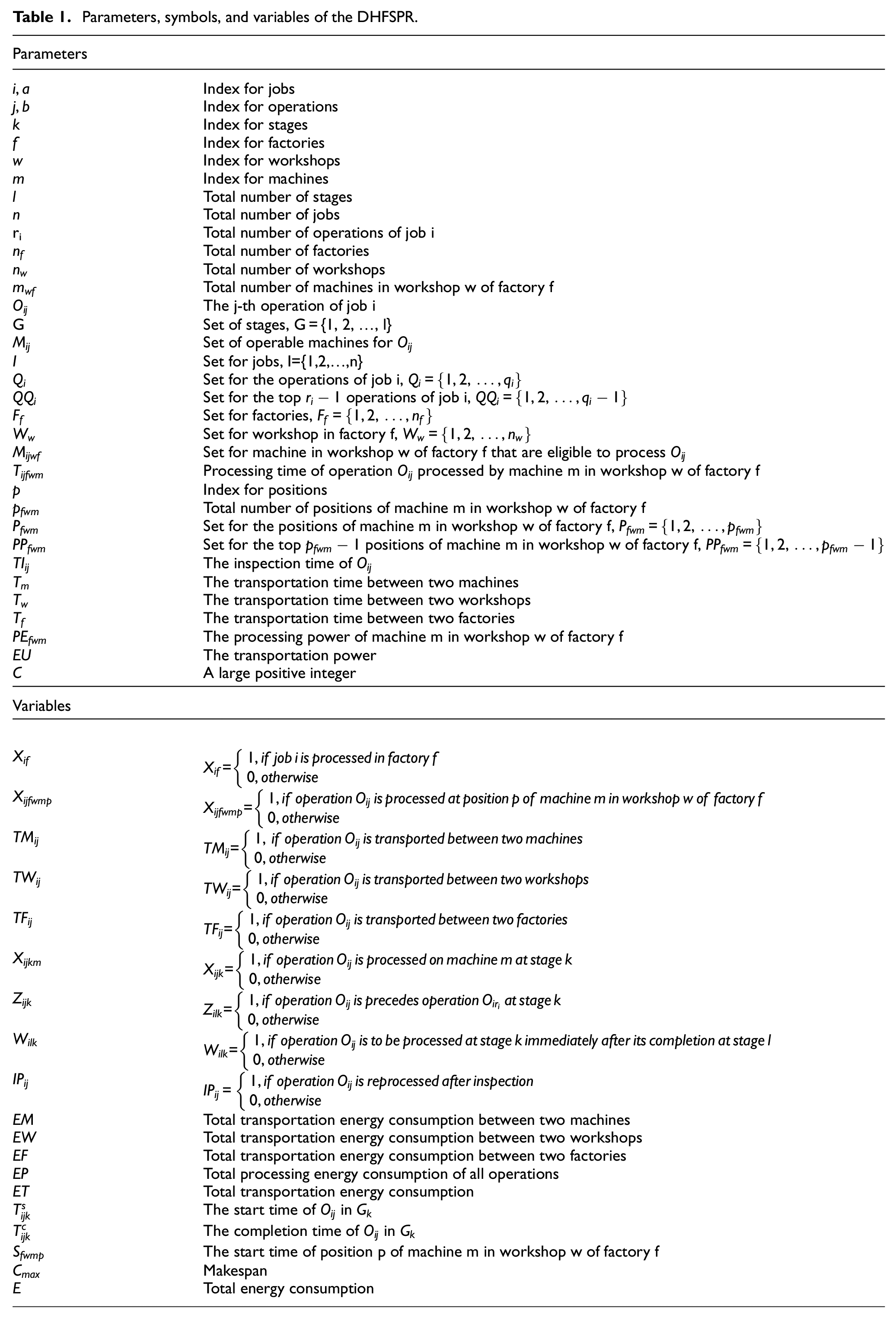
Parameters, symbols, and variables of the DHFSPR.
Energy consumption model
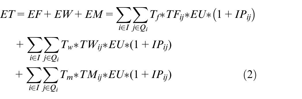
The total energy consumption (E) includes the total energy consumption of machine processing (EC) and total energy consumption of transportation (ET), which are defined as follows:
(1) EC is the total energy consumption of all machines during processing and can be calculated by using equation (1).
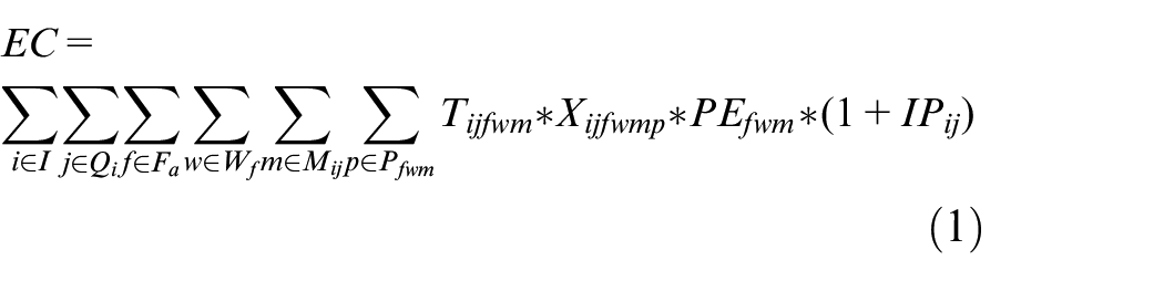
(2) ET is the total energy consumption of all jobs transported among different factories, workshops and machines, and can be calculated by using equation (2).
Mathematical model of DHFSPR
Based on the model in literature 61 and the above parameters and energy consumption model, the mathematical model of DHFJSP is as follows: the above parameters and energy consumption model, the mathematical model of DHFJSP is as follows:
(1) Minimizing the makespan (ob1)

(2) Minimizing the total energy consumption (ob2)


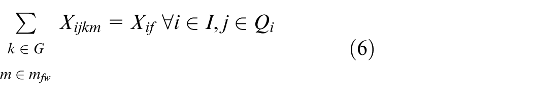
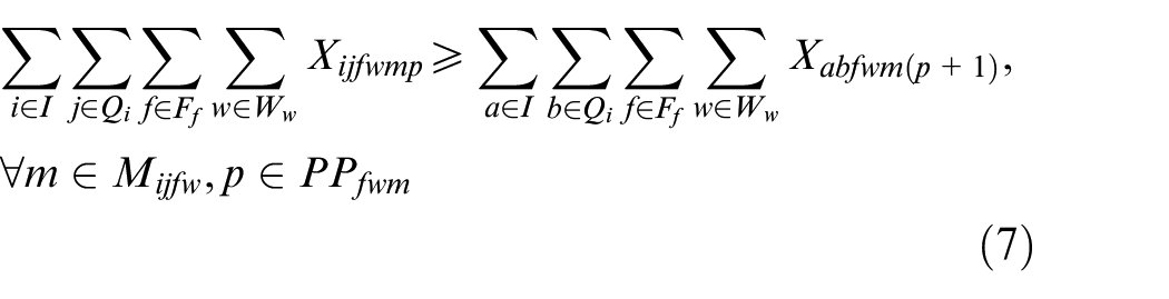
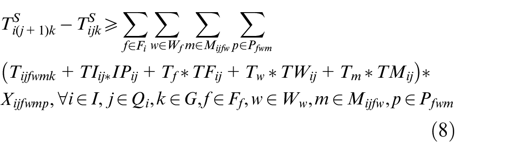
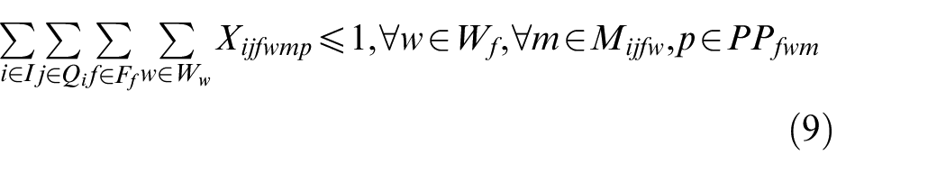
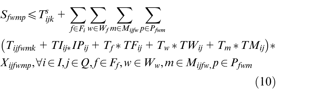


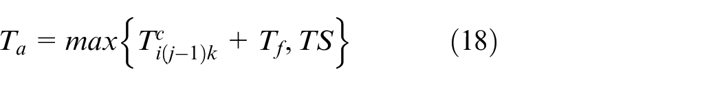
In the above mathematical model, equations (3) and (4) represent the objectives of minimizing the makespan and total energy consumption. Constraint (5) requires that the starting time of a job on the first stage is later than or equal to time zero. Constraint (6) ensures that each job must be processed by any one machine at each stage. Constraint (7) guarantees that the machining position on each machine is determined and must be assigned to the operation sequentially. Constraint (8) specifies the processing sequence between operations of all jobs. Constraints (9)-(10) make sure that at most one operation is scheduled at each position of each machine at the same time, and no overlapping processing is allowed. Constraints (11) defines the completion time of each operation. Constraints (12) ensures that an operation of a job can be started only when the operation at previous stage is finished. Constraint (13) defines the target value of makespan. Constraint (14) guarantees at most one transportation is allowed for each operation among factories, workshops and machines at the same time. Constraints (15)–(17) ensure that the start and finish times of all operations, as well as the start times of all positions, have no variables less than 0.
Model example
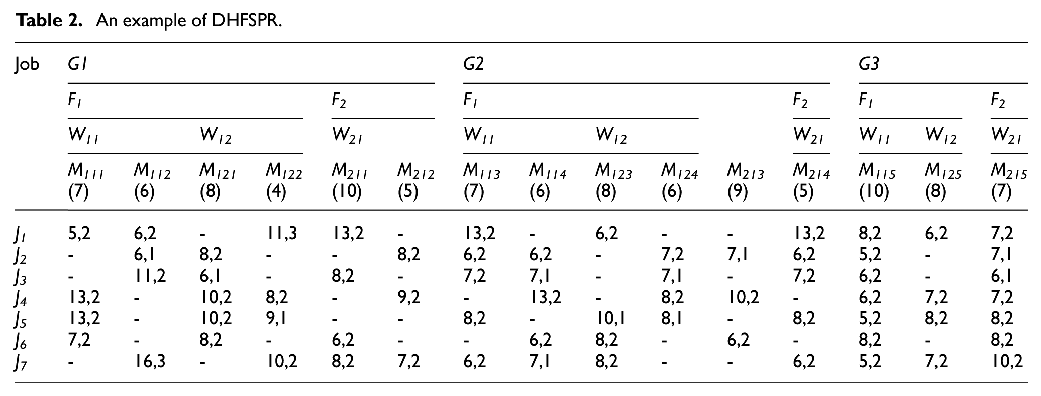
Table 2 shows a simple example of the DHFJSP model, which includes three stages (G1, G2 and G3), seven jobs (J 1 , J2, …, J7) processed in sequence according to the stage sequence, and two factories (F 1 and F 2 ). Taking G1 for example, in which F1 and F2 each have two workshops (W 11 and W 12 ) and one workshop (W 21 ); and W 11 , W 12 and W 21 have two machines (M 111 and M 112 ), two machines (M 121 and M 122 ), two machines (M 211 and M 212 ), respectively. G2 and G3 can be described as G1. The numbers in the brackets indicate the unit processing energy consumption (P Efwm ) of the corresponding machines. The data to the left and right of the comma represent the processing time (T ijfwm ) and inspection time (T Iij ) respectively for the corresponding operations. If we want to get the T ijfwm , T ij and P Efwm of J 1 on M 121 in W 12 of F 1 in G2, we just need to set i = 1, j = 2, k = 2, f = 1, w = 2, m = 2, then T ijfwm = 50, T iij = 18, P Efwm = 6. The dashes in Table 2 (“-”) indicate that their corresponding operations cannot be performed on the corresponding machines. For example, M 111 in W 11 of F 1 cannot process J 1 in G1.
An example of DHFSPR.
Rescheduling method
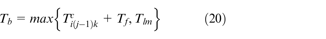
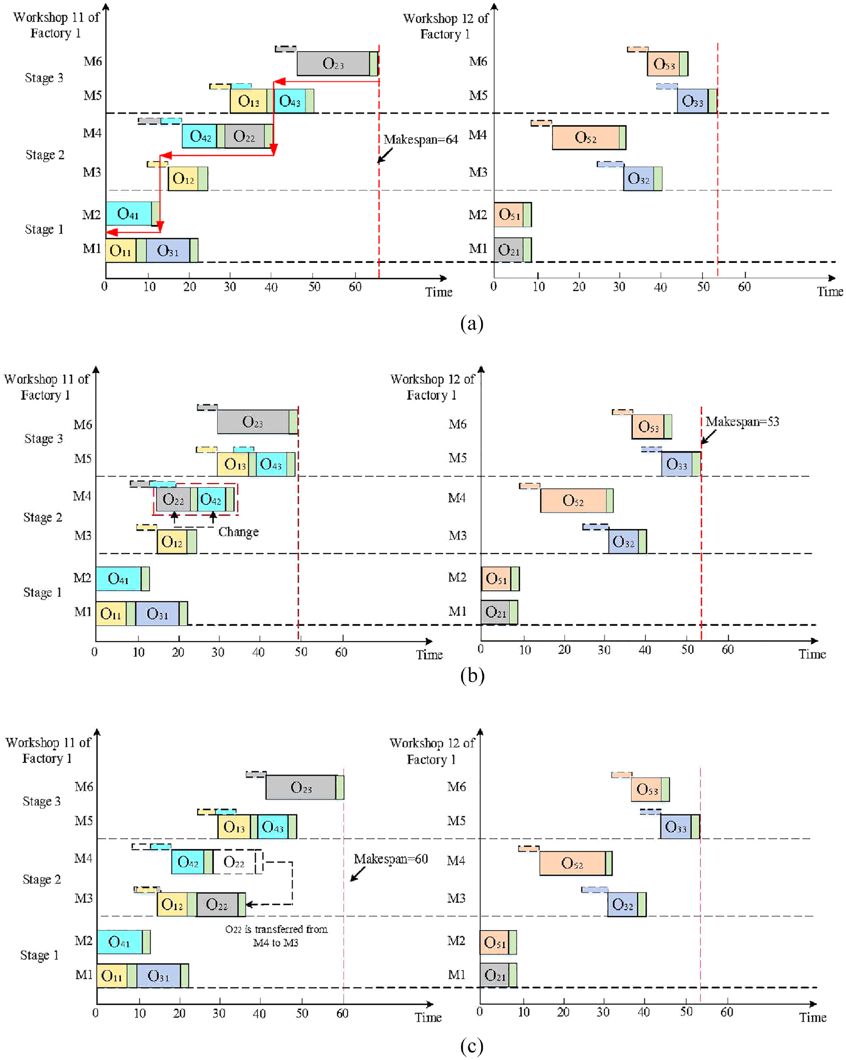
In this paper, a dynamic rescheduling method (DRM) is proposed to minimize the makespan and to arrange the reprocessing operations to the idle machines as much as possible based on the event-driven rescheduling strategy and the full rescheduling method in predictive response scheduling. The DRM includes three strategies which are described as follows, where T ijfwmk and L fwmk represent the reprocessing time of the rescheduled O ij on machine m of workshop w of factory f in stage k and the interval length between two adjacent operations on machine m of workshop w of factory f in the stage k, respectively.
To illustrate the rescheduling process clearly, Figure 1 shows a Gantt chart of a rescheduling scheme for operation reprocessing, in which the green and red squares adjacent to operations indicate that the inspection results are qualified and unqualified respectively, that is, the operations with red color need to be reprocessed.
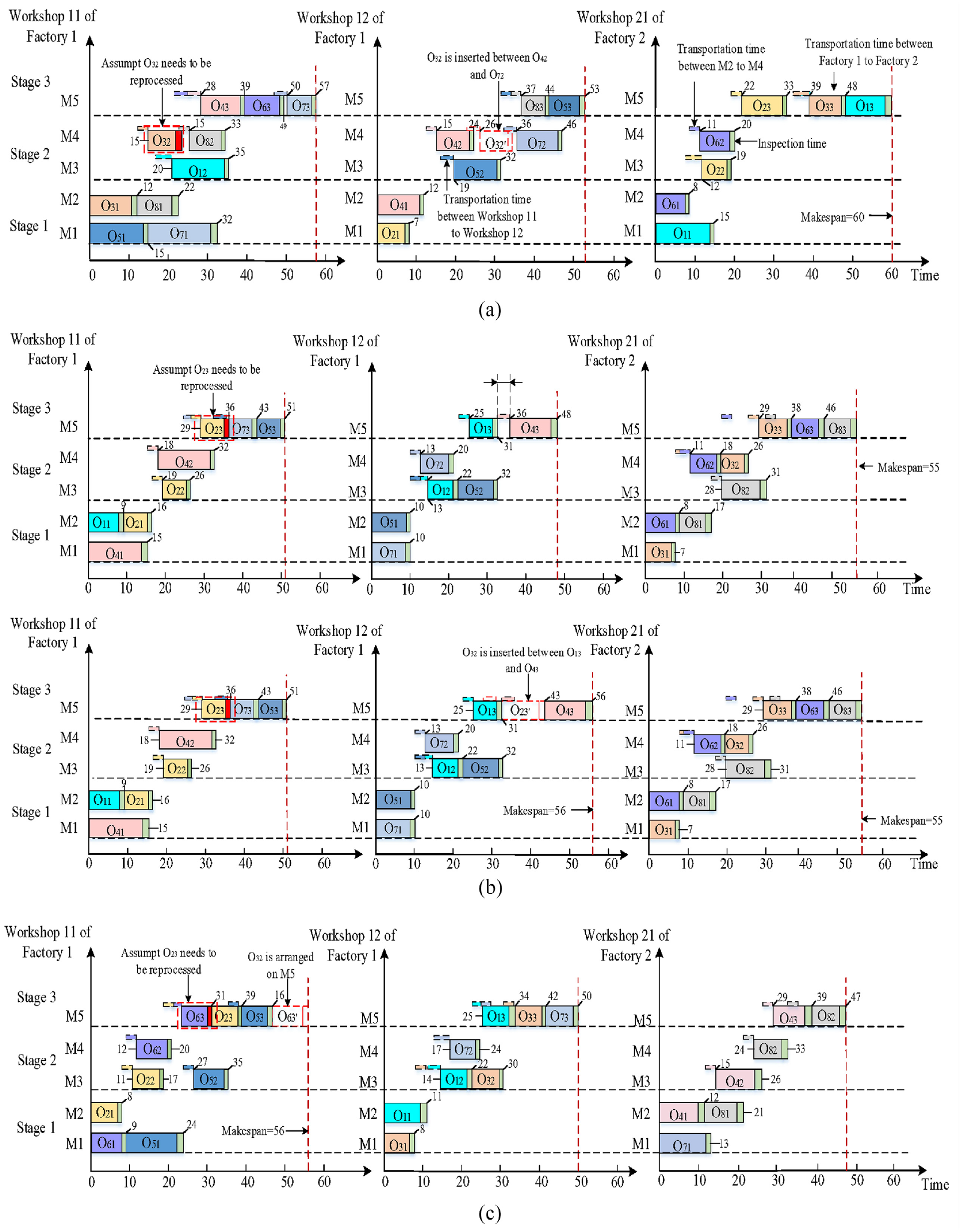
An example of the DRM: (a) strategy 1: assuming O 32 needs to be reprocessed, (b) strategy 2: assuming O 23 needs to be reprocessed, and (c) strategy 3: assuming O 63 needs to be reprocessed.
From Figure 1(a), we can see that O
32
on M4 in workshop 11 of factory 1 needs to be reprocessed (because the color of the square adjacent to O
32
is red), the processing time of O
32
is 7, and the interval time between O
42
and O
72
is 9. Hence, O
32
is inserted into the interval between O
42
and O
72
based on
From Figure 1(b), we can see that O
23
on M5 in workshop 11 of factory 1 needs to be reprocessed (because the color of the square adjacent to O
23
is red), the processing time of O
23
is 6, and the interval time between O
13
and O
43
is 5. Hence, O
23
is inserted into the interval between O
13
and O
43
by moving O
43
to the right based on
From Figure 1(c), we can see that O
63
on M5 in workshop 11 of factory 1 needs to be reprocessed (because the color of the square adjacent to O
63
is red), the processing time of O
63
is 6, and the interval time between each adjacent operation equals to 0. Hence, O
63
is arranged to M5 in workshop 11 of factory 1 (with the smallest cumulative processing time) for reprocessing based on
The proposed IMA
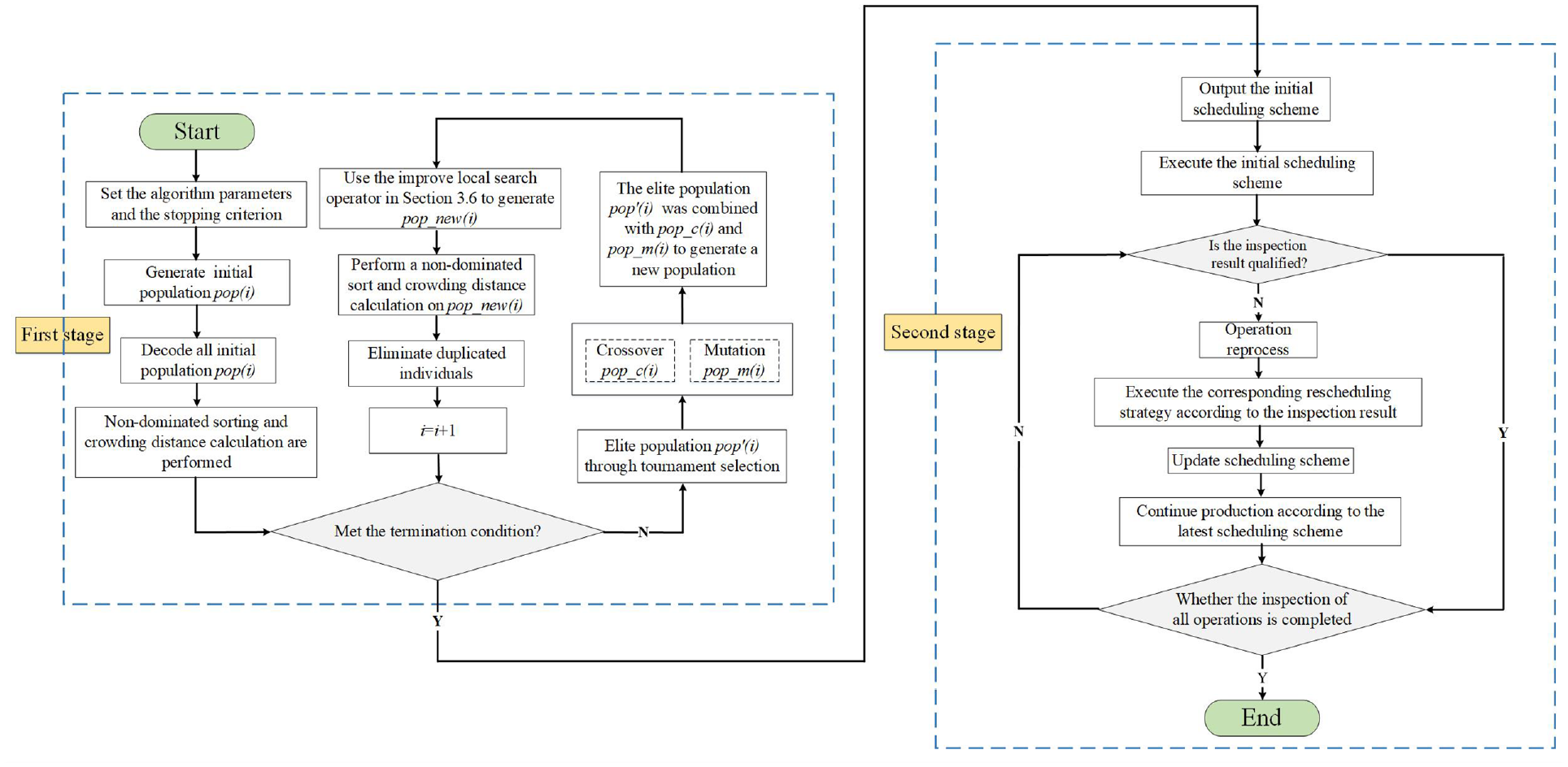
As we all know, the NSGA-II is one of the most popular evolutionary algorithms to solve the production scheduling problems (Deb et al. 68 ), in which a selection strategy is used to choose the excellent individuals for the population, and the non-dominant sorting and crowding distance operators are designed to deal with the optimization objectives. In recent decades, the MA has also been widely used to solve the scheduling problems based on the framework of NSGA-II, in which an efficient local search operator (LSO) is integrated.36,62,63 Here, we propose an IMA to solve the DHFSPR, in which an efficient LSO is combined to expend the solution space and increase the convergence speed while retaining the advantages of both NSGA-II and MA. The framework of the proposed IMA is shown in Figure 2. From Figure 3, we can see that the IMA includes two stages: the initial scheduling stage (marked as “First stage”) and the rescheduling stage (marked as “Second stage”). In the initial scheduling stage, all operations are processed according to the initial scheduling scheme; and in the rescheduling stage, the reprocessing operations and the unfinished operations will be processed according to the rescheduling scheme. The details of the rescheduling method are described in Section 2.6.
The framework of the proposed IMA.
An example of the four-layer encoding method.
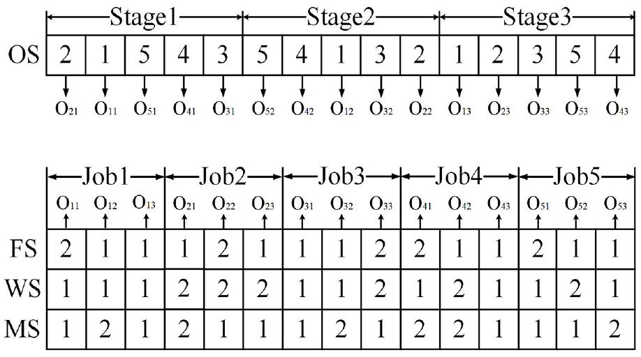
Chromosome encoding
A four-layer encoding method is designed to represent the processing and reprocessing information, which includes the operation sequence vector (OS), inspection result vector (IS), factory sequence vector (FS), workshop sequence vector (WS) and machine sequence vector (MS).
Figure 3 shows an example of this encoding method. Each integer in the OS vector represents the job number, and the number of occurrences of each integer represents the total number of operations for the corresponding job. For example, the second number “2” in stage 2 indicates the second operation of job 2 (O 22 ), which occurs three times, meaning that job 2 has three operations in total. Each integer in the IS vector represents the inspection result of each operation: “0” and “1” mean that the inspection results of the corresponding operations are qualified and unqualified, respectively. Integers in FS, WS, and MS vectors represent the factory, workshop and machine that are assigned to the corresponding operations, respectively. For example, the value [IS, FS, WS, MS] of O 11 is [0, 2, 1, 1], which means that O 11 is processed on machine 1 of workshop 1 in factory 2 and its inspection result is qualified.
Population initialization
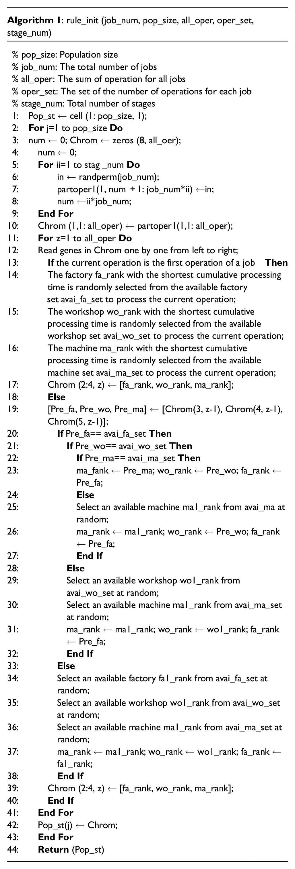
Based on the proposed four-layer encoding operator, a new load balancing initialization method (LBM) for is designed for the IMA to obtain an initial population, aiming at to decrease the transportations among machines, workshops and factories. More specifically, if an operation can be processed on the same machine as its previous operation, it is arranged to be processed at this machine; else if an operation can be processed on another optional machine in the same workshop as its previous operation, it is arranged to be processed at another optional machine in the same workshop; else if an operation can be processed on another optional machine in another workshop of the same factory as its previous operation, it is arranged to be processed at this optional machine in this optional workshop of the same factory; else, the factory, workshop and machine with minimum accumulation processing time are selected. The core pseudocode for initialization is Algorithm 1. The core pseudo code of LBM is shown in Algorithm 1.
Chromosome decoding
In order to process each operation as early as possible and take full use of the advantages of machinable machines, an effective decoding method is employed until all chromosomes are decoded. The specific steps are as follows:

Insert decoding method of the DHFSP: (a) Ta + Tijfwmk + TIij ≤ TE and (b) Ta + Tijfwmk + TIij ≥ TE.
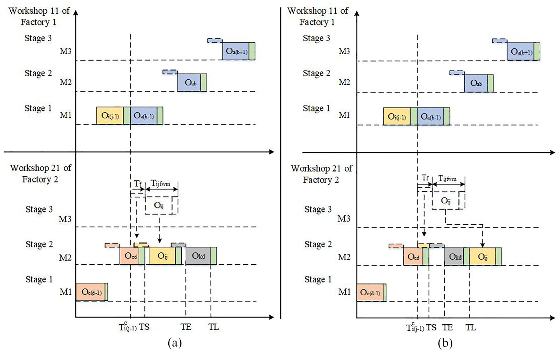
Crossover operator
In the DHFSPR model, in order to avoid infeasible solutions and ensure the diversity of population, a stage crossing method (SCM) is designed in OS vector layer. Figure 5 shows an example of SCM, where P1 and P2 represent the parents and C1 and C2 represent the children. The specific steps of the SCM are as follows:
An illustration of the SCM.
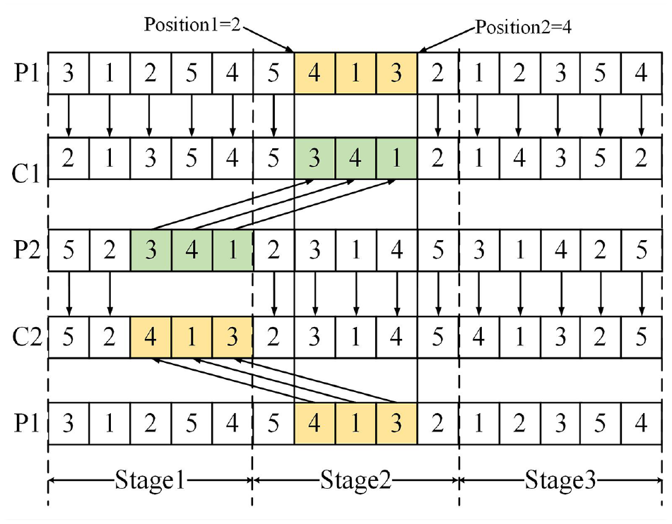
Mutation operators
A two-stage mutation operator (TMO) is proposed for the OS and a random-gene mutation operator (RGM) was designed for FS, WS and MS to expand the solution space while maintaining the diversity of solutions. The specific steps of TMO and RGM are as follows, where P1, P2 represent two parents, and C1, C2 represent two children.
An example of TMO for C1 is shown in Figure 6 as follows:
An illustration of the TMO.
An example of RGM for C2 is shown in Figure 7 as follows:
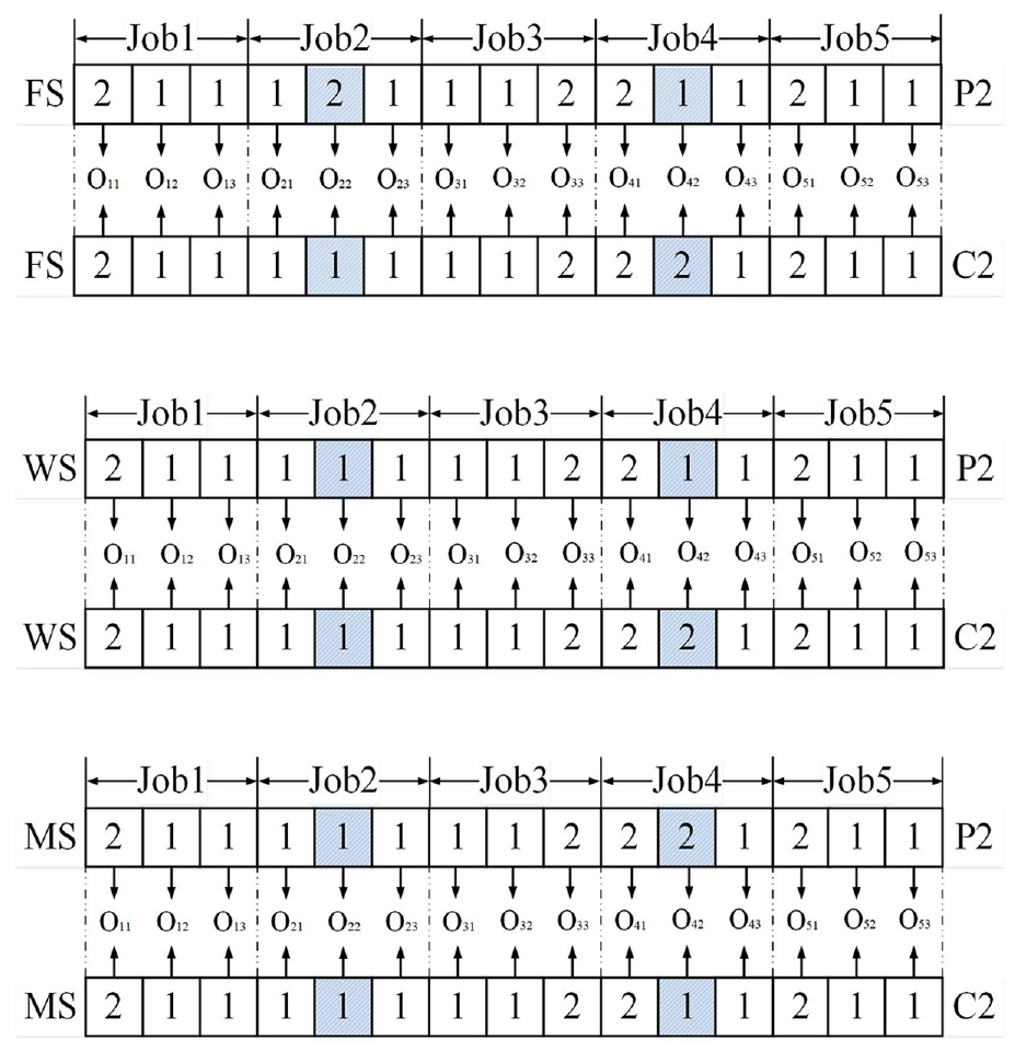
An illustration of the TPM.
The proposed LSO
The LSO have been widely integrated into the evolutionary algorithms to expand the solution space as well as maintain the diversity of the solutions (Asadzadeh, 2015; G. Gong, Chiong, Deng, Han, et al., 2020; G. Gong, Chiong, Deng, & Luo, 2020; X. Gong, Deng, Gong, Liu, & Ren, 2018). Hence, an effective LSO is designed to reduce the maximum completion time by moving critical blocks on the critical path. The proposed LSO includes a position exchange method (PEM) and a machine exchange method (MEM) in the same stage. The probability of PEM and MEM used in the LSO is set to 50%. As shown in Figure 8(a), the critical path is [O 41 ←O 42 ←O 22 ←O 23 ], which contains three critical blocks on different machines.
An example of the proposed LSO: (a) an example of the initial critical path, (b) the result of PEM, and (c) the result of MEM.
An example of PEM is shown in Figure 8(b) as follows:
An example of MEM is shown in Figure 8(c) as follows:
Experiments and analysis
The proposed IMA for the DHFSPR was executed in MATLAB R2018a and run on a computer with an Intel Core i5 2.9 GHz and 16 GB RAM. To test the performance of IMA, a three-part experiment is carried out. Firstly, the key parameters of IMA are determined and compared with other four algorithms. Then, verify the validity of the operators proposed in this paper. Finally, the superior performance of IMA algorithm is proved by comparing with other algorithms. Each benchmark instance was run 10 times to reduce randomness in the experimental results.
Constructing the DHFSPR benchmarks
To test the effectiveness of the proposed IMA in addressing the DHFSP model, 60 new DHFSP benchmark instances (named QHs 01-60) based on some authoritative examples of traditional HFSP standards 61 were built, which can be divided into three sizes: small benchmark instances (QHs 01-20), medium benchmark instances (QHs 21-40), and large benchmark instances (QHs 41-60). In these proposed instances, the number of jobs n = {20,50,100} and the number of stages l = {5,10} constitute an n × l problem scale. Each combination of n and l generates 10 instances, and the processing time is given as a discrete uniform distribution in the interval [1,99]. Randomly generate the same number of factories and workshops for each test problem from [2, 3]. The same number of parallel machines in each stage is uniformly generated within the interval [1, 5], as shown in literature [55], in which at least one stage has two or more parallel machines. In addition, the inspection results of each operation include two types: qualified and unqualified. The operation with qualified inspection result can be directly transported to the next stage for processing, and the operation with unqualified inspection result will be reprocessed by one of its optional machines with shortest processing time. The unqualified rate of each operation is set at 3%.
For all built instances, the processing power of each machine is set to a random number of 10–20; the unit inspection time of each operation is set as a random number between 10 and 18; unit transportation time between two different factories, workshops and machines is set at 80, 40 and 20, respectively; and the operation transportation and processing power are set to 10. The constructed instances QHs 01-60 can be downloaded from: https://github.com/QiYanzu/DHFSP.
Performance metrics
To test the performance of different algorithms, there are three widely used and effective performance evaluation methods, including: the Set Coverage indicator (C-metric), 64 Inverted Generational Distance (IGD), 65 and Hypervolume indicator (HV). 66 For the SC, the larger the value of C (A, B), the better the solution set of A, and vice versa; for the IGD, the lower the IGD value, the better the algorithm performance, and vice versa; and for the HV, the higher the HV value, the better the algorithm performance, and vice versa. More specific descriptions can be seen from the corresponding references.
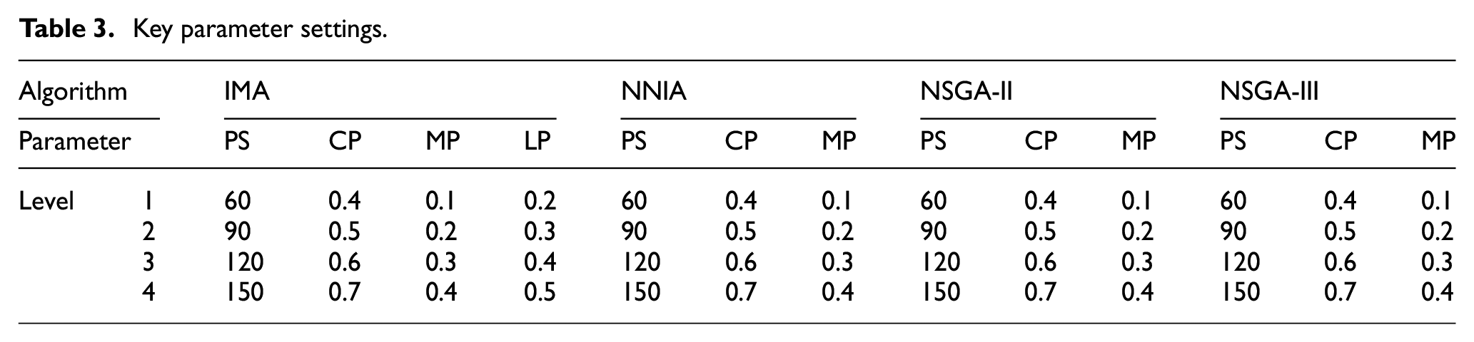
Parameter settings
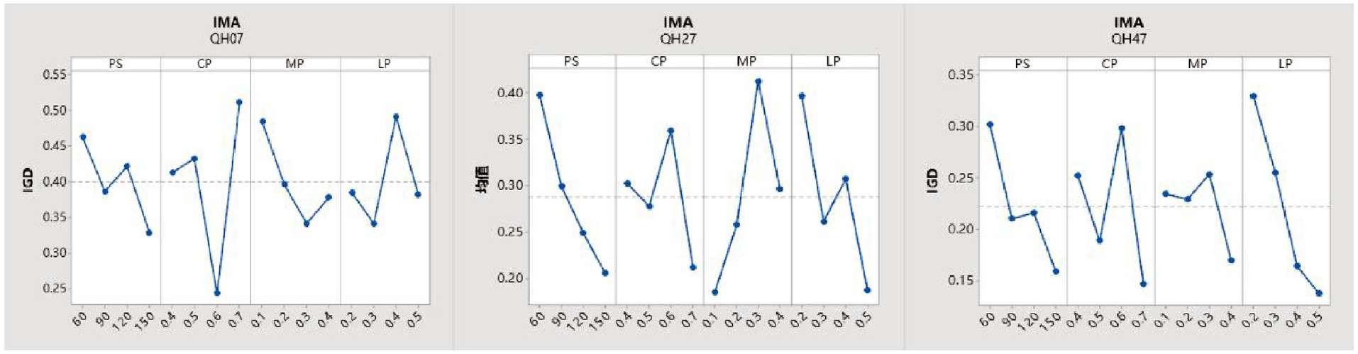
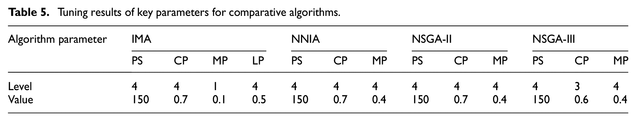
Different parameters will affect the overall performance of the algorithm, so we need to adjust the key parameters of the compared algorithms. In this paper, the Taguchi experimental design method 31 was used to determine the optimal parameter values of each algorithm (IMA, NNIA, NSGA-II, NSGA-III). Four levels setting of each key parameter are shown in Table 3. There are four key parameters: the population size (PS), crossover probability (CP), mutation probability (MP) and LSO probability (LP). Three instances are selected for the experiment including small-scale (QH 07), medium-scale (QH 27) and large-scale (QH 47), and the IGD is selected as the evaluation index for the experimental results.
Key parameter settings.
Parameters calibration of IMA
According to the Taguchi experimental method, an orthogonal table is used to set the parameter combinations of the experiments (the details can refer to the Montgomery 31 ). In short, in the orthogonal table, the total number of occurrences of each level in each column (representing each factor) is equal; and the level combination of different rows in any two columns is different. Hence, based on the parameter settings in Table 3, we can obtain an orthogonal table with 16 degrees of freedom. As shown in Table 4, a total of 16 parameter combinations are shown in columns 2–5 and the IGD value of parameter combinations are shown in columns 6–8.
Orthogonal allay and results.
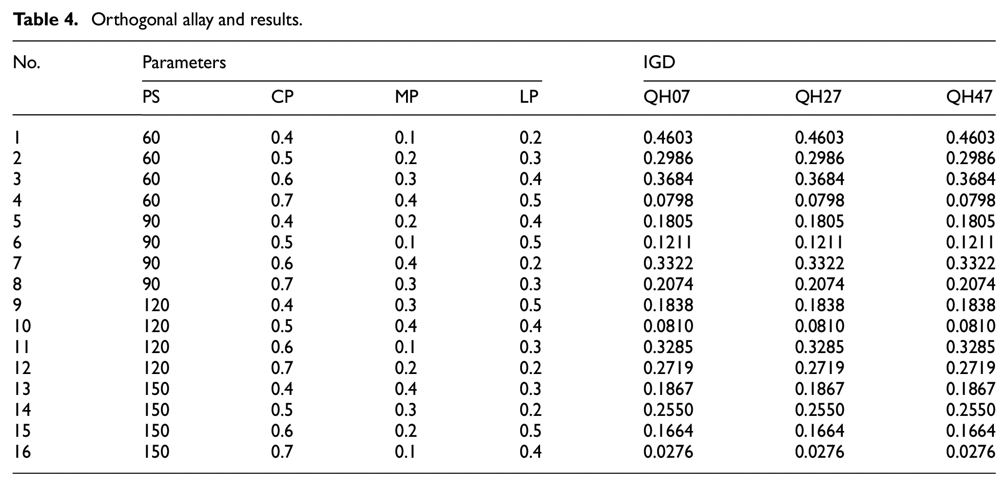
Based on the results in Table 4, the rank changes of IMA parameters are shown in Figure 9. For the PS, the minimum value of IGD is found at the first level for QH 01, QH 27, and QH 47; hence, the PS is set as 150. For the CP, the minimum value of IGD is found at the fourth level for QH 27 and QH 47, and the minimum value of IGD is found at the first level for QH 07, hence, the CP is set as 0.7. For the MP, the minimum value of IGD is found at the third, first and fourth levels respectively, for QH 01, QH 27, and QH 47, but the first level of Q27 is the lowest, hence, the MP is set as 0.1. For the LP, the minimum value of IGD is found at the fourth level for QH 27 and QH 47 and at the second level for QH 07, hence, the LP is set as 0.5.
Main effect of key parameter of IMA.
Based on the above result analysis, the optimal key parameters of the IMA are set as follows: PS = 150, CP = 0.7, MP = 0.1, and LP = 0.5 (see Table 5).
Tuning results of key parameters for comparative algorithms.
Parameters calibration of the comparison algorithms
In this paper, NNIA, 67 NSGA-II, 68 and NSGA-III 69 are selected as comparison algorithms. The main reasons for choosing these three comparison algorithms are as follows: (1) all of the NNIA, NSGA-II, NSGA-III, and IMA are based on traditional genetic algorithms, so they have similar frameworks; (2) all these algorithms use the non-dominated sorting method to deal with multi-objective problems; and (3) all these algorithms are classical algorithms are usually used as the baseline algorithms to verify the effectiveness of the newly proposed multi-objective algorithms.
To ensure the fairness of the experiment, the Taguchi experiment is also used to calibrate the key parameters of the NNIA, NSGA-II and NSGA-III based on three instances (QH 07, QH 27, and QH 47). The key parameters and level settings of each algorithm are shown in Table 3. The variation trend of each parameter level of the three comparison algorithms is plotted in Figure A1. As shown in Table 5, the key parameter combinations of NNIA, NSGA-II, and NSGA-III were obtained using the same analytical method as IMA.
Evaluate the effectiveness of the proposed LSO
In order to verify the effectiveness of the LSO in the algorithm IMA, we compared the results of IMA with LSO and IMA without LSO (IMA1). A total of 40 instances (including large, medium, and small size) were solved by IMA and IMA1, and evaluated their performance against C-metric, IGD and HV. Each experiment is performed independently 10 times.
The experimental results of IMA and IMA1 are shown in Table A1 of the Appendix. It can be seen from the experimental results that the performance of IMA is obviously better than that of IMA1. Therefore, it is proved that LSO expands the solution space in the search process, improves the convergence speed of the algorithm, and enables the algorithm to obtain better solutions.
Comparison of rescheduling methods
According to the survey, there is no literature on the dynamic scheduling of operational reprocessing, so there is no suitable strategy for comparison. However, right-shift rescheduled strategy is often used to deal with dynamic scheduling problems in other scheduling problems.70–75 Hence, in order to verify the effectiveness of the DRM to handle the remaining operations after operations reprocessing, the results obtained by using IMA with the DRM(IMA2) will be compared with those by using IMA with the right-shift rescheduled method (RRS) (IMA3). The RRS method is described as follows: after the results of the operation inspection are confirmed, each rescheduling operation is immediately scheduled to the original machine for reprocessing, and the affected operations are moved to the right accordingly.
In the experiment, a total of 40 instances (QHs 01-05, QHs 11-15, QHs 21-25, QHs 31-45, QHs 51-60) are selected, and each instance is run independently 10 times (the termination criterion was set to 100 iterations).
Based on C-metric, IGD, and HV, the final evaluation results of the IMA2 and IMA3 are shown in Table A2 of the Appendix. From the table, it can be clearly seen from the C-metric value that IMA2 is better than IMA3 in all instances; from the IGD value, it is clear that IMA2 has an overwhelming advantage over IMA3 in all instances, except for QH 11; and from the HV value, it is clear that IMA2 is better than IMA3 in all instances. Hence, based on the above results and analysis, the solution obtained by IMA2 is significantly better than that obtained by IMA3, which proves that the proposed DRM has superior performance in handling operation reprocessing.
Comparison with other algorithms
To further verify the performance of the proposed IMA algorithm, it is compared with three well-known multi-objective algorithms, namely NNIA, NSGA-II, and NSGA-III. For the fairness of the experiment, NNIA, NSGA-II, and NSGA-III used the same initialization method, crossover and mutation operators as our proposed IMA in 60 benchmark instances. The key parameters of all comparison algorithms were calibrated in Section 4.3, and the operating conditions and stopping criteria of the comparison algorithms were consistent with IMA.
To ensure the fairness and rationality of the experiment, we divided the experimental process into two parts. The first part takes 100 iterations as the stopping criterion, and each algorithm runs independently 10 times; and the second part takes the minimum average running time form the first stage for each instance, and each algorithm also runs independently 10 times.
In the first part, the comparison results based on C-metric, HV and IGD are recorded in Tables A3 and A4 of the Appendix. As can be seen from Table A3, based on C-metric, it can be seen that the proposed IMA outperforms the NNIA on most of the instances except QH 10, QH 12, and QH 31; outperforms the NSGA-II and NSGA-III on all instances. As can be seen from Table A4, based on IGD, 89%, 98%, and 98% of the instances solved by IMA are better than NNIA, NSGA-II, and NSGA-III, respectively; and based on HV, 92%, 98%, and 98% of the instances solved by IMA are better than NNIA, NSGA-II, and NSGA-III, respectively.
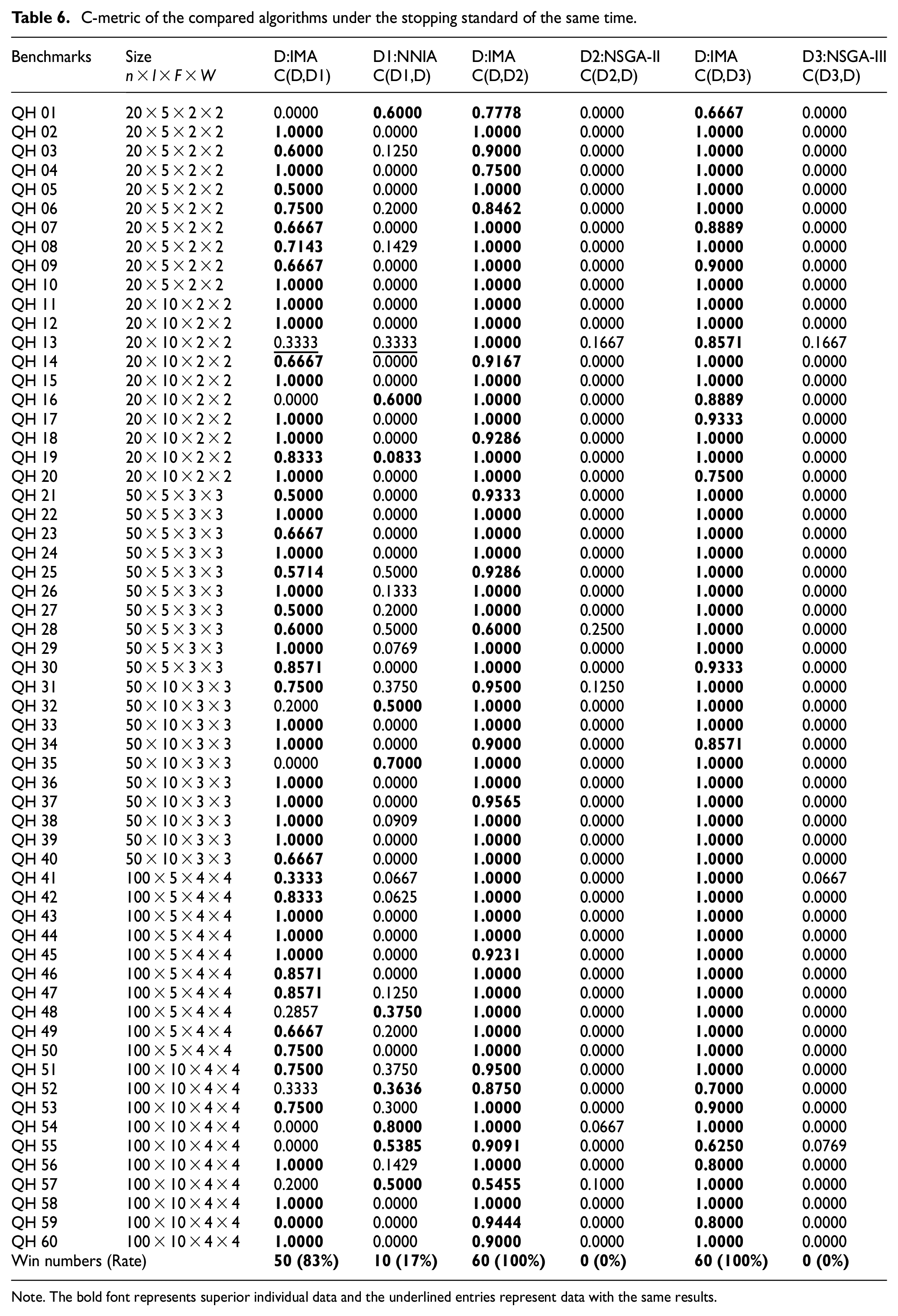
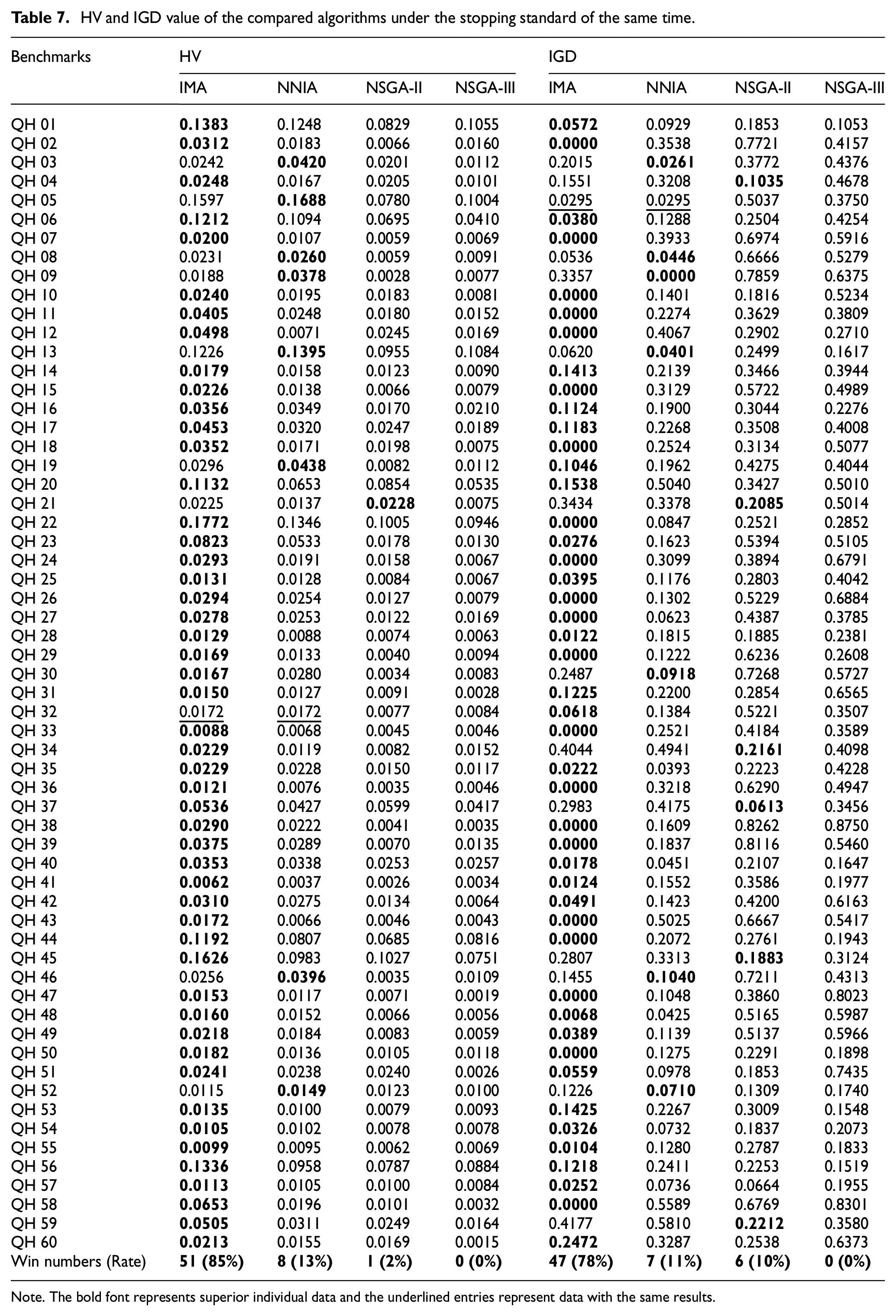
In the second part, the rescheduling scheme comparison results generated by four comparison algorithms based on C-metric, IGD and HV are shown in Tables 6 and 7. As can be seen from Table 6, based on the C-metric, 83%, 100%, and 100% of the instances solved by IMA were better than NNIA, NSGA-II, and NSGA-III, respectively. It can be seen from Table 7, 87%, 98%, and 100% of the instances solved by IMA based on HV are better than NNIA, NSGA-II, and NSGA-III, respectively; and based on IGD, IMA solved 89%, 90%, and 100% of the instances better than NNIA, NSGA-II, and NSGA-III, respectively.
C-metric of the compared algorithms under the stopping standard of the same time.
Note. The bold font represents superior individual data and the underlined entries represent data with the same results.
HV and IGD value of the compared algorithms under the stopping standard of the same time.
Note. The bold font represents superior individual data and the underlined entries represent data with the same results.
Therefore, based on the experimental results of the above two parts, it can be concluded that the IMA proposed in this paper is significantly better than the comparison algorithm in terms of convergence, distribution, and quality of non-dominated solutions under the same number of iterations and the same running time, which confirms the high performance of IMA algorithm in solving DHFSP.
To better demonstrate the performance of IMA, Figure 10 display the mean plots of SC, IGD, and HV for four algorithms with 95% CI (confidence interval, CI), from which we can observe that the significant difference among the four algorithms. Based on the figure, the C-metric interval range of IMA is closer to 1 than that of NNIA, NSGA-III, and NSGA-II, hence IMA is superior to NNIA, NSGA-III, and NSGA-II. The overall performance order of the four algorithms for solving the scheduling scheme is as follows: IMA > NNIA > NSGA-II > NSGA-III. At the same time, Table 8 records the non-parametric statistical test of Wilcoxon’s signed rank test at 95% confidence level, indicating significant differences between IMA and the comparison algorithms, because the p-values are far less than 0.05.
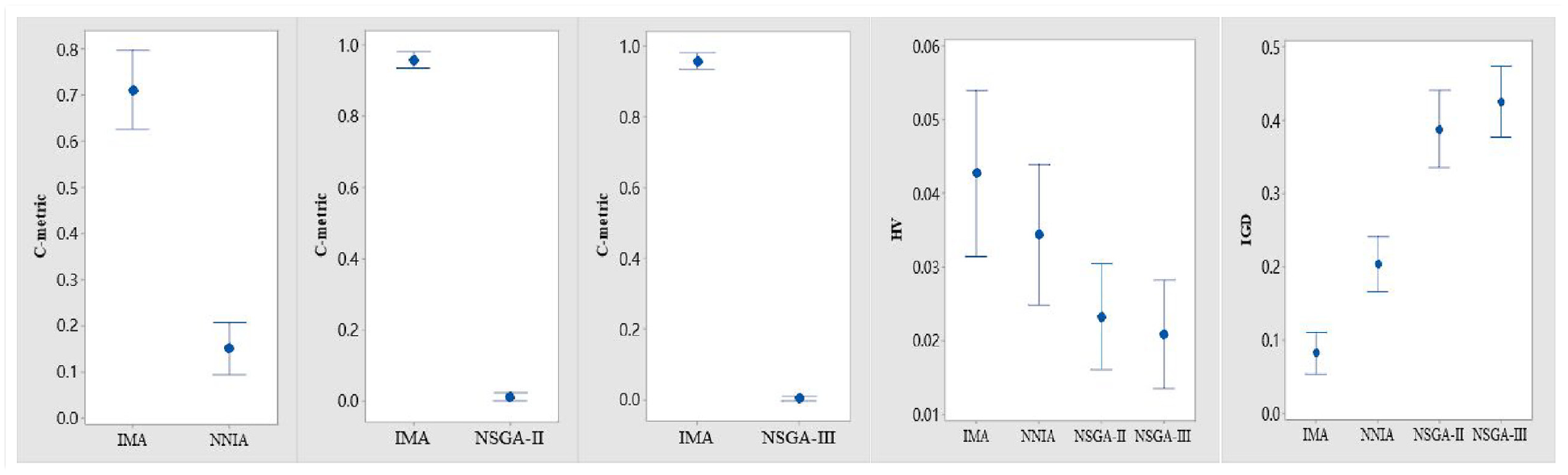
Mean plots with 95% CI in terms of C-metric, HV and IGD results of four algorithms.
Wilcoxon signed-rank test.
In order to visually display the distribution of non-dominated solutions of the algorithm, nine instances (QH 07, QH 12, QH 22, QH 26, QH 30, QH 35, QH 41, QH 47, QH 58) are randomly selected and their Pareto front (PF) distributions were drawn in Figure 11. It can be seen from Figure 11(a) to (i) that the PFs distribution of IMA is closer to the bottom of the graph, indicating that the solution obtained by IMA has a higher probability to dominate the solutions obtained by other three algorithms.
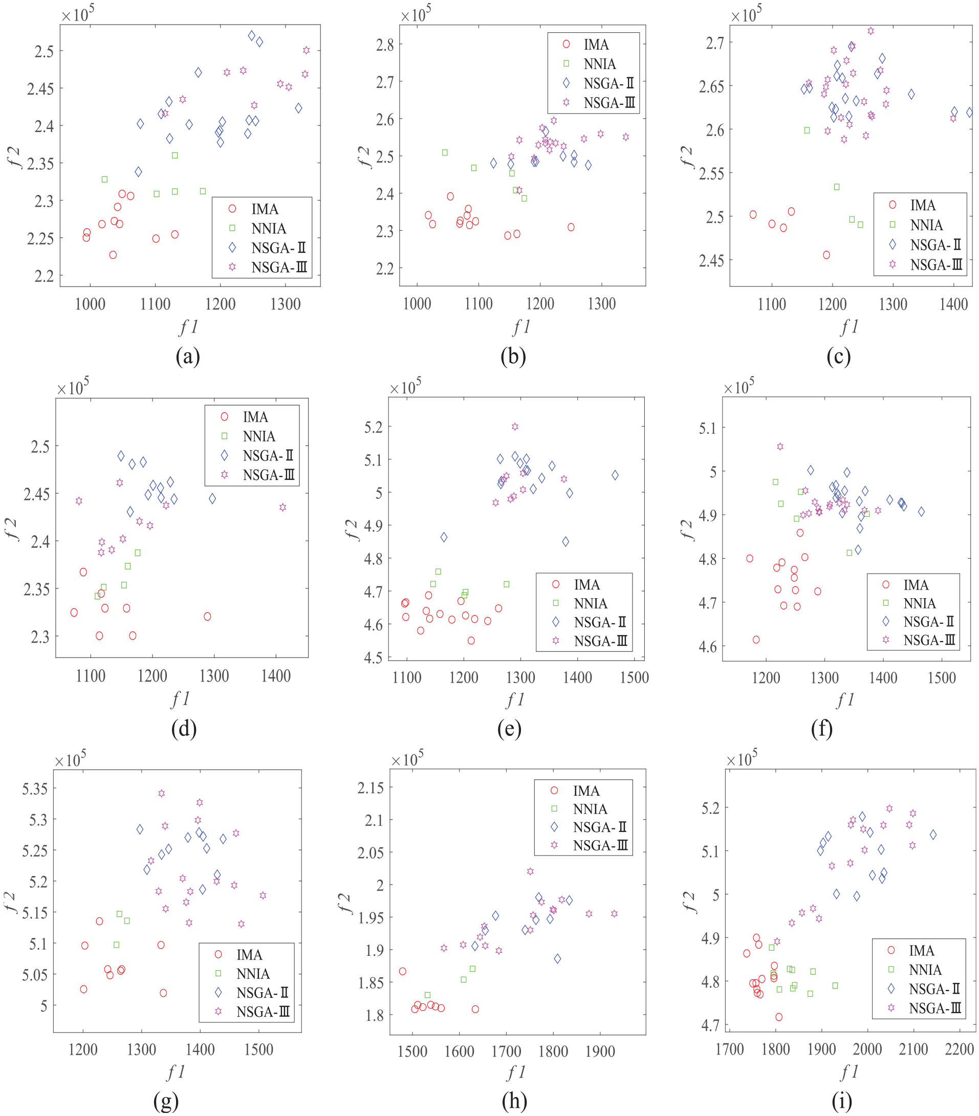
PF results of selected instances: (a) QH 07, (b) QH 12, (c) QH 22, (d) QH 26, (e) QH 30, (f) QH 35, (g) QH 41, (h) QH 47, and (i) QH 58.
Figures 12 and 13 show two Gantt charts of the initial scheduling scheme and rescheduling scheme generated by IMA for QH01. It can be seen from Figure 13 that all operations are inspected after processing, and O 31 , O 42 , and O 122 are required to be reprocessed according to the inspection results. The inspection results and rescheduling process are as follows:
The first operation O
31
of job 3 and the second operation O
42
of job 4 need to be reprocessed (the inspection results of O
31
and O
42
in Figure 13 are marked in red). According to
The second operation O
122
of job 12 also need to be reprocessed. According to
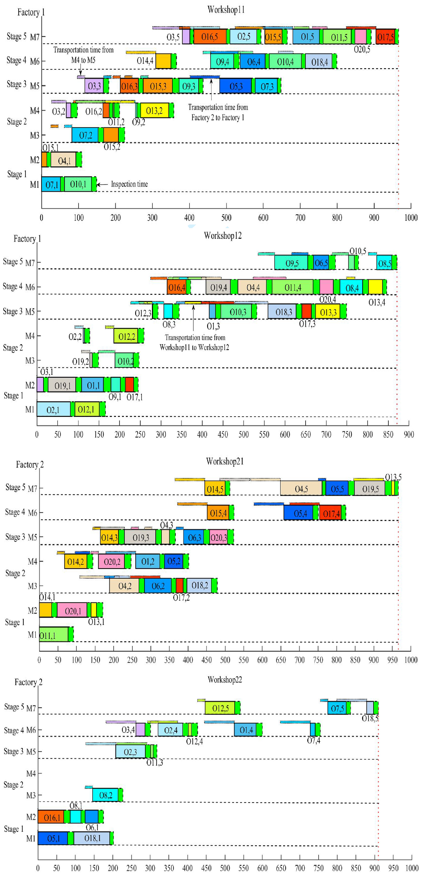
An initial scheduling scheme of QH 01 with IMA before rescheduling.
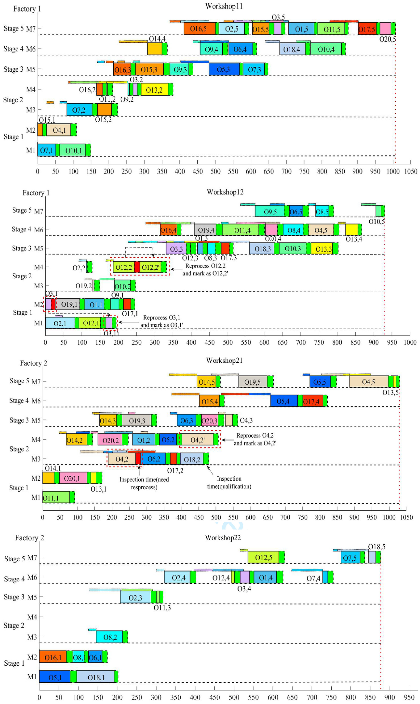
A rescheduling scheme of QH 01 with IMA after rescheduling.
The check results of all other job operations are qualified (the test results are marked in green in Figure 13), that is, keep the latest scheduling scheme unchanged and continue to process the unprocessed operations of other jobs.
Conclusions
In this paper, we have presented a new model of DHFSPR – distributed hybrid flow shop scheduling with operation inspection and reprocessing. This model is the first to consider operation inspection and reprocessing in the context of distributed hybrid flow shop scheduling. We proposed an IMA algorithm to solve the DHFSPR aiming at minimizing the makespan and total energy consumption simultaneously. In the IMA, a four-layer encoding method and a new load balanced initialization method were proposed to expand the solution space while maintaining the diversity of the population; a random stage crossover operator and a two-stage mutation operator were designed to expand the search space of the solutions; an LSO containing two methods was proposed to improve the local search ability and convergence speed of the IMA; and a DRM was designed to deal with the unqualified operations.
In the experimental part, we first constructed 60 benchmark instances based on some HFSP classic benchmark instance to test the performance of the algorithm. To be fair, the key parameters of IMA and other three compared algorithms (NNIA, NSGA-II and NSGA-III) were calibrated by using the Taguchi method. In addition, 40 large, medium and small cases were selected to verify the effectiveness of the proposed LSO and DRM. Furthermore, extensive comparisons were carried out between our proposed IMA and three well-known algorithms based on the 60 constructed benchmark instances. From these experimental results, we can see that the IMA is significantly better than other three compared algorithms based on the C-metric, IGD and HV evaluation indexes.
Our work has both theoretical and practical contributions. In theory, we have pioneered a new research direction of the DHFSP, which considers the real production factors of operational inspection and reprocessing for the first time. From the perspective of practical application, the DHFSPR model can help production managers to deal with unqualified operations, avoiding unreasonable material distribution and unnecessary waste of production resources, so that to improve productivity and resource utilization.
In the future, we will study the DHFSPR in more detail. For example, the changes of delivery times and inventory capacity, and the shortages of raw materials may be taken into consideration.
Footnotes
Appendix
IGD and HV value of the compared algorithms under the stopping standard of 100 iterations.
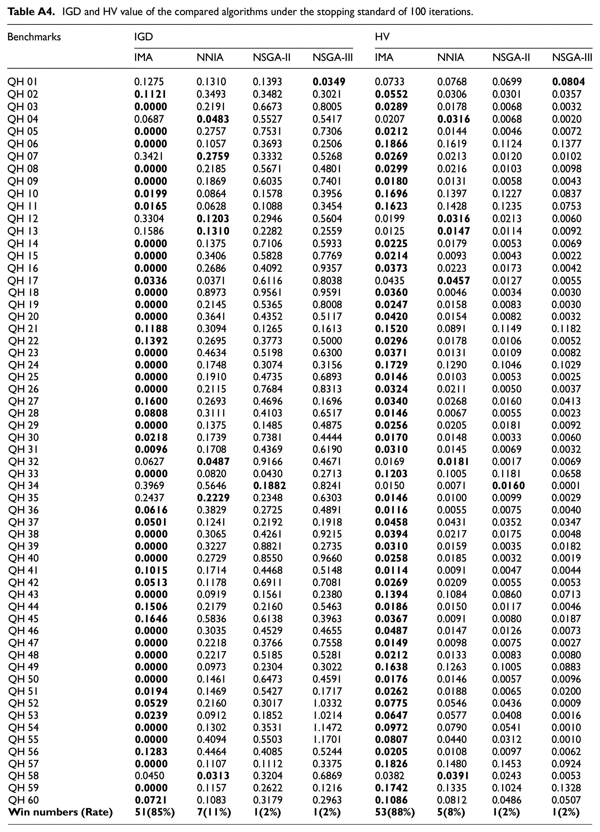
| Benchmarks | IGD | HV | ||||||
|---|---|---|---|---|---|---|---|---|
| IMA | NNIA | NSGA-II | NSGA-III | IMA | NNIA | NSGA-II | NSGA-III | |
| QH 01 | 0.1275 | 0.1310 | 0.1393 |
|
0.0733 | 0.0768 | 0.0699 |
|
| QH 02 |
|
0.3493 | 0.3482 | 0.3021 |
|
0.0306 | 0.0301 | 0.0357 |
| QH 03 |
|
0.2191 | 0.6673 | 0.8005 |
|
0.0178 | 0.0068 | 0.0032 |
| QH 04 | 0.0687 |
|
0.5527 | 0.5417 | 0.0207 |
|
0.0068 | 0.0020 |
| QH 05 |
|
0.2757 | 0.7531 | 0.7306 |
|
0.0144 | 0.0046 | 0.0072 |
| QH 06 |
|
0.1057 | 0.3693 | 0.2506 |
|
0.1619 | 0.1124 | 0.1377 |
| QH 07 | 0.3421 |
|
0.3332 | 0.5268 |
|
0.0213 | 0.0120 | 0.0102 |
| QH 08 |
|
0.2185 | 0.5671 | 0.4801 |
|
0.0216 | 0.0103 | 0.0098 |
| QH 09 |
|
0.1869 | 0.6035 | 0.7401 |
|
0.0131 | 0.0058 | 0.0043 |
| QH 10 |
|
0.0864 | 0.1578 | 0.3956 |
|
0.1397 | 0.1227 | 0.0837 |
| QH 11 |
|
0.0628 | 0.1088 | 0.3454 |
|
0.1428 | 0.1235 | 0.0753 |
| QH 12 | 0.3304 |
|
0.2946 | 0.5604 | 0.0199 |
|
0.0213 | 0.0060 |
| QH 13 | 0.1586 |
|
0.2282 | 0.2559 | 0.0125 |
|
0.0114 | 0.0092 |
| QH 14 |
|
0.1375 | 0.7106 | 0.5933 |
|
0.0179 | 0.0053 | 0.0069 |
| QH 15 |
|
0.3406 | 0.5828 | 0.7769 |
|
0.0093 | 0.0043 | 0.0022 |
| QH 16 |
|
0.2686 | 0.4092 | 0.9357 |
|
0.0223 | 0.0173 | 0.0042 |
| QH 17 |
|
0.0371 | 0.6116 | 0.8038 | 0.0435 |
|
0.0127 | 0.0055 |
| QH 18 |
|
0.8973 | 0.9561 | 0.9591 |
|
0.0046 | 0.0034 | 0.0030 |
| QH 19 |
|
0.2145 | 0.5365 | 0.8008 |
|
0.0158 | 0.0083 | 0.0030 |
| QH 20 |
|
0.3641 | 0.4352 | 0.5117 |
|
0.0154 | 0.0082 | 0.0032 |
| QH 21 |
|
0.3094 | 0.1265 | 0.1613 |
|
0.0891 | 0.1149 | 0.1182 |
| QH 22 |
|
0.2695 | 0.3773 | 0.5000 |
|
0.0178 | 0.0106 | 0.0052 |
| QH 23 |
|
0.4634 | 0.5198 | 0.6300 |
|
0.0131 | 0.0109 | 0.0082 |
| QH 24 |
|
0.1748 | 0.3074 | 0.3156 |
|
0.1290 | 0.1046 | 0.1029 |
| QH 25 |
|
0.1910 | 0.4735 | 0.6893 |
|
0.0103 | 0.0053 | 0.0025 |
| QH 26 |
|
0.2115 | 0.7684 | 0.8313 |
|
0.0211 | 0.0050 | 0.0037 |
| QH 27 |
|
0.2693 | 0.4696 | 0.1696 |
|
0.0268 | 0.0160 | 0.0413 |
| QH 28 |
|
0.3111 | 0.4103 | 0.6517 |
|
0.0067 | 0.0055 | 0.0023 |
| QH 29 |
|
0.1375 | 0.1485 | 0.4875 |
|
0.0205 | 0.0181 | 0.0092 |
| QH 30 |
|
0.1739 | 0.7381 | 0.4444 |
|
0.0148 | 0.0033 | 0.0060 |
| QH 31 |
|
0.1708 | 0.4369 | 0.6190 |
|
0.0145 | 0.0069 | 0.0032 |
| QH 32 | 0.0627 |
|
0.9166 | 0.4671 | 0.0169 |
|
0.0017 | 0.0069 |
| QH 33 |
|
0.0820 | 0.0430 | 0.2713 |
|
0.1005 | 0.1181 | 0.0658 |
| QH 34 | 0.3969 | 0.5646 |
|
0.8241 | 0.0150 | 0.0071 |
|
0.0001 |
| QH 35 | 0.2437 |
|
0.2348 | 0.6303 |
|
0.0100 | 0.0099 | 0.0029 |
| QH 36 |
|
0.3829 | 0.2725 | 0.4891 |
|
0.0055 | 0.0075 | 0.0040 |
| QH 37 |
|
0.1241 | 0.2192 | 0.1918 |
|
0.0431 | 0.0352 | 0.0347 |
| QH 38 |
|
0.3065 | 0.4261 | 0.9215 |
|
0.0217 | 0.0175 | 0.0048 |
| QH 39 |
|
0.3227 | 0.8821 | 0.2735 |
|
0.0159 | 0.0035 | 0.0182 |
| QH 40 |
|
0.2729 | 0.8550 | 0.9660 |
|
0.0185 | 0.0032 | 0.0019 |
| QH 41 |
|
0.1714 | 0.4468 | 0.5148 |
|
0.0091 | 0.0047 | 0.0044 |
| QH 42 |
|
0.1178 | 0.6911 | 0.7081 |
|
0.0209 | 0.0055 | 0.0053 |
| QH 43 |
|
0.0919 | 0.1561 | 0.2380 |
|
0.1084 | 0.0860 | 0.0713 |
| QH 44 |
|
0.2179 | 0.2160 | 0.5463 |
|
0.0150 | 0.0117 | 0.0046 |
| QH 45 |
|
0.5836 | 0.6138 | 0.3963 |
|
0.0091 | 0.0080 | 0.0187 |
| QH 46 |
|
0.3035 | 0.4529 | 0.4655 |
|
0.0147 | 0.0126 | 0.0073 |
| QH 47 |
|
0.2218 | 0.3766 | 0.7558 |
|
0.0098 | 0.0075 | 0.0027 |
| QH 48 |
|
0.2217 | 0.5185 | 0.5281 |
|
0.0133 | 0.0083 | 0.0080 |
| QH 49 |
|
0.0973 | 0.2304 | 0.3022 |
|
0.1263 | 0.1005 | 0.0883 |
| QH 50 |
|
0.1461 | 0.6473 | 0.4591 |
|
0.0146 | 0.0057 | 0.0096 |
| QH 51 |
|
0.1469 | 0.5427 | 0.1717 |
|
0.0188 | 0.0065 | 0.0200 |
| QH 52 |
|
0.2160 | 0.3017 | 1.0332 |
|
0.0546 | 0.0436 | 0.0009 |
| QH 53 |
|
0.0912 | 0.1852 | 1.0214 |
|
0.0577 | 0.0408 | 0.0016 |
| QH 54 |
|
0.1302 | 0.3531 | 1.1472 |
|
0.0790 | 0.0541 | 0.0010 |
| QH 55 |
|
0.4094 | 0.5503 | 1.1701 |
|
0.0440 | 0.0312 | 0.0010 |
| QH 56 |
|
0.4464 | 0.4085 | 0.5244 |
|
0.0108 | 0.0097 | 0.0062 |
| QH 57 |
|
0.1107 | 0.1112 | 0.3375 |
|
0.1480 | 0.1453 | 0.0924 |
| QH 58 | 0.0450 |
|
0.3204 | 0.6869 | 0.0382 |
|
0.0243 | 0.0053 |
| QH 59 |
|
0.1157 | 0.2622 | 0.1216 |
|
0.1335 | 0.1024 | 0.1328 |
| QH 60 |
|
0.1083 | 0.3179 | 0.2963 |
|
0.0812 | 0.0486 | 0.0507 |
|
|
|
|
|
|
|
|
|
|
Declaration of conflicting interests
The author(s) declared no potential conflicts of interest with respect to the research, authorship, and/or publication of this article.
Funding
The author(s) disclosed receipt of the following financial support for the research, authorship, and/or publication of this article: This work was supported by the National Nature Science Foundation of China (grant number: 72001217); the Nature Science Foundation of Hunan (grant number: 2021JJ41081; 2022JJ40860); the Hunan Provincial Department of Education Project (grant number: 22A0170); the Changsha Soft Science Research Program (grant number: kh2302004); and the Hunan Provincial Innovation Foundation for Postgraduate (grant number: CX20220736).
Data availability statement
Data sharing not applicable to this article as no datasets were generated or analyzed during the current study.