Sage Journals: Discover world-class research

Abstract

Aiming at the problem that it takes a long time and high cost to obtain complete labeled data under intelligent fault diagnosis and unlabeled data is not used. This paper proposes an improved semi-supervised mean teacher deep learning (MTDL) and Gramian angle field (GAF) fusion diagnostic method. This method fully utilizes a small number of labeled samples and a large number of unlabeled samples to deeply mine invisible fault features and potential physical correlations. At the same time, it solves the problem of losing the inter-data correlation structure when one-dimensional time series signals are used as inputs for neural networks. The GAF-MTDL method uses consistency regularization and modifies the network structure in the mean teacher algorithm into a semi-supervised deep learning model enhanced by WideResNet. The experimental results show that the proposed GAF-MTDL method saves a lot of manual labeling costs, improves the recognition accuracy and generalization ability, and can achieve excellent prediction accuracy with very little labeled data. In the end, the accuracy of planetary gear fault identification reached 98.22% under the labeling rate of 20%, and the accuracy of fault identification reached 99.98% through the verification of the bearing data set of Case Western Reserve University. The value of this research is to bring an efficient and low-cost technology to the field of industrial intelligent fault diagnosis, which can significantly improve the accuracy of fault identification.

Keywords

GAF image encoding gearbox fault diagnosis semi-supervised deep learning WideResNet

Introduction

Gearbox is a commonly used power transmission equipment in rotating machinery. As an important component, it has been widely used in vehicle transmission, aerospace, robotics, manufacturing equipment, etc.¹ Gearboxes usually have to withstand complex and harsh operating conditions, such as high temperature, high humidity, high load, high speed, etc. These factors increase the occurrence of failures to varying degrees, causing adverse effects on the economy and even casualties.^2,3 Therefore, the condition monitoring and fault diagnosis of the gearbox are very important to ensure the reliability and safety of the system.

Deep learning-based methods are increasingly popular in the field of mechanical fault diagnosis.^4–7 Since deep learning can adaptively adjust model parameters according to different characteristics of the input data, it does not require manual operation and rich expert experience. It only requires the powerful nonlinear extraction ability of the network itself to improve the adaptability to different data sets. The ability to extract, start learning from the most original data, and automatically mine the potential features of the data, so as to obtain high fault diagnosis accuracy.

For example, convolutional neural network (CNN)⁸ is an image recognition method for identifying faults in rotating machinery. CNN has stronger applicability and can learn effective data features. Many scholars use it for rotating machinery fault diagnosi.⁹ Feng et al.¹⁰ proposed a spur gear wear monitoring framework based on cyclostationarity in an intelligent manufacturing system, using the squared envelope (SE) of the residual signal to remove the deterministic component to identify gear wear distribution and its propagation trend. The established framework based on cyclic stability accurately manages the health of the gear transmission system. Zhang et al.¹¹ propose a neural network approach that combines multiple attention mechanisms. The method processes the signal data, pays attention to the frequency band where the significant features of the wavelet coefficients are located, realizes the enhancement of the model, and greatly improves the recognition ability. In addition, this fault diagnosis method effectively improves the sensitivity of the convolutional neural network. Zhang et al.¹² proposed a fault diagnosis method for convolutional neural networks based on data probability density. The 1D data is converted into 2D data with obvious features, and the convolutional neural network selects LeNet-5 to improve the fault diagnosis accuracy. Feng et al.¹³ proposed a Vold-Kalman filter bandwidth selection scheme based on order spectrum for gearbox fault diagnosis of offshore wind turbines. The time waveform of short transient harmonics can be extracted and tracked without phase offset, which is very beneficial to the status monitoring of offshore wind turbines. Feng et al.¹⁴ proposed a digital twin-driven intelligent health management method that can accurately evaluate the gear wear process. At the same time, a transfer learning algorithm is used to transfer knowledge from the digital twin model and apply the learned knowledge to evaluate the surface wear of the physical structure. The above methods are all supervised learning models, which require manual operation during fault diagnosis. In reality, obtaining labels for large amounts of data requires a lot of costs.

Supervised learning requires manual labeling of a large number of samples in practical applications,¹⁵ while unsupervised learning^16,17 often has lower accuracy and no labeled data and directional information features, which may cause task failure. Semi-supervised learning is an integrated improvement of unsupervised and supervised learning, which neither wastes unlabeled data but also trains with labeled data. As the training learning content increases, the output model obtained becomes more stable.¹⁸ Zaman and Liang¹⁹ proposed an image-based semi-supervised fault diagnosis method. The core idea is to use a small number of labeled images to realize online monitoring of motors. Using labeled and unlabeled data, Yuan and Liu²⁰ and others proposed a new semi-supervised learning method based on manifold regularization using labeled and unlabeled data. This method achieves fault diagnosis superior to supervised learning by effectively exploiting the intrinsic geometric manifold of embeddings. Zhao et al.²¹ also used semi-supervised algorithm to realize fault type identification of solar photovoltaic panels and machine equipment fault diagnosis. Wu et al.²² improved and enhanced the unsupervised autoencoder, introducing unlabeled data into model training so that all data can be trained simultaneously. This is also an application of semi-supervised classification ideas in fault diagnosis. From the above, it can be seen that whether the training data has labels and the number of labels have an impact on health recognition. In addition, the dimensions of the training data also affect the reliability of the final model to some extent. Compared with 1D data, neural network can better capture the relationship between points in 2D data and the spatial structure of data. For two-dimensional data such as color images, different color channel information can be used as input features and make full use of the relationship between channels to achieve better classification. In short, 1D signals do not have as comprehensive features as two-dimensional signals, and 2D signals can deeply explore potential correlations.^23–25 Therefore, making full use of the advantages of neural networks for 2D data can realize fault diagnosis more effectively. In view of the above problems, an algorithm model based on the fusion of improved semi-supervised deep learning and GAF^26–28 is proposed. The algorithm model not only retains the timing features and complete structure, but also combines the advantages of deep learning in the high accuracy of 2D image recognition. This method can be implemented in fault diagnosis of rotating machinery.

This paper mainly has the following contributions

In order to reduce the large cost of manual feature extraction and the reliance on large amounts of labeled data, an improved semi-supervised deep learning method is proposed. Unlabeled data is fully utilized in model training. The model also automatically captures the fault characteristics of the most representative rows in the gearbox vibration data, thereby achieving highly accurate fault diagnosis.

An encoding method that converts 1D time series data into 2D feature maps is adopted. The time correlation of the vibration signal can be completely preserved in the 2D feature map, which not only largely avoids the influence of noise but also does not disrupt the original time series feature. Then, the advantage of deep learning in 2D image recognition is translated to fault diagnosis of rotating machinery to achieve perfect results.

Improved the mean teacher semi-supervised model, adjust the student network model and teacher network model to the WideResNet²⁹ network. Fused the improved semi-supervised mean teacher model with the GAF image coding method further improves the classification accuracy.

Related algorithm theory

GAF image coding

In fault diagnosis, mechanical vibration signals are periodic,³⁰ and the influence of random noise is inevitable. It is conceivable that if the original vibration signal is directly used as the diagnosis source, the final result will be not good. The GAF image coding method can directly convert the original vibration signal into a two-dimensional feature map, and can select fault features from mixed features. At present, GAF has achieved certain results in human electrical signal monitoring,³¹ speech recognition,³² and solar radiation prediction.³³

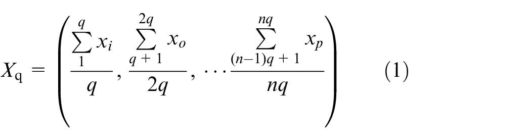
For a section of vibration signal y, x is the amplitude of the corresponding timestamp. This value depends on the timing relationship, so each amplitude has its own number. The piecewise aggregation approximation method is used here for encoding, and then converted into a polar expression, the GAF feature map is generated finally. Start by taking the average of every Q points to aggregate the time series. As shown in formula (1), we will get a new sequence $X_{q}$ , $X_{q} = [x_{q 1}, x_{q 2}, . . ., x_{qn}]$ .

X_{q} = (\frac{\sum_{1}^{q} x_{i}}{q}, \frac{\sum_{q + 1}^{2 q} x_{o}}{2 q}, \dots \frac{\sum_{(n - 1) q + 1}^{nq} x_{p}}{nq})

(1)

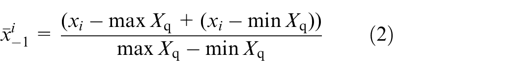
Then use the formula (2) to normalize the new sequence, and scale the time series value to the [−1,1] interval to make it standard.

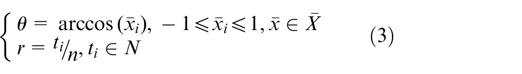
{\bar{x}}_{- 1}^{i} = \frac{(x_{i} - max X_{q} + (x_{i} - min X_{q}))}{max X_{q} - min X_{q}}

(2)

Use equation (3) to convert it into the expression of polar coordinates $\bar{X}$ .

{\begin{matrix} θ = \arccos ({\bar{x}}_{i}), - 1 \leq {\bar{x}}_{i} \leq 1, \bar{x} \in \bar{X} \\ r = t_{i} / n, t_{i} \in N \end{matrix}

(3)

$t_{i}$ is the timestamp and $n$ is a constant factor. Finally, formula (4) is used to generate two feature maps of the Gramian angular ummation (GASF) field and the Gramian angular difference field (GADF).

\begin{matrix} {\begin{matrix} G_{s} = \cos (θ_{i} + θ_{j}) \\ G_{s} = {\bar{X}}^{T} \cdot \bar{X} - {\sqrt{I - {\bar{X}}^{2}}}^{T} \sqrt{I - {\bar{X}}^{2}} \end{matrix} \\ {\begin{matrix} G_{D} = \sin (θ_{i} - θ_{j}) \\ G_{D} = {\sqrt{I - {\bar{X}}^{2}}}^{T} \cdot {\bar{X}}^{T} - \sqrt{I - {\bar{X}}^{2}} \end{matrix} \end{matrix}

(4)

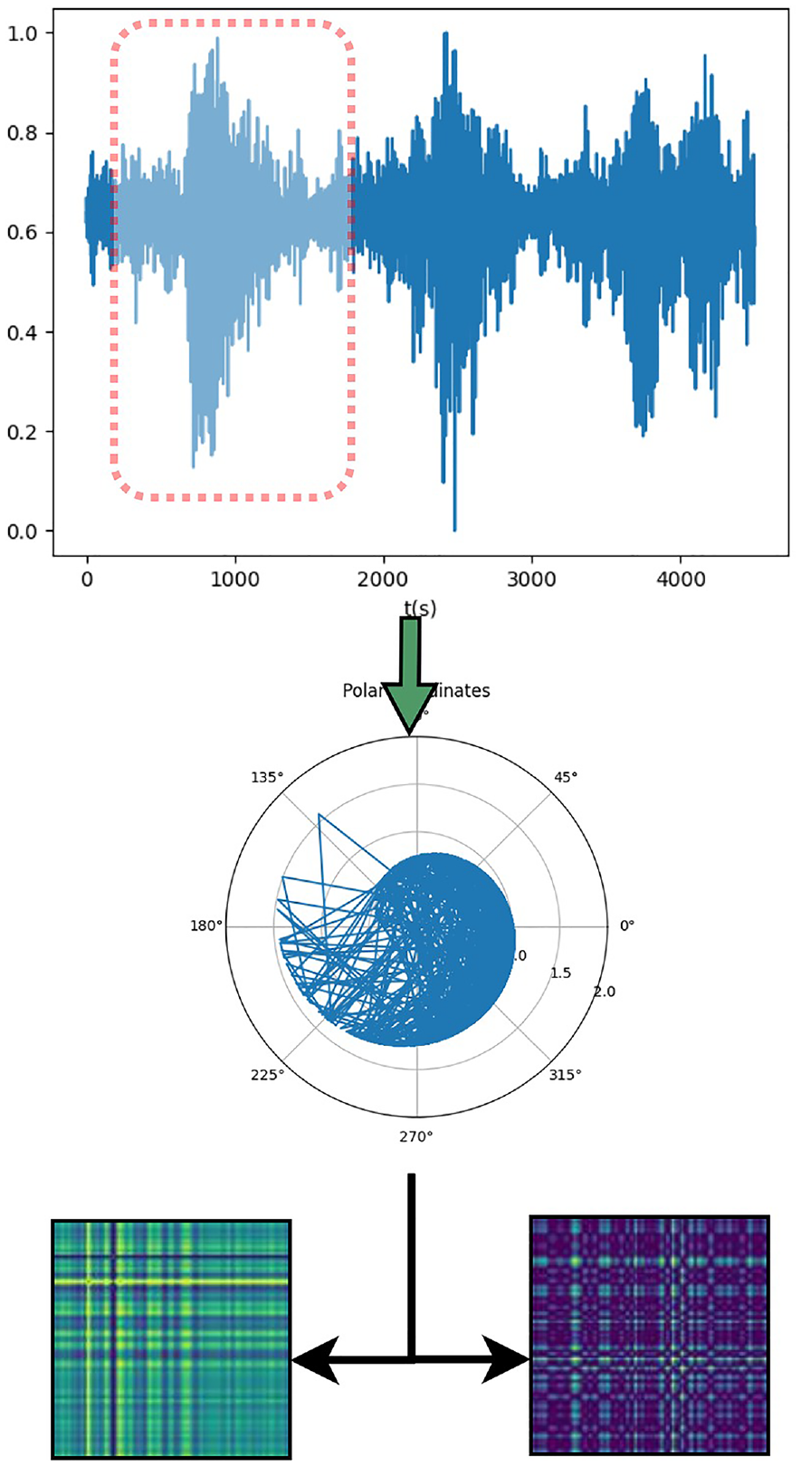
In the above formula: $I$ is the unit row vector; $\bar{X}$ is the row vector of $X$ ; ${\bar{X}}^{T}$ is the transpose vector of $X$ . The overall visualization process of GAF encoding is shown in Figure 1.

Figure 1.

GAF image coding.

Intensive mean teacher model

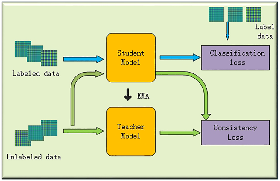
The average teacher model can efficiently utilize a large amount of unlabeled data and use the consistency regularization³⁴ method of unlabeled data to reduce the overfitting problem in semi-supervised deep learning. This model is suitable for classification tasks of two-dimensional data, and can also achieve better classification for large data sets. On this basis, this paper adopts the enhanced average teacher model to diagnose faults in gearbox.

In this method, the same two network structures will be trained at the same time, namely the teacher network and the student network. The training process is shown in Figure 2. First, the teacher network parameters are the exponential moving average (EMA) of the student network,³⁵ and the student network parameter update method is through gradient descent. In each round of training, the student network and teacher network train labeled data and unlabeled data respectively. The obtained predicted results are compared with the actual results and the total loss function is calculated. After the weight parameters of the student network are updated, they are averaged with the weight of the teacher network, and the teacher’s weight is continuously updated.

Figure 2.

Model training process.

The weight of the teacher network can be represented by $δ_{t}$ , and the weight of the student network can be represented by $δ_{s}$ . The exponential moving average formula is as follows:

δ_{t} = θ δ_{t} + (1 - η) δ_{t}

(5)

Where $θ \in (0, 1)$ is momentum. The loss of the student network consists of two parts, is shown in equation (6):

L_{s} = L_{a} + η L_{b},

(6)

Where $L_{a} = \sum_{i = 0}^{N} | f_{θ_{s}} (x_{i}^{l}) - y_{i}^{l} |$ represents the loss of supervision and $L_{b} = \sum_{i = 0}^{M} | f_{θ_{s}} (ϕ_{s} (x_{i}^{u})) - f_{θ_{t}} (ϕ_{t} (x_{i}^{u})) |$ represents the loss of unsupervised consistency. $| \cdot |$ refers to L1 distance. $ϕ_{s}$ represents the input augmentation to the student network, and $ϕ_{t}$ represents the input augmentation to the teacher network. Ideally, the simultaneously trained teacher network is usually better than the student network, and $L_{b}$ can provide effective supervision to train the student network on an unlabeled dataset. In this way, the output $y_{i}^{u} = f_{θ_{t}} (ϕ_{t} (x_{i}^{u}))$ of the teacher model can be called assume label. This kind of label may have errors, but after extensive testing, the final prediction effect of the teacher model has not been affected.

Fault diagnosis model based on GAF-MTDL

Improved student model and teacher model

Since the network structure of the teacher model and the student model are the same, it is crucial to choose a model with high classification accuracy and strong generalization ability. The more common deep neural network (DNN)³⁶ and the popular CNN are both excellent classification networks, and the processing effect of CNNs in the field of image and natural language processing is better.⁸ The GAF algorithm used in this paper happens to be an algorithm that converts 1D data into 2D images, so it can be understood as an image classification task. The image can actually be regarded as a matrix. During the training process, the model tries to analyze and understand the differences between different categories by itself, and then predict the label on the unknown image. In general, CNN has a three-layer structure: convolution, pooling and full connection (FC). The pooling convolution layer extracts the most obvious features, and the fully connected layer handles classification tasks. However, as the depth of the network increases, the convolutional neural network will suffer from problems such as gradient disappearance and network degradation.³⁷ The emergence of the residual neural network (ResNet) effectively alleviates these problems.It can speed up the training of the neural network, and greatly improve the generalization ability and robustness of the deep network.

The ResNet model³⁸ is an upgraded version of the CNN. Unlike all other publicly available CNNs, ResNet adds short connections outside the original convolutional layers to form residual blocks, which avoids the vanishing gradient problem that occurs as the network becomes more extensive and complex. There are various variants of ResNets, which have shown excellent performance in many tasks. In addition to the original ResNet-34,³⁹ ResNet-50,⁴⁰ and other network structures, there is also a residual based block convolutional neural network WideResNet. First of all, it has a wider network structure. Each residual block uses a relatively large convolution kernel and more output feature map channels, and the network becomes wider and deeper. It has better feature extraction ability and stronger expression ability than ordinary residual network. Secondly, its parameters of model are relatively small. Because it uses fewer Cartesian product connections, which can reduce the risk of overfitting. In addition, the large-scale network, low complexity and small amount of parameters of WideResNet can improve the generalization ability, adapt to different data sets and tasks, and have better cost performance. In conclusion, improving the model performance by increasing the width of WideResNet can not only keeps the computational complexity within an acceptable range, but also improves the feature extraction and expression capabilities, so as to achieve the balance between accuracy and computational complexity.

Considering the requirements of this article and the training time, there is a WideResNet network structure designed as shown in Figure 3. First, the convolution layer uses the 3 × 3 convolution kernel for convoluting, padding is 1, and the number of output channels is 16. Residual block 1 contains four basic blocks, the number of input and output channels are 16 and 32, and the stride is 1. The residual block 2 contains four basic blocks, the number of input and output channels is 32, 64, and the stride is 2. The residual block 3 contains four basic blocks, the number of input and output channels is 64, 128, and the stride is 2. Performing batch normalization on the output of the last layer of convolution, using ReLU as the activation function, performing global average pooling on the output, and then inputing it to the fully connected layer with an output dimension of 5. 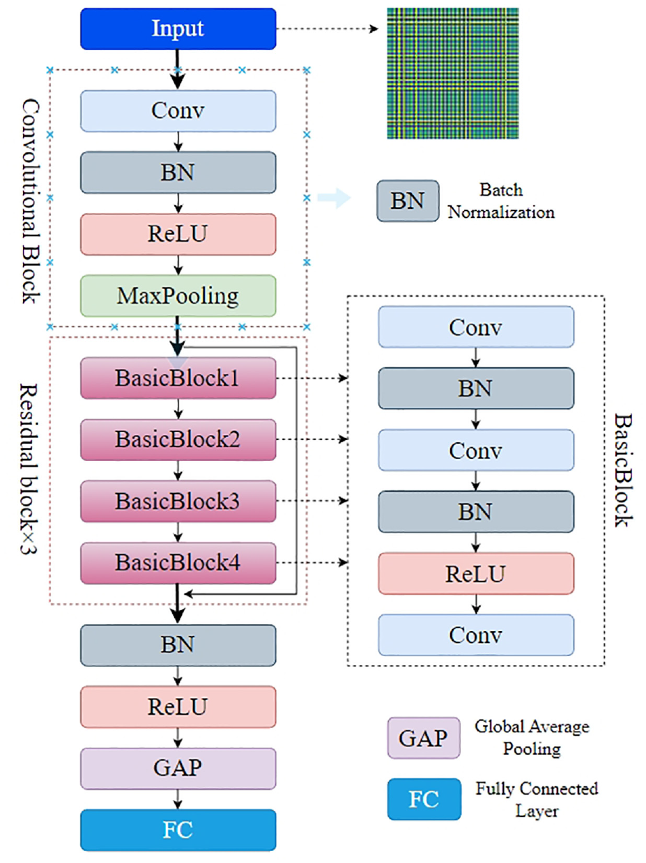Each of the basic block includes the following operations: first perform Batch Normalization on the input, then pass the ReLU activation function, and then use a $3 \times 3$ convolution kernel for convolution, padding is 1, and perform Batch Normalization on the output after convolution. Then pass the ReLu activation function, and then use a $3 \times 3$ convolution kernel for convolution, padding is 1. To prevent the model from overfitting, the dropout⁴¹ technique is introduced. Increasing the network width can effectively improve the accuracy of the network, but it also increases the model complexity and computing time. Therefore, this paper appropriately increases the depth and uses dropout technology while widening the network to achieve the better balance.

Figure 3.

WideResNet network structure.

GAF-MTDL fault diagnosis process

The overall process of fault diagnosis based on the GAF-MTDL model is shown in Figure 4, which can be described as:

Collect the fault signal and obtain the required GAF coding feature map. After the planetary gear test bench is arranged, gears with different fault types are implanted respectively, and vibration acceleration data under different fault conditions are collected using acquisition instruments and vibration acceleration sensors. The GAF algorithm is then used to convert the 1D time series vibration signal into a 2D feature map. Save all converted GAF encoded feature map data. Part of this batch of samples is labeled according to the proportion (20% of the label is defaulted for the first time), the data set is recorded as X1 (the corresponding label is Z1), and the other part of the unlabeled part is recorded as X2. After the data set is processed, it can be prepared for subsequent training of the network model.

First input this batch of data into the student network to get the output labels respectively: Ys1 and Ys2, and then construct the loss function for the labeled data X1, and the labeled classification loss function is L1(Z1, Zs1). Then input this batch of data into the teacher network model to get the output labels: Yt1 and Yt2, and construct the unsupervised loss function L2. In this paper, the total loss function L1 + L2 gradient descent is used to update the network parameters of the student network model and through exponential moving average to update the network parameters of the teacher network model.

Finally, the test set is used to evaluate the fault diagnosis effect of the GAF-MTDL network model, and the accuracy of different types of fault identification is visually displayed.

Figure 4.

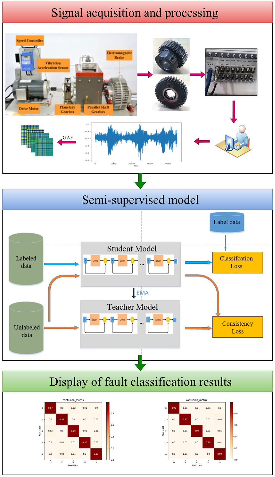
Fault diagnosis flowchart.

Experimental verification and result analysis

In order to verify the robustness and superiority of the proposed GAF-MTDL fault diagnosis model, four sets of experiments under different working conditions were carried out on the experimental bench built by our research group. In addition, in order to test its generalization ability, experiments were conducted on the open source data West Reserve University Bearing Dataset.

The development environment of this project uses NVIDIA RTX3060 GPU with 6 GB memory. The experimental environment is based on the Python language and pytorch1.13.1 version to build the neural network model.

Test data

This test is carried out on the DDS type power transmission fault diagnosis comprehensive test bench, and the physical picture is shown in Figure 5. It is directly connected to the sun gear through a coupling. The test device can simulate the faults of gears such as sun gears, planetary gears, and parallel shaft gears. This experiment simulates four types of faults of planetary gears, which are root cracks, tooth surface wear, broken teeth, and missing teeth. Adding the normal planetary gears is the five-sort problem.

Figure 5.

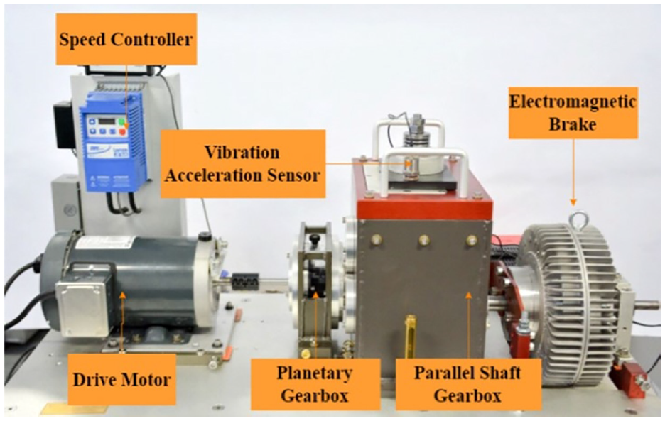
Fault diagnosis test bench.

The reduction ratio of the planetary gear is 4.571, which is the first stage reduction device. The parallel-axis gearbox (fixed-axis gear train) is the second/third-stage reduction device. The relevant parameters of the planetary gearbox mainly include: Zs = 28, Zp = 36, Zr = 100, Z1 = 29, Z2 = 100, Z3 = 36, Z4 = 90. A schematic diagram of its transmission system is shown in Figure 6.

Figure 6.

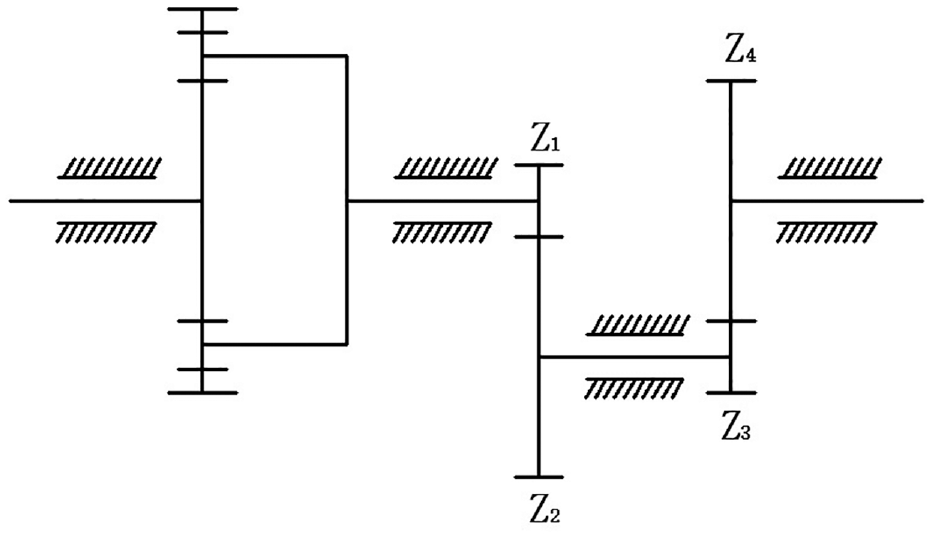
Transmission system diagram.

The sampling frequency is 10,000 Hz, and four operating conditions are set, the input shaft speed is 1800 and 2400 r/min, the system load is 0 and 30 N·m, and the other experimental conditions are the same. The sampling time of each operating condition is about 15 s, and the number of sampling points is 1,536,000. The parameters of the GAF encoding algorithm are set as follows: the length of the sampling window is 500, the step size of the sliding window is 500, the GAF method is selected as GADF,⁴² and there is no overlapping sampling. The ratio of training set and test set is set to 7:3. As shown in Figure 7, it is the GAF characteristic map generated by the fault signal sample under the load condition of 2400 r/min speed and 30 N·m. In fact, when observing the transformed characteristic map, the naked eye can see that the fault characteristics of missing teeth are the most obvious, followed by broken teeth and cracks, while healthy gears and worn gears are relatively weak. It also indirectly reflects that damaged gears will increase many fault characteristics.

Figure 7.

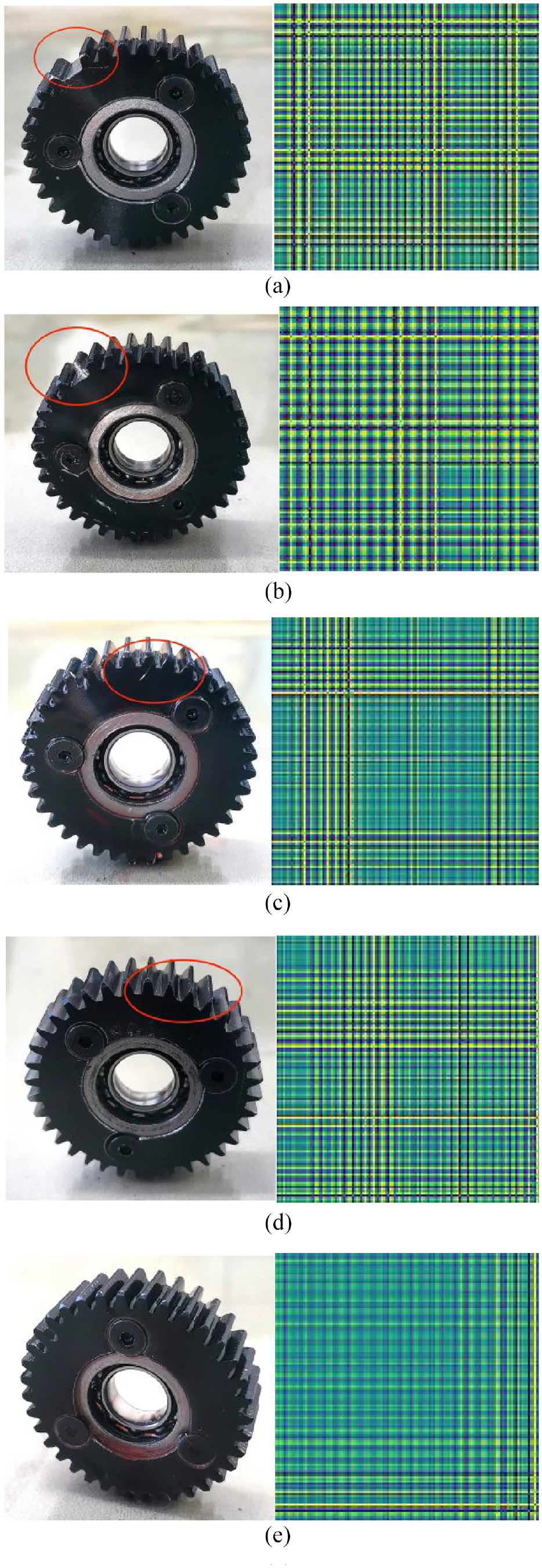
Gear physical map and GAF feature map: (a) missing tooth failure-0, (b) broken tooth failure-1, (c) tooth root crack-2, (d) tooth surface wear-3, and (e) health gear-4.

Model validation under different working conditions

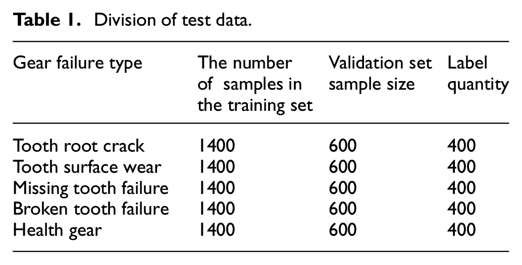
The data information of the test bench is shown in Table 1 below.

Table 1.

Division of test data.

Gear failure type	The number of samples in the training set	Validation set sample size	Label quantity
Tooth root crack	1400	600	400
Tooth surface wear	1400	600	400
Missing tooth failure	1400	600	400
Broken tooth failure	1400	600	400
Health gear	1400	600	400

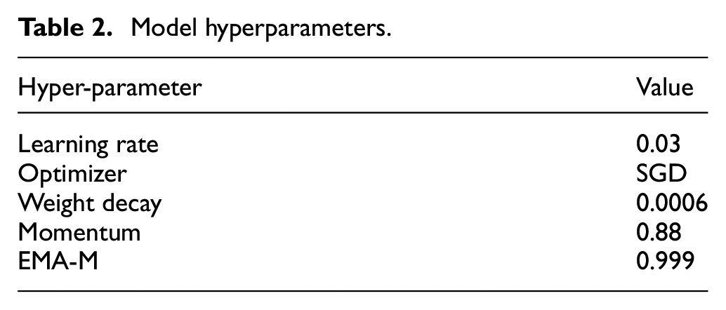
The semi-supervised model adopts MTDL, the training cycle is set to 30,000 steps, and the optimizer is selected as SGD. The specific hyperparameters are shown in Table 2. Import the prepared training set into the GAF-MTML model for training. During the training process, the data is saved every 500 steps, and the optimal model is saved when the training reaches 30,000 steps. After the iterative training is completed, the validation set is used to test the diagnostic effects of four different working conditions. The fault diagnosis accuracy rates are 97.63%, 98.22%, 97.28%, and 96.46% respectively.

Table 2.

Model hyperparameters.

Hyper-parameter	Value
Learning rate	0.03
Optimizer	SGD
Weight decay	0.0006
Momentum	0.88
EMA-M	0.999

As shown in Figure 8(a)–(d), they are the confusion matrix of fault classification under four working conditions. The first working condition is speed 1800 r/min and load 0 N.m (1800-0), The second working condition is speed 2400 r/min and load 0 N.m (2400-0), The third working condition is speed 1800 r/min and load 30 N.m (1800-30), The fourth working condition is that the speed is 2400 r/min and the load is 30 N.m (2400-30). 0 is missing tooth fault, 1 is broken tooth fault, 2 is tooth root crack, 3 is tooth surface wear, and 4 is healthy gear. The prediction accuracy and diagnosis errors of the model for each type of fault can be obtained from the confusion matrix. At the same time, according to the confusion matrix, when the label rate is only 20%, the fault diagnosis accuracy of any type of gear under any working condition can reach more than 96%.

Figure 8.

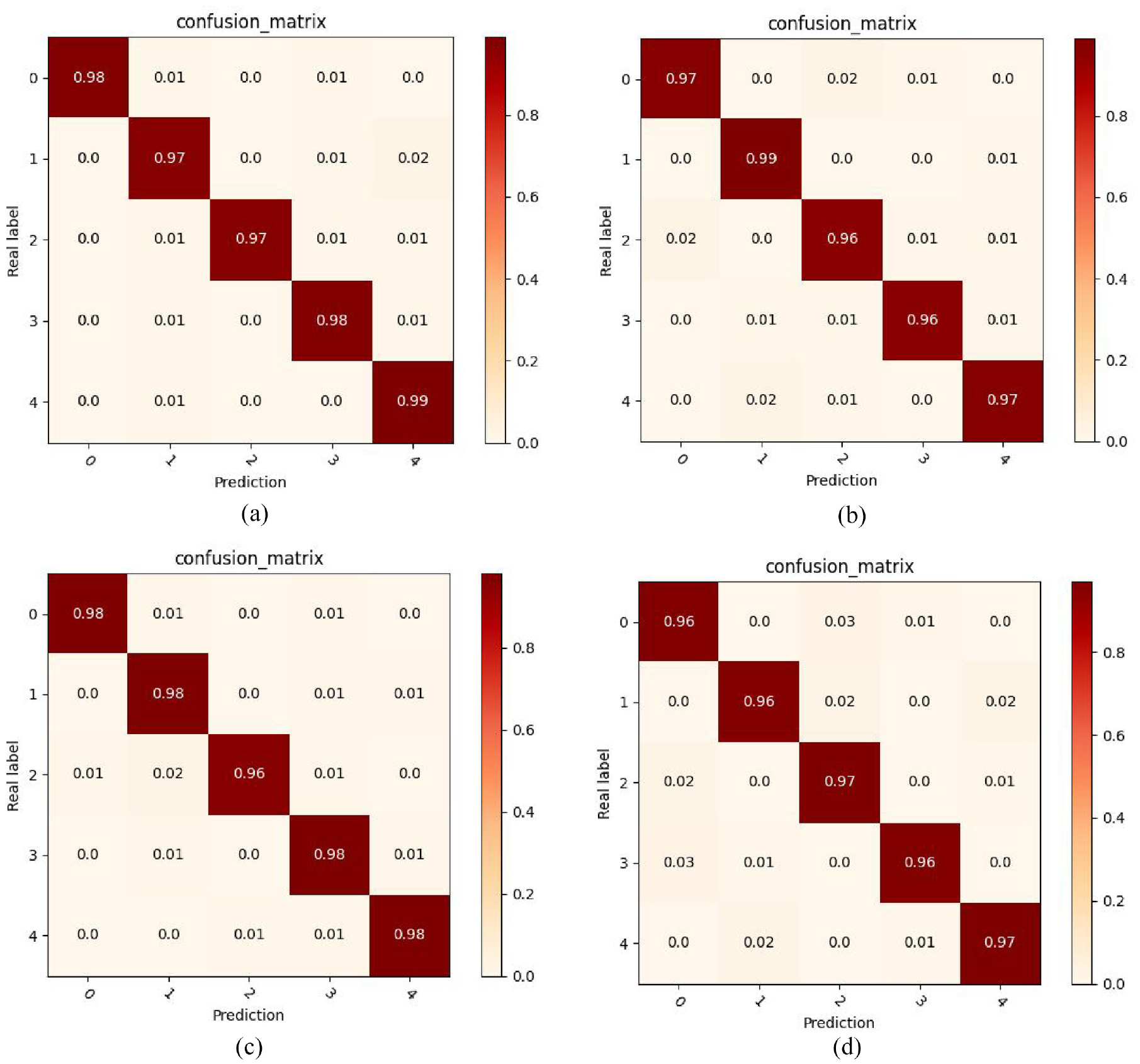
Gear classification confusion matrix for four working conditions: (a) 1800-0 working condition classification confusion matrix, (b) 2400-0 working condition classification confusion matrix, (c) 1800-30 working condition classification confusion matrix, and (d) 2400-30 working condition classification confusion matrix.

Comparative test analysis of different label rates

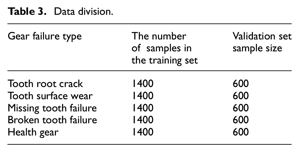
In addition, the test was carried out under the working condition of 2400 r/min and 30 N·m load, and the label rate of 2%, 5%, 10%, 15%, and 20% respectively. The detailed division of the data set is shown in Table 3. After multiple groups of training, the precision comparison chart and loss comparison chart is shown in Figure 9(a) and (b).

Table 3.

Data division.

Gear failure type	The number of samples in the training set	Validation set sample size
Tooth root crack	1400	600
Tooth surface wear	1400	600
Missing tooth failure	1400	600
Broken tooth failure	1400	600
Health gear	1400	600

Figure 9.

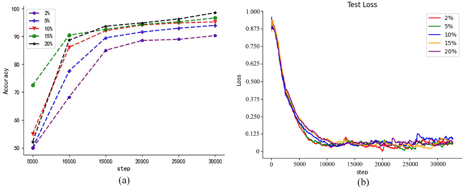
Classification accuracy curve and loss curve under different labeling rates: (a) comparison curve of gear accuracy change under different labeling rates and (b) comparison curve of gear loss change under different tag rates.

As can be seen from Figure 9, as the marking rate increases, the fault diagnosis effect gradually becomes better, which proves that the amount of marked data greatly affects the fault diagnosis effect. In addition, it can be clearly seen that under five different label rates, the GAF-MTDL fault diagnosis model’s identification accuracy of faulty gears is above 85%. Among them, the GAF-MTDL model has achieved a diagnostic accuracy of more than 90% at labeling rates of 5%, 10%, 15%, and 20%. What’s more, it has achieved better diagnostic results when the labeling rate is only 2%, indicating that this method can accurately identify faults with very few labels.

Comparison test of different image coding methods

In order to evaluate the advantages of using the GAF image encoding method in the MTDL network, we selected several existing 1D time series data upscaling methods. Such as time-frequency diagram (TFD),⁴³ relative position matrix (RPM),⁴⁴ Markov transition field (MTF),⁴⁵ etc. Figure 10 shows the accuracy under different image encoding method inputs. In general, when the label rate is only 10%, GADF-MTDL, GASF-MTDL, MTF-MTDL, RPM-MTDL, TFD-MTDL, these five methods can all achieve more than 80% fault identification accuracy. With a label rate of 15%, the fault identification accuracy rate has reached about 90%. It proves that the MTDL model has good adaptability in the recognition of different types of feature maps, and also shows that the model proposed in this paper has a strong ability to recognize two-dimensional data. It is also worth mentioning that whether the label rate is 10%, 15%, or 20%, the overall accuracy of the GADF-MTDL method significantly exceeds other methods. This shows that the GADF-MTDL method exhibits excellent performance on this task. It has more accurate classification and prediction capabilities than other methods, resulting in higher overall accuracy.

Figure 10.

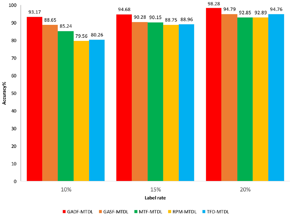
Accuracy under different image encodings.

Comparison of different deep learning algorithms

To verify the superiority of the semi-supervised algorithm in fault diagnosis, we compared it with several supervised methods, using the same amount of labeled data. Through such a comparison, we can evaluate whether the semi-supervised algorithm has better performance under the same data conditions. Several commonly used supervised classification algorithms, such as Vgg,⁴⁶ Alexnet,⁴⁷ SAE,⁴⁸ etc. The verification set data was used for verification, and the average accuracy was obtained from five experiments respectively. The specific comparison results have been recorded in Table 4. We can get detailed comparative data by looking at this table.

Table 4.

Compared with supervised diagnosis results.

Model	Accuracy (%)
	200 Label	400 Label
GADF-Vgg16	80.55	94.61
GADF-Alexnet	79.07	93.65
GADF-SAE	80.85	92.36
GADF-MTDL	92.67	98.22

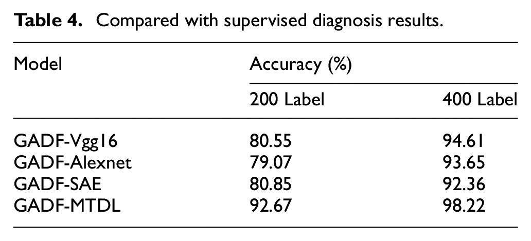
It is obvious from the above table that when 200 labeled numbers are used, the diagnostic accuracy of the three supervised algorithms is about 80%, and the diagnostic effect is relatively general. So far, the GADF-MTDL method has accomplished a diagnostic accuracy of 92.67%, showing very good results. When the number of labels reaches 400, the other three methods also achieve an accuracy of more than 90%. Although there are some gaps compared with the GADF-MTDL method, it can still be considered that they perform well in diagnostic effects. The side shows that the supervised algorithm is very sensitive to the diagnosis effect in the number of labels, and this further validates that our semi-supervised diagnostic method has a stronger effect. When the number of labels is scarce, the performance of semi-supervised GAF-MTDL can still remain relatively stable. First of all, the advantage of semi-supervised algorithms is that they fully utilize the potential of unlabeled data and play an auxiliary role without labels. Secondly, when the available training sample data is limited in size, the use of supervised models is prone to overfitting problems. Therefore, the semi-supervised diagnostic approach introduced in this paper demonstrates greater versatility and dependability within the industrial sector.

Finally, considering the superiority of the semi-supervised algorithm of this model, a comparative test is conducted with three semi-supervised algorithms. Self-training,⁴⁹ Co-training,⁵⁰ and SGAN⁵¹ are relatively mature semi-supervised models. In this study, the labeling rate was set to 20%, and the same dataset was used during training, while an independent test set was used for evaluation during the testing phase. In order to reduce the impact of accidental errors, each algorithm was trained independently 10 times under different initialization conditions, and the average of its accuracy was taken as the final result. The ultimate accuracy comparison findings are depicted in Figure 11. The accuracy of GADF + Self-training, GADF + Co-training, and GADF + SGAN is basically about 95%. The diagnostic accuracy of these three semi-supervised algorithms has achieved considerable results. In fact, they have given full play to the advantages of semi-supervised, but the accuracy rate of GADF + MTDL is as high as 98.22%, and the effect is stronger, which can better illustrate the strength of GADF-MTDL algorithm. In general, by comparing several supervised algorithms and several commonly used semi-supervised algorithms, the semi-supervised algorithm is bound to be better than the supervised algorithm when the number of labels is limited. This is because semi-supervised algorithm can fully amplify the ability to assist model training on unlabeled data.

Figure 11.

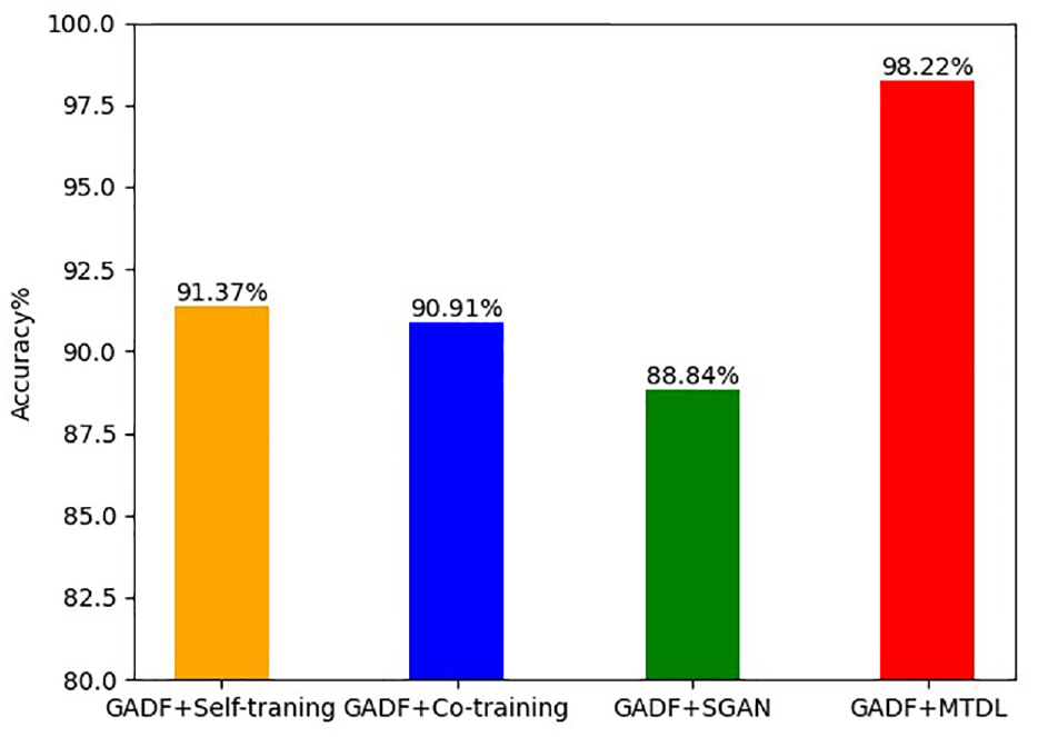
Semi-supervised algorithm comparison diagnosis results.

Generalization capability verification

Introduction to Western Reserve University Dataset

The data set we used is the Case Western Reserve University bearing data set, in which some representative samples were selected for analysis. There are four working conditions in total, one load corresponds to one speed, zero horsepower – 1797 r/min, one horsepower – 1772 r/min, two horsepower – 1750 r/min, three horsepower – 1730 r/min. What is being tested this time is the driving end of the bearing, and the sampling frequency is 12 kHz. There are three types of bearing faults: rolling element faults, inner ring faults and outer ring faults. Each fault diameter comes in three different sizes, namely 0.1788, 0.3556, and 0.5334 mm, covering a total of 10 different situations. In order to facilitate testing, faults are defined as first-level, second-level, and third-level faults according to their size. The healthy one are recorded as NOR, and the others are recorded as: rolling element first-level fault BA1, rolling element second-level fault BA2, rolling element third-level fault BA3, inner ring first-level fault IN1, inner ring second-level fault IN2, inner ring third-level fault IN3, outer ring first-level fault OUT1, outer ring second-level fault OUT2, outer ring third-level fault OUT3 (Figure 12).

Figure 12.

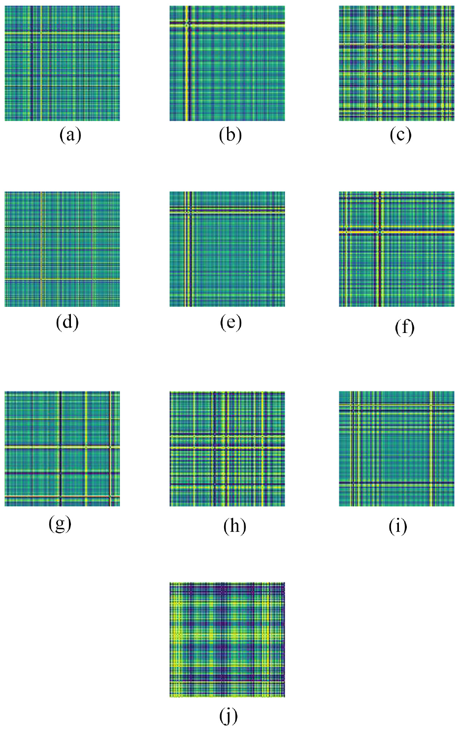
GAF characteristic map of the bearing of Western Reserve University: (a) BA1, (b) BA2, (c) BA3, (d) IN1, (e) IN1, (f) IN1, (g) OUT1, (h) OUT1, (i) OUT1, and (j) NOR.

The sampling window length is set to 500, the sliding window step is 60, the GAF image encoding method is GADF, and 2000 samples are generated for each fault type.

Model training and verification analysis

According to the conversion process of the above-mentioned GAF algorithm, the samples were made into a GAF sample set. Select seven-tenths of the data for training and the rest for testing as shown in Table 5.

Table 5.

Dataset structure.

Fault type	Training samples	Verification sample
7 Mils ball faults	1400	600
14 Mils ball faults	1400	600
21 Mils ball faults	1400	600
7 Mils inner race faults	1400	600
14 Mils inner race faults	1400	600
21 Mils inner race faults	1400	600
7 Mils outer race faults	1400	600
7 Mils outer race faults	1400	600
7 Mils outer race faults	1400	600
Normal	1400	600

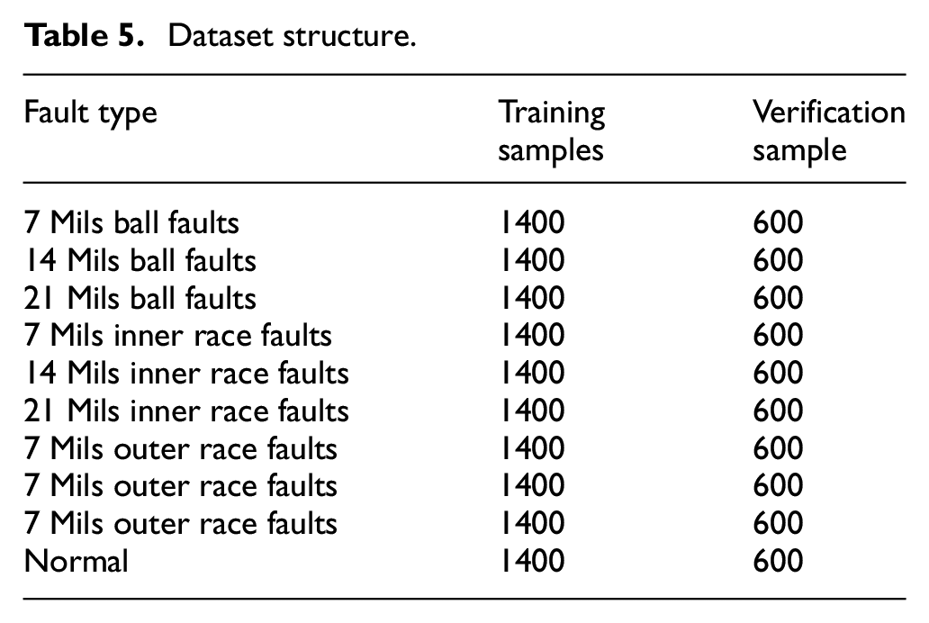
GAF-MTDL model parameters are the same as the above test selection, only the number of categories is changed from 5 to 10. The number of training steps is consistent with the above gear test, and the data is saved every 5000 steps. The optimizer is chosen as SGD, and the hyperparameters used are also consistent. This test also verifies its tests under the conditions of five different labeling rates. Figure 13(a) and (b) show the accuracy rate and loss function curves under five different label rates respectively. The accuracy of sample fault diagnosis under five different labeling rates is 99.98%, 99.71%, 99.00%, 97.21%, 90.23%, respectively. Obviously, the model suggested in this research paper shows strong adaptability and robustness, and efficient diagnosis effect on open source data sets.

Figure 13.

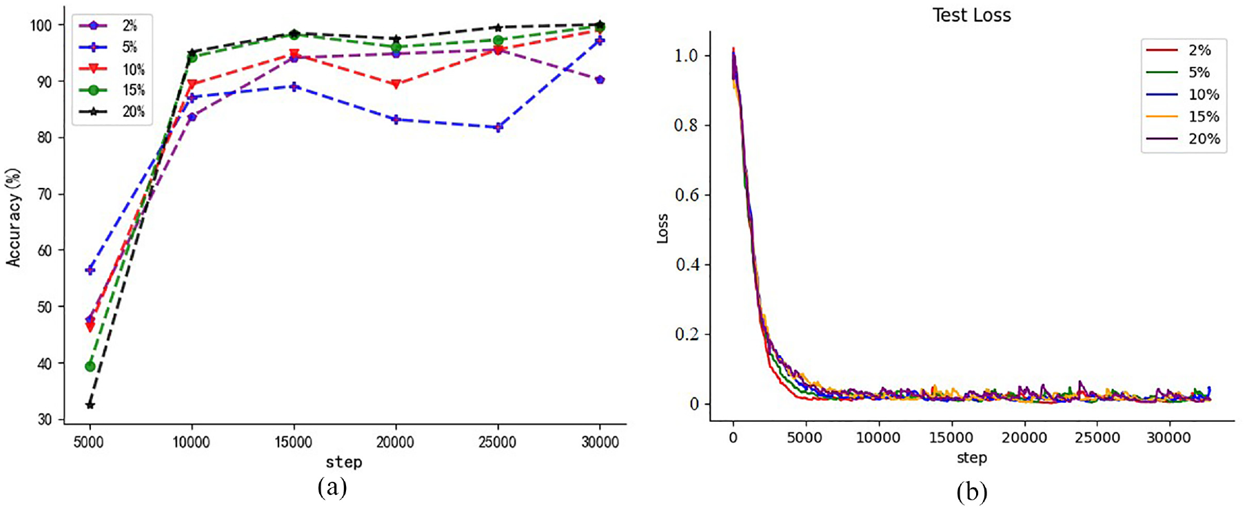
Accuracy rate change and loss change curve: (a) comparison curve of bearing accuracy change and (b) comparison curve of bearing loss change.

In order to accurately evaluate the recognition performance of various fault types under 20% labeling rate, we provide a diagram of the bearing classification confusion matrix, which is specifically shown in Figure 14. This confusion matrix can help us to understand the classification results of different fault types more clearly. The fault recognition accuracy of BA1 and BA2 has reached more than 99% recognition accuracy. OUT3 has also reached more than 98% fault recognition accuracy. The rest of the fault types are basically close to 100% diagnosis accuracy. It is further verified that the model has outstanding performance in fault identification, indicating that it has strong anti-interference and generalization capabilities. These findings strengthen the reliability and validity of the model in practical engineering applications.

Figure 14.

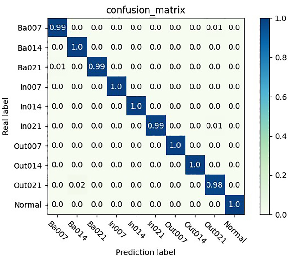
Twenty percent label rate bearing classification confusion matrix.

Conclusion

In order to overcome the problems of high labeling cost, scarcity of labeled samples, and low accuracy in fault diagnosis in practical applications, this study proposes an improved fault diagnosis method based on semi-supervised deep learning and GAF model. Through experimental verification and comparative studies with other methods, the following results were obtained:

(1) This paper proposes a new fault diagnosis method, which uses the GAF algorithm to increase the dimension of 1D time series vibration signals as input. This method makes full use of the advantages of wide residual neural network in image recognition, thus the effect of fault identification is significantly improved.

(2) This method combines the efficiency of supervised algorithms and extensiveness of unsupervised networks. The network model can be used in many places and has strong generalization ability.

(3) Compared with other semi-supervised learning methods, the MTDL network has a higher diagnostic accuracy rate. In the extreme case of only 5% label data for each class, it still has a diagnostic accuracy rate of 90.21%.

(4) The GAF-MTDL network can use less labeled data to achieve the same or even higher diagnostic accuracy than the supervised learning method.

(5) The GAF-MTDL network model has strong robustness and generalization ability, and has excellent diagnostic results no matter what working conditions or test benches are used.

Future work will further study the performance of other different types of monitoring signals in intelligent fault diagnosis, as well as fault diagnosis methods based on multi-source data decision fusion. In order to quickly and accurately identify the faults of various components of the mechanical equipment system.

Footnotes

Declaration of conflicting interests

The author(s) declared no potential conflicts of interest with respect to the research, authorship, and/or publication of this article.

Funding

The author(s) disclosed receipt of the following financial support for the research, authorship, and/or publication of this article: This research work was supported by Applied Basic Research Project of Shanxi Province under Grant No. 20210302124204, Key Research and Development Project of Shanxi Province under Grant No. 202102010101009 and Grant No. 202102010101006, and in part by the National Natural Science Foundation of China under Grant No. 52175108.

ORCID iDs

Peng Zhao

Feng Li

References

Wang

. K-nearest neighbors based methods for identification of different gear crack levels under different motor speeds and loads: Revisited. Mech Syst Signal Process 2016; 70–71: 201–208.

Yang

Liu

, et al. Gear fault diagnosis based on support vector machine optimized by artificial bee colony algorithm. Mech Mach Theory 2015; 90: 219–229.

Wang

Shao

. Crack fault classification for planetary gearbox based on feature selection technique and K-means clustering method. Chin J Mech Eng 2018; 31(1): 1–11.

Wang

Yang

, et al. Subdomain adaptation transfer learning network for fault diagnosis of roller bearings. IEEE Trans Ind Electron 2022; 69(8): 8430–8439.

Pang

Xue

Jiang

, et al. An investigation into fault diagnosis of planetary gearboxes using a bispectrum convolutional neural network. IEEE ASME Trans Mechatron 2021; 26(4): 2027–2037.

Xiao

Shao

Feng

, et al. Towards trustworthy rotating machinery fault diagnosis via attention uncertainty in Transformer. J Manuf Syst 2023; 70: 186–201.

Yao

Han

. Data-driven lithium-ion batteries capacity estimation based on deep transfer learning using partial segment of charging/discharging data. Energy 2023; 271: 127033.

Wang

Kuen

, et al. Recent advances in convolutional neural networks. Pattern Recognit 2018; 77: 354–377.

Wang

Zhou

, et al. Bearing fault diagnosis method based on adaptive maximum cyclostationarity blind deconvolution. Mech Syst Signal Process 2022; 162: 108018.

10.

Feng

Chen

, et al. A cyclostationarity-based wear monitoring framework of spur gears in intelligent manufacturing systems. Struct Health Monit 2023; 22: 3108.

11.

Zhang

Tang

Deng

, et al. A hybrid attention improved ResNet based fault diagnosis method of wind turbines gearbox. Measurement 2021; 179: 109491.

12.

Zhang

Pang

Zhao

, et al. A new method based on encoding data probability density and convolutional neural network for rotating machinery fault diagnosis. IEEE Access 2023; 11: 26099–26113.

13.

Feng

Wang

, et al. A novel order spectrum-based Vold-Kalman filter bandwidth selection scheme for fault diagnosis of gearbox in offshore wind turbines. Ocean Eng 2022; 266: 112920.

14.

Feng

Zhang

, et al. Digital twin-driven intelligent assessment of gear surface degradation. Mech Syst Signal Process 2023; 186: 109896.

15.

Nettleton

Orriols-Puig

Fornells

. A study of the effect of different types of noise on the precision of supervised learning techniques. Artif Intell Rev 2010; 33: 275–306.

16.

Glielmo

Husic

Rodriguez

, et al. Unsupervised learning methods for molecular simulation data. Chem Rev 2021; 121(16): 9722–9758.

17.

Chen

Shao

Xiao

, et al. Collaborative fault diagnosis of rotating machinery via dual adversarial guided unsupervised multi-domain adaptation network. Mech Syst Signal Process 2023; 198: 110427.

18.

Han

Xie

Pei

. Semi-supervised adversarial discriminative learning approach for intelligent fault diagnosis of wind turbine. Inf Sci 2023; 648: 119496.

19.

Zaman

SMK

Liang

. An effective induction motor fault diagnosis approach using graph-based semi-supervised learning. IEEE Access 2021; 9: 7471–7482.

20.

Yuan

Liu

. Semi-supervised learning and condition fusion for fault diagnosis. Mech Syst Signal Process 2013; 38(2): 615–627.

21.

Zhao

Ball

Mosesian

, et al. Graph-based semi-supervised learning for fault detection and classification in solar photovoltaic arrays. IEEE Trans Power Electron 2015; 30(5): 2848–2858.

22.

Zhang

Cheng

, et al. A hybrid classification autoencoder for semi-supervised fault diagnosis in rotating machinery. Mech Syst Signal Process 2021; 149: 107327.

23.

Zhang

Liu

, et al. Feature extraction for rolling element bearing fault diagnosis utilizing generalized S transform and two-dimensional non-negative matrix factorization. J Sound Vib 2011; 330(10): 2388–2399.

24.

Zhang

Sun

Guo

, et al. A new bearing fault diagnosis method based on modified convolutional neural networks. Chin J Aeronaut 2020; 33(2): 439–447.

25.

Wang

Shang

. Kalman filter based fault detection for two-dimensional systems. J Process Control 2015; 28: 83–94.

26.

Han

Zhang

Sun

, et al. A new bearing fault diagnosis method based on capsule network and Markov transition field/Gramian angular field. Sensors 2021; 21(22): 7762.

27.

Cui

Zhong

Zheng

, et al. A lightweight model for bearing fault diagnosis based on gramian angular field and coordinate attention. Machines 2022; 10(4): 282.

28.

Lyu

Huo

Cheng

, et al. Distributed optical fiber sensing intrusion pattern recognition based on GAF and CNN. J Light Technol 2020; 38(15): 4174–4182.

29.

Huynh

Nguyen

. Joint age estimation and gender classification of Asian faces using wide ResNet. Comput Sci 2020; 1(5): 284.

30.

Peng

Tse

Chu

. An improved Hilbert–Huang transform and its application in vibration signal analysis. J Sound Vib 2005; 286(1–2): 187–205.

31.

Kong

, et al. A residual convolutional neural network with multi-block for appliance recognition in non-intrusive load identification. Energy Build 2023; 281: 112749.

32.

Wang

Oates

. Encoding time series as images for visual inspection and classification using tiled convolutional neural networks. In: Proceedings of the AAAI conference on artificial intelligence, TX, USA, 25–30 January 2015, vol. 1.

33.

Nagem

Qahwaji

Ipson

, et al. Predicting solar flares by converting goes x-ray data to gramian angular fields (GAF) images. In: Proceedings of the world congress on engineering, London, UK, 4–6 July 2018, Vol. 1.

34.

Yeung

. Addressing two problems in deep knowledge tracing via prediction-consistent regularization. In: Proceedings of the fifth annual ACM conference on learning at scale, London, UK, 26–28 June 2018, pp.5–10.

35.

Haynes

Corns

Venayagamoorthy

. An exponential moving average algorithm. In: Proceedings of the 2012 IEEE congress on evolutionary computation, Brisbane, Australia, 10–15 June 2012, pp.1–8.

36.

Borkar

Karam

. DeepCorrect: correcting DNN models against image distortions. IEEE Trans Image Process 2019; 28(12): 6022–6034.

37.

Shah

Kadam

Shah

, et al. Deep residual networks with exponential linear unit. In: Proceedings of the third international symposium on computer vision and the internet, Jaipur, India, 21–24 September 2016, pp.59–65.

38.

Liu

Tao

. Why resnet works? Residuals generalize. IEEE Trans Neural Netw Learn Syst 2020; 31(12): 5349–5362.

39.

Gao

, et al. A transfer residual neural network based on ResNet-34 for detection of wood knot defects. Forests 2021; 12(2): 212.

40.

Wen

Gao

. A transfer convolutional neural network for fault diagnosis based on ResNet-50. Neural Comput Appl 2020; 32: 6111–6124.

41.

Srivastava

Hinton

Krizhevsky

, et al. Dropout: a simple way to prevent neural networks from overfitting. J Mach Learn Res 2014; 15(1): 1929–1958.

42.

Xiao

Chen

Zhu

. GADF/GASF-HOG:feature extraction methods for hand movement classification from surface electromyography. J Neural Eng 2020; 17(4): 046016.

43.

Sun

Yang

Chen

, et al. Gear fault diagnosis based on the structured sparsity time-frequency analysis. Mech Syst Signal Process 2018; 102: 346–363.

44.

Chen

Shi

. A deep learning framework for time series classification using relative position matrix and convolutional neural network. Neurocomputing 2019; 359: 384–394.

45.

Bugueño

Molina

Mena

, et al. Harnessing the power of CNNs for unevenly-sampled light-curves using Markov transition field. Astron Comput 2021; 35: 100461.

46.

Tammina

. Transfer learning using VGG-16 with deep convolutional neural network for classifying images. Int J Sci Res Publ 2019; 9(10): 143–150.

47.

Ismail Fawaz

Lucas

Forestier

, et al. Inceptiontime: finding alexnet for time series classification. Data Min Knowl Discov 2020; 34(6): 1936–1962.

48.

, et al. Feature learning based on SAE–PCA network for human gesture recognition in RGBD images. Neurocomputing 2015; 151: 565–573.

49.

Zhou

. Self-training from labeled features for sentiment analysis. Inf Process Manag 2011; 47(4): 606–616.

50.

Yaslan

Cataltepe

. Co-training with relevant random subspaces. Neurocomputing 2010; 73(10-12): 1652–1661.

51.

Zhang

Shi

Zhu

, et al. Active semi-supervised learning based on self-expressive correlation with generative adversarial networks. Neurocomputing 2019; 345: 103–113.

Gearbox fault diagnosis method based on improved semi-supervised MTDL and GAF

Abstract

Keywords

Introduction

Related algorithm theory

GAF image coding

Intensive mean teacher model

Fault diagnosis model based on GAF-MTDL

Improved student model and teacher model

GAF-MTDL fault diagnosis process

Experimental verification and result analysis

Test data

Model validation under different working conditions

Comparative test analysis of different label rates

Comparison test of different image coding methods

Comparison test of different image coding methods

Comparison of different deep learning algorithms

Generalization capability verification

Introduction to Western Reserve University Dataset

Model training and verification analysis

Conclusion

Footnotes

Declaration of conflicting interests

Funding

ORCID iDs

References