
Abstract
Small and imbalanced fault samples have a profound impact on the diagnostic performance of a model in the process of locating and quantifying the rolling bearing damage of aeroengines in practice. Therefore, a Siamese Convolutional Neural Network-Bidirectional Long Short-Term Memory (CNN-BiLSTM) model was proposed in this paper. Random selection and cross combination methods were used to augment and balance sample sizes at first. Then, two weight-sharing CNN-BiLSTM models were used for adaptive extraction and distance measurement of weak fault features. Finally, the fault classification was performed based on feature distance. Model performance was verified using simulated fault test data of rolling bearings. The results showed that the Siamese CNN-BiLSTM model could achieve an accuracy of up to 96.0% for quantitative diagnosis and 98.0% for location diagnosis. This model was also capable of solving the imbalanced classification of samples and made it possible to transfer between different rotating speeds and working conditions.
Introduction
Rolling bearings have a significant influence on the safety in use, service life, and reliability of rotary machines including aeroengines. Surface damage is one major failure form of rolling bearings, and the damage site and area directly reflect the operating state of rolling bearings, further affecting the reliability of aeroengines. Among the many commonly used methods for monitoring the condition of aircraft engine rolling bearings, vibration analysis 1 has been widely used due to its advantages of simple measurement, high accuracy, and low cost. Thus, accurate evaluation of the size and location of rolling bearing damage based on vibration monitoring data has important implications for early diagnosis of bearing faults and prediction of the remaining useful life of bearings.
Conventional vibration signal analysis methods 2 and machine learning methods 3 require a large quantity of priori knowledge, and are influenced greatly by noise in practice. Thus, these methods have weak robustness and poor generalization ability. Due to great superiority in adaptive extraction of features, deep learning has become a research hotpot in recent years, attracting wide attention and leading to extensive discussion.4,5
However, rolling bearing data collected from aeroengines during actual operation are mostly normal, and the scarcity and imbalanced distribution of fault samples greatly lower the performance of deep learning models. How to locate and quantify faults with small and imbalanced samples and improve the generalization performance of models in complex working conditions and a changing rotating speed is of great engineering significance to the detection and prediction of rolling bearing faults.6,7
A series of studies have been proposed to address the problem of imbalanced diagnosis and few samples: Hu et al. 8 used order tracking and resampling methods to process bearing data at different speeds, and the average accuracy was much better than traditional SVM methods under six cross working conditions with few samples. Li et al. 9 proposed an autoencoder embedded dictionary learning approach for nonlinear industrial process fault diagnosis, which outperforms several dictionary learning approaches and some other nonlinear fault diagnosis methods. Berenji et al. 10 trained an autoencoder with unlabeled samples, and applied a contrastive learning-based post-training to make use of limited available labeled samples to improve the rolling bearing feature set discriminability.
However, most existing deep learning methods for fault diagnosis only focus on prediction accuracy without considering the limitation of both small and imbalanced samples of rolling bearing. Besides, specialized small sample learning networks lack reasonable embedding modules and have certain shortcomings such as insufficient feature extraction ability.
The recently emerging meta-learning method11,12 guides the learning of new tasks by previous knowledge and experience. This method is aimed at teaching the model how to learn, namely, to catch the essential features of data though comparing different small sample data and thus to acquire the most information with the least memory. Many studies13,14 on meta-learning show that meta-learning models have strong generalization ability, high accuracy and good robustness for small-sample and even single-sample learning problems.
In meta-learning, metric learning-based SiameseNets (SNs) 15 extract features with two weight-sharing networks of the same structure and define the classification criteria based on distance metrics. As a useful meta-learning network with high performance, SNs are extensively applied in the fields of target tracking16,17 and machine translation, 18 etc., but there are few studies on their application in the estimation of surface damage of aircraft engine rolling bearings.
In the location and quantitative detection of rolling bearing damage, SNs have several advantages. Firstly, SNs not only extract the features from input samples, but also find similarities between two samples by calculating their distance. With a unique structure, SNs are able to highly accurately diagnose faults with sample samples and show good generalization performance. Secondly, SNs are trained with sample pairs obtained by random selection and cross combination methods, capable of augmenting data and balancing the size of samples. SNs provide solutions for the common problem of small and imbalanced samples in fault diagnosis.
If a convolutional neural network (CNN) module is embedded in Siamese networks, it can extract the spatial features from rolling bearing vibration signals, but cannot take the temporal features of data into account. A Long Short-Term Memory (LSTM) network can model original sequence data and extract temporal features, but it ignores the multidimensional features of vibration data. Therefore, in this study, CNN and bidirectional Long Short-Term Memory (BiLSTM) models were combined to constitute a feature extractor in the Siamese network. This combined model can simultaneously extract spatial and temporal features of rolling bearing faults and improve the diagnostic accuracy of the network.
Taken above, a Siamese CNN-BiLSTM that inherited both the advantages of a Siamese network in fault detection with small and imbalanced samples and the advantages of a CNN-BiLSTM in feature extraction was proposed in this study. The model proposed could locate and quantify the rolling bearing damage with small and imbalanced samples and conduct transfer learning in a changing rotating speed and complex working conditions. The generalization performance of the Siamese CNN-BiLSTM was also verified. The specific process of the paper is shown in Figure 1:
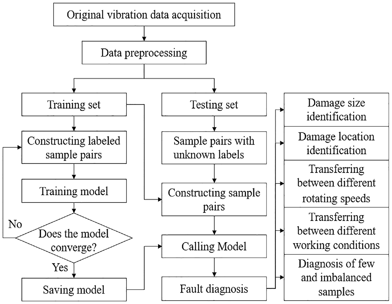
The organization of the paper.
The contribution of the method to the fault diagnosis of rolling bearings is as follows:
(1) The Siamese network architectural pattern can effectively solve the problem of small and unbalanced fault samples in the process of damage location and quantitative identification of the actual aeroengine rolling bearing, and improve the diagnosis effect of the model.
(2) The combination of meta learning and metric learning can achieve diagnosis between different rotating speeds under complex working conditions of rolling bearings, and improve the generalization ability of the model.
(3) The traditional model has a high dependence on prior knowledge of rolling bearings and insufficient feature extraction ability. However, the combination of CNN and BiLSTM can fully extract the multidimensional and temporal features of rolling bearing vibration signals to better learn the advanced features of different fault types of signals.
Siamese CNN-BiLSTM network model
Siamese net
SNs are a neural network structure for small sample learning. There are often two inputs, which are encoded by two weight-sharing neural networks of the same structure. The similarity between two inputs is output. SN-based rolling bearing fault diagnosis methods use offline-trained models to classify a new unknown fault by the similarity. In the diagnosis process, the model does not need to be updated in real time, so it is able to diagnose faults at fast speed and in real time. In addition, SNs learn by finding the similarities between two inputs with the help of two identical structures, generate labels and measure the similarities between two inputs by selecting a positive sample and a negative sample and combining them to form a sample pair. Therefore, SNs have the special advantage in small and imbalanced sample learning.
The learning principles of SNs are as follows. Firstly, two samples
The contrastive loss function was used in this study, and it is defined as:
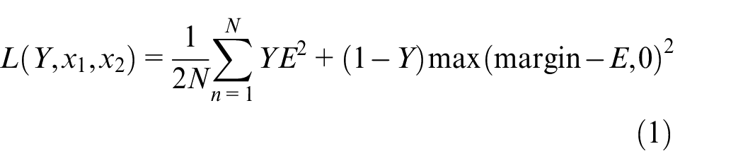
where Y is label, with a value of 1 or 0, margin is similarity threshold which is set to 1 in this paper, and E is energy function. Euclidean distance was as the energy function in this study, and it is defined as:
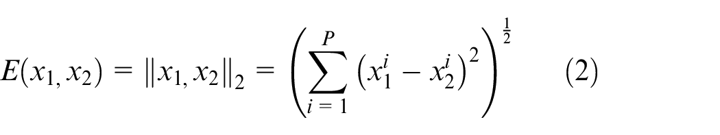
where P is the characteristic dimension.
According to Formula (1) and (2), when the samples are of different types, the energy function has a larger value, and the loss function has a smaller value, indicating these two functions can accurately describe the similarity between samples and facilitate feature extraction from samples.
Convolutional BiLSTM network model
In order to take both deep multidimensional features and temporal features of rolling bearing fault signals into consideration, the CNN-BiLSTM model was used as the feature extractor of the SN. This model is constituted by connecting a deep CNN and a BiLSTM in a series. It is able to learn deep features and temporal dynamic information of input original vibration signals of rolling bearings. The CNN can adaptively capture spatial features of bearing faults from original signals and reduce redundant data. The BiLSTM network is responsible for extracting temporal features from data. The combination of these two networks facilitates the full extraction of fault features in the circumstance of sample samples. 19
CNN
CNNs are a multilayer perceptron neural network, which can mine richer and deeper data information through weight-sharing convolution. As the most commonly used method in deep learning, deep CNNs have the advantage of automatically learning more abstract features from data. 20 The deep CNN constructed in this paper comprises an input layer, convolutional layers, pooling layers, a dropout layer, batch normalization (BN) layers, and a fully connected layer. The working principles and parameters of each layer are as follows:
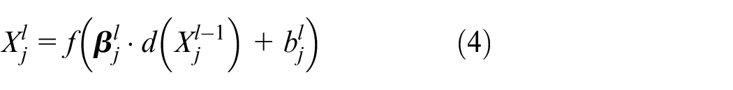
(1) Convolutional layer. Convolutional layers extract features from input images, conduct convolution computation through several convolutional kernels and input matrices, and obtain feature vectors for feature extraction through an activation function. There are three convolutional layers, each of which contains 16, 32, and 32 kernels. The activation function is ReLU. The calculation process of convolutional layers is as follows:
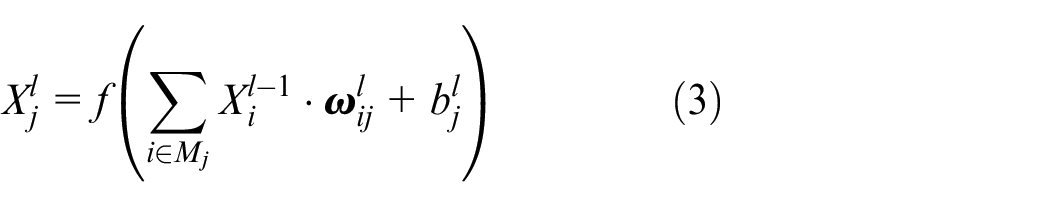
where
(2) Pooling layer. The pooling layer is used to reduce the dimension of input features, so as to improve computational speed and reduce the chance of overfitting. Three 2 * 2 average pooling layers are stacked alternately with three convolutional layers in order to reduce the dimension of data and extract features. The calculation process of pooling layers is as follows:
where
(3) Dropout layer. Neurons are randomly set to zero in a ratio of 0.2, thus preventing network overfitting and improving the generalization performance of the model. 21 The computational process of the dropout layer is:

where x. y are respectively the input and output of the layer,
(4) BN layer. A BN layer is added after the input layer and before the dropout layer, so as to accelerate network training, prevent gradient explosion or disappearance, reduce the chance of overfitting, as well as avoid the variance shift problem caused by the joint use of the dropout layer and BN layer. 22
(5) Fully connected layer. After feature extraction by the above-mentioned layers, the fully connected layer classifies features.
BiLSTM network
Although CNNs can extract abstract features of rolling bearing failures, CNNs ignore the temporal relationship between data points when they extract features from the vibration signals of bearings, which are one-dimensional temporal signals, leading to fault feature information loss in the circumstance of small samples. Thus, in this paper, the LSTM network was used to extract temporal relationships between fault features. Meanwhile, in order to take into account both forward and backward information of vibration data of rolling bearings and to improve the LSTM network’s ability to get information extract backwards, the BiLSTM network was established, which is composed of two LSTM layers of opposite directions. The forward propagation layer and the backward propagation layer propagate layer-by-layer starting from the first and last segments of the sequence, respectively. Both of them are coupled to the same output layer and share common weights, and they ultimately synchronously process the two results obtained. The BiLSTM network can integrate past and future information to further relieve information forgetting and improve prediction accuracy.
Calculations in the LSTM unit are as follows:
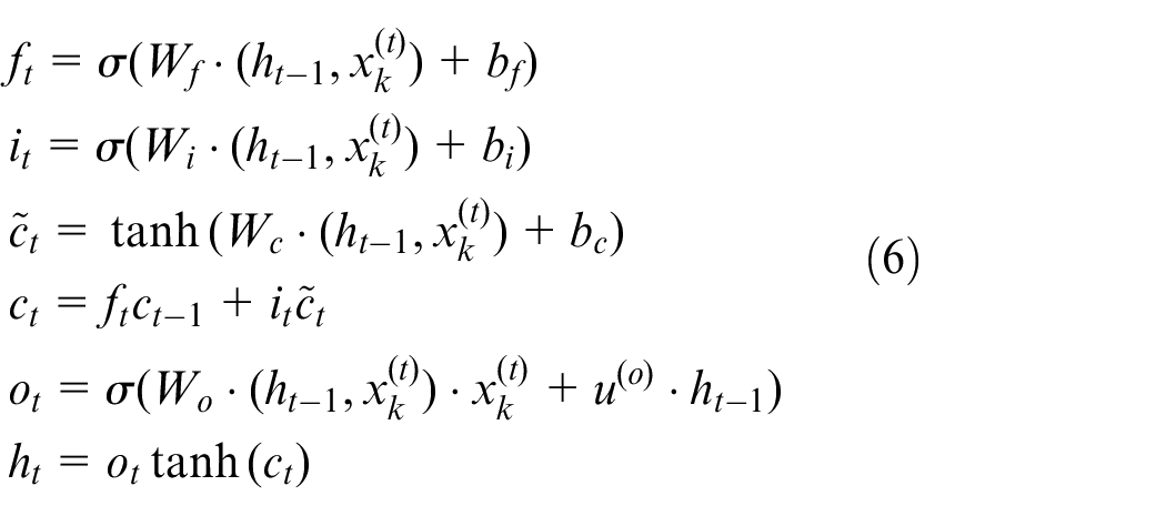
where W and b are the weight matrix and offset vector obtained through model learning, respectively;
In this paper, the CNN model was combined with the BiLSTM model. Firstly, the vibration signals of each bearing was input into the CNN model for two-dimensional feature extraction. Then, the outputs were transmitted as unit time steps to the LSTM model for temporal feature extraction. To achieve this process, the entire CNN network was enclosed in a time distribution layer so that it could be used for multiple times and deliver successively a range of extract image features to the LSTM model. The structure of the LSTM model is shown in Figure 2.
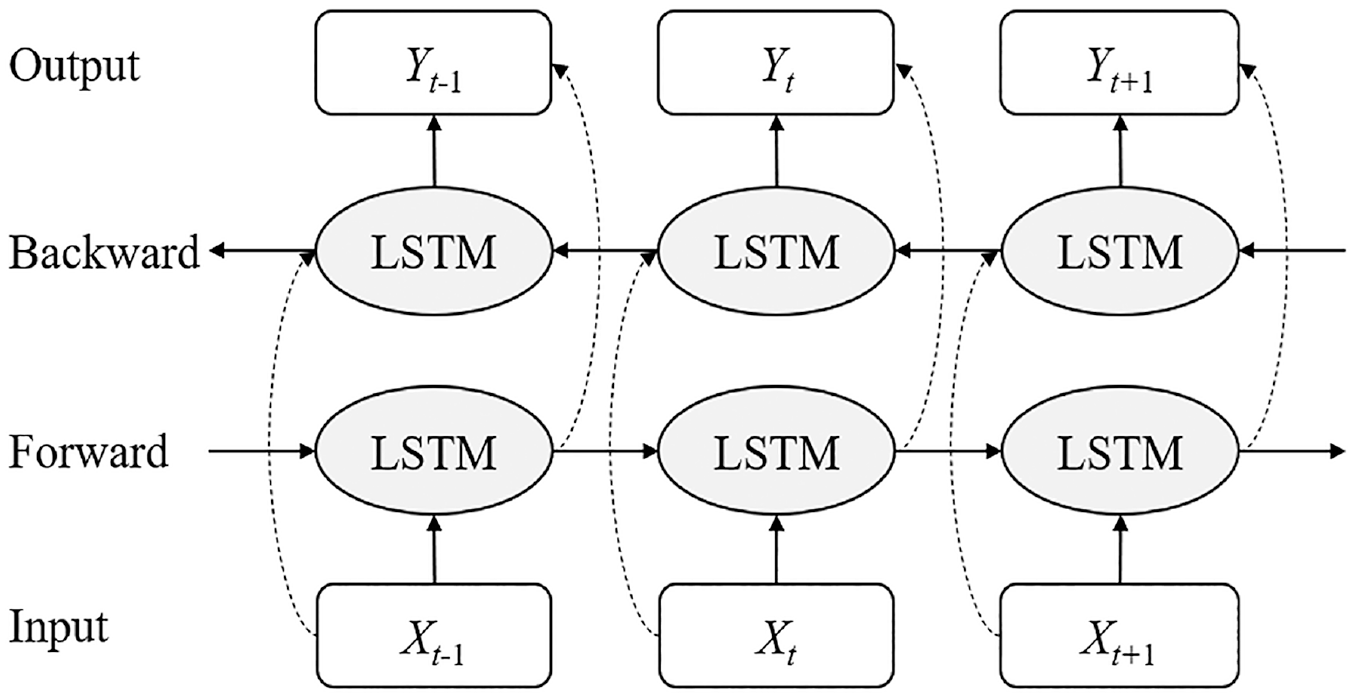
BiLSTM network structure.
Siamese CNN-BiLSTM model-based fault diagnosis of rolling bearings
Cross augmentation of data samples
The currently used methods for increasing sample size include Data Augmentation (DA) and Generative Adversarial Networks (GAN), etc.23,24 DA cannot fundamentally change the dependence on big data of the model, and is prone to generate invalid samples that are considered no difference by the network. As for GAN, the training process of which is difficult to synchronize the balance of two adversarial networks, which can easily lead to instability in the training process. In addition, GAN generates samples with a crash pattern, which makes it easy to generate meaningless samples with little difference. The combination of sample pairs achieves maximum utilization of a small number of samples, avoiding the interference of false and invalid samples on the network.
SNs select samples to form sample pairs, which are taken as the training set. Samples of the same type are labeled as positive samples, and samples of different types are labeled as negative samples. The similarities between two inputs are measured with the contrastive loss function. For a “n-way k-shot”
25
problem, a total of
Siamese CNN-BiLSTM model
To fully extract the spatial and temporal features of rolling bearing faults and quantify and locate rolling bearing damage with small and imbalanced samples, the Siamese CNN-BiLSTM model comprising two identical CNN-BiLSTM subnetworks was developed in this study. Especially, the parameter selection of CNN plays a crucial role in the performance of the model. A deeper model means better non-linear expression ability, which can fit more complex feature inputs. However, excessively deep networks may lead to gradient instability, network degradation, etc., resulting in a decrease in model performance. In order to find the most suitable network construction way, the convolutional-pooling layer is set as the basic nonlinear transformation module. By gradually deepening this module, the loss accuracy and training time of the network on the validation set are examined, and the optimal combination way is selected accordingly. The impact of different nonlinear module numbers on network loss and training speed on two sets of bearing datasets is shown in Figure 3.
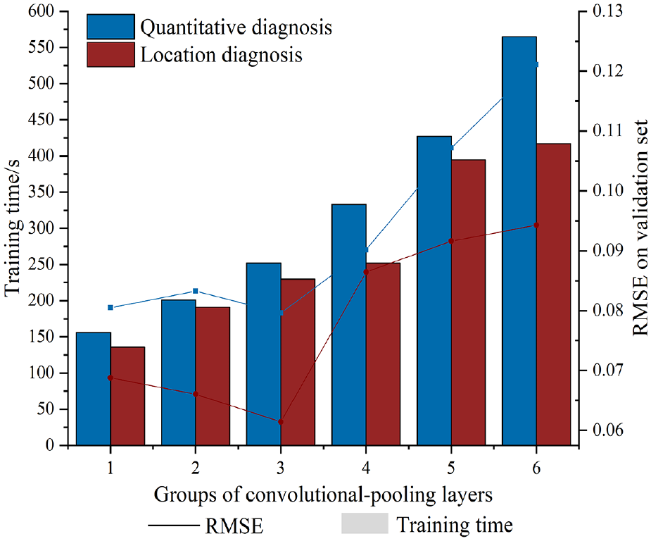
The Influence of the number of groups of convolutional-pooling layers on network performance.
From Figure 3, it can be seen that as the group of convolutional-pooling layers increases, the loss of the network on the validation set decreases significantly at the beginning, reaching its lowest point at three groups. Then, as the network depth further increases, due to the overfitting coursed by gradient instability, the loss of the network gradually increases, and the complexity of the network leads to a significant increase in training time. Therefore, the paper selects three sets of nonlinear modules to form the main part of the network, which develops a convolutional network model consisting of input layer, three convolutional layers, three pooling layers, dropout layer (p = 0.2), BN layer, fully connected layer, and regression layer. The specific internal parameters are obtained through controlling variables and comparative analysis, that is, the selected parameters minimize the training loss value of the network. The network parameters are shown in Table 1.
Network parameters of CNN-BiLSTM.
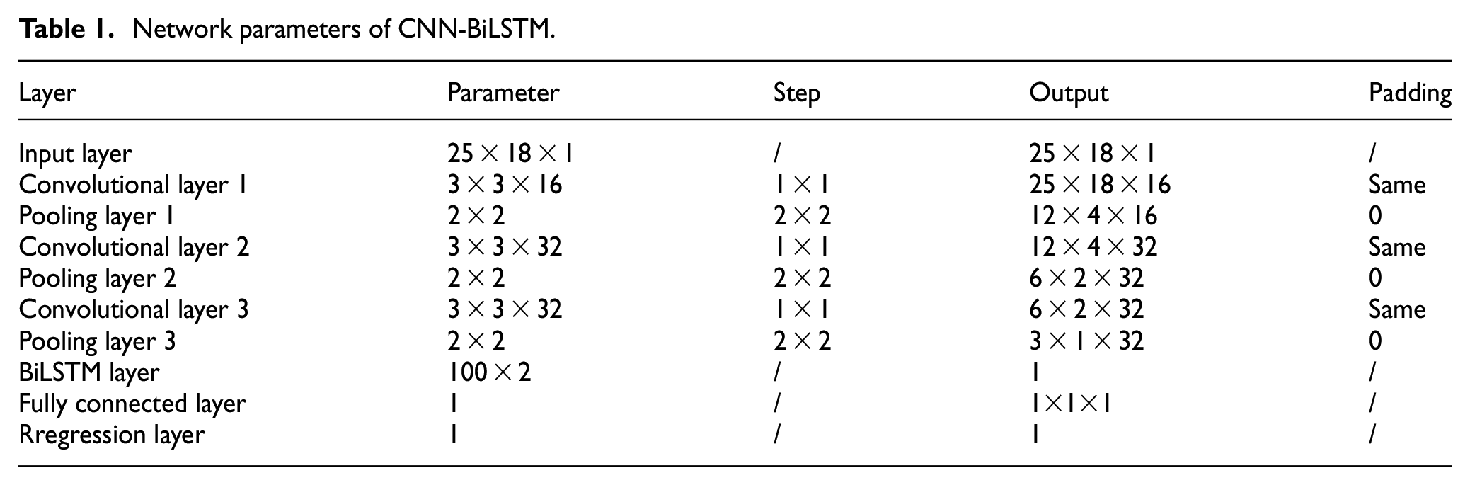
The pre-processed original signals are input into the CNN in the form of 25 × 18 × 1 matrix graphs. After three times of convolution and three times of pooling, features are unfolded and flattened, and then input into the BiLSTM network containing 200 nodes. Finally, the fully connected layer maps feature into feature vectors, and the probability of two features being similar is obtained by the activation function. Rolling bearing damage is located and quantified by comparing if the unknown sample is similar to the known sample. Feature extraction process is shown in Figure 4.
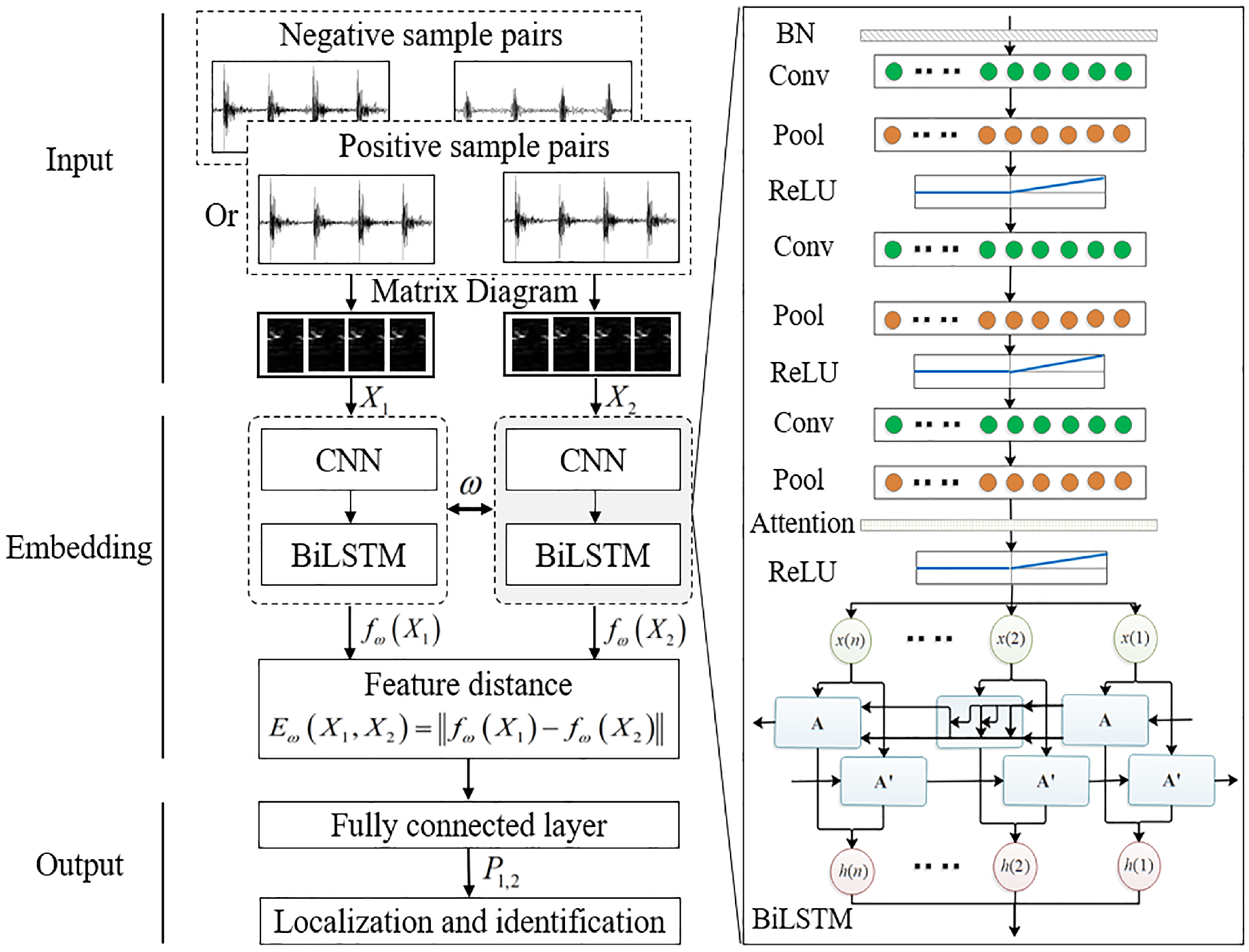
Siamese CNN-BiLSTM model-based feature extraction process.
Diagnosis process
The rolling bearing damage detection based on the Siamese CNN-BiLSTM model includes three steps below.
(1) Pre-treatment. The original vibration signal of the rolling bearing is cut into several parts according to impact peaks, and 450 points near each peak are taken as a training sample. Multiple samples are obtained from the data of each type of fault after going through the complete vibration cycle.
(2) Model training. Two samples are randomly selected from known fault samples to form a sample pair
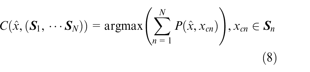
(3) Unknown fault diagnosis. Samples are selected from known fault samples to form supportive sets

For an N-class classification problem, N times of testing are required, and the supportive set is
Rolling bearing fault simulation testing
Test equipment
The test equipment used in this study is an aeroengine “rotor-rolling bearing-casing” tester, which is manufactured by a ratio of 1:3 based on a real engine model. Its overall and internal structures are shown in Figure 5. The tester has a structure similar to that of a real aeroengine. It has the same external casing as that of a real engine, but the internal structure is simplified so that effective rolling bearing vibration signals can be acquired.
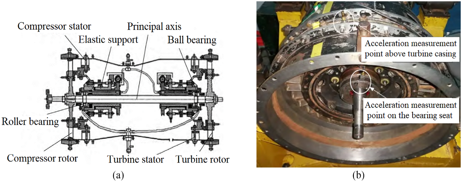
Aeroengine rotor tester: (a) overall structure and (b) internal structure.
The bearing used in the experiment is an HR6206 single row deep groove ball bearing. Pits were made on the outer race, inner race, and ball of the bearing through wire electrical discharge machining, so as to simulate faults at different sites. Meanwhile, several pits of different sizes were made on the outer raceway to simulate different sizes of faults. The picture of the rolling bearing is shown in Figure 6, and its parameters are presented in Table 2.
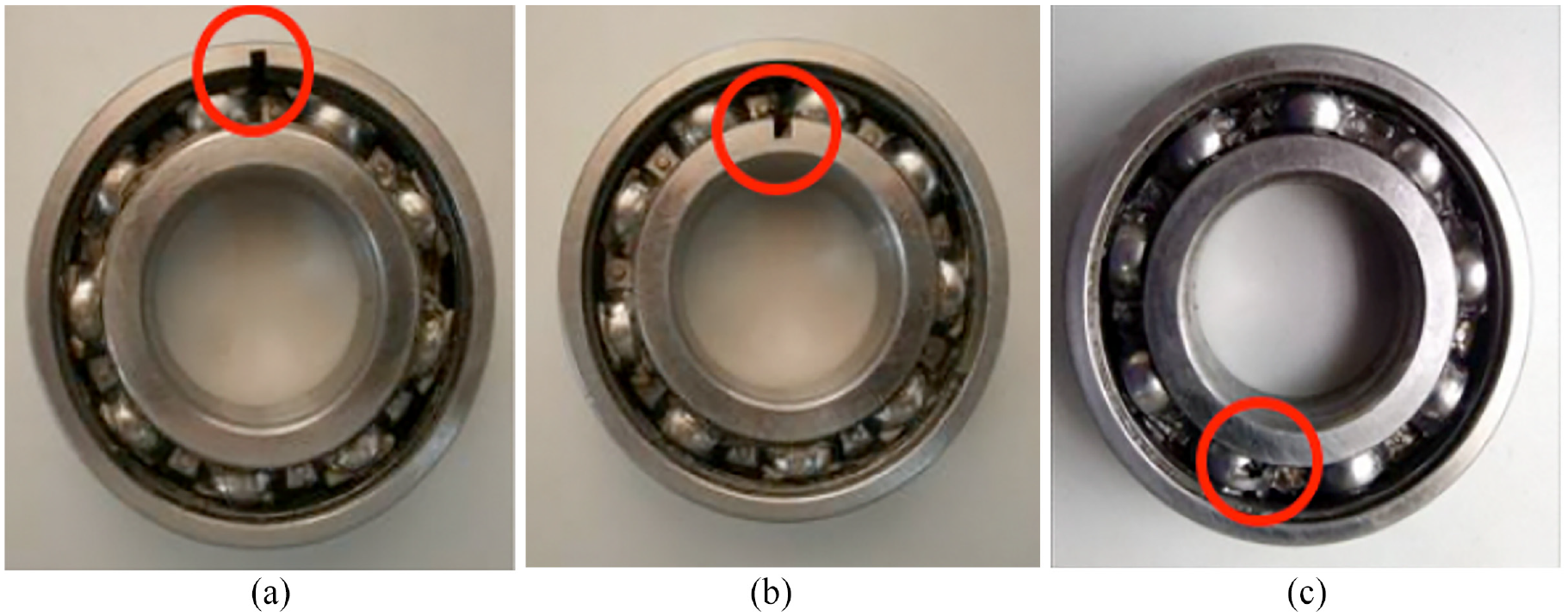
Picture of the rolling bearing after faults are made: (a) outer race fault, (b) inner race fault, and (c) ball fault.
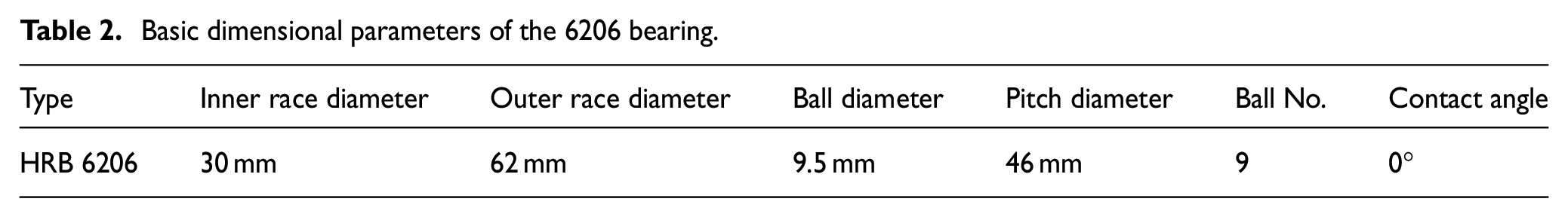
Basic dimensional parameters of the 6206 bearing.
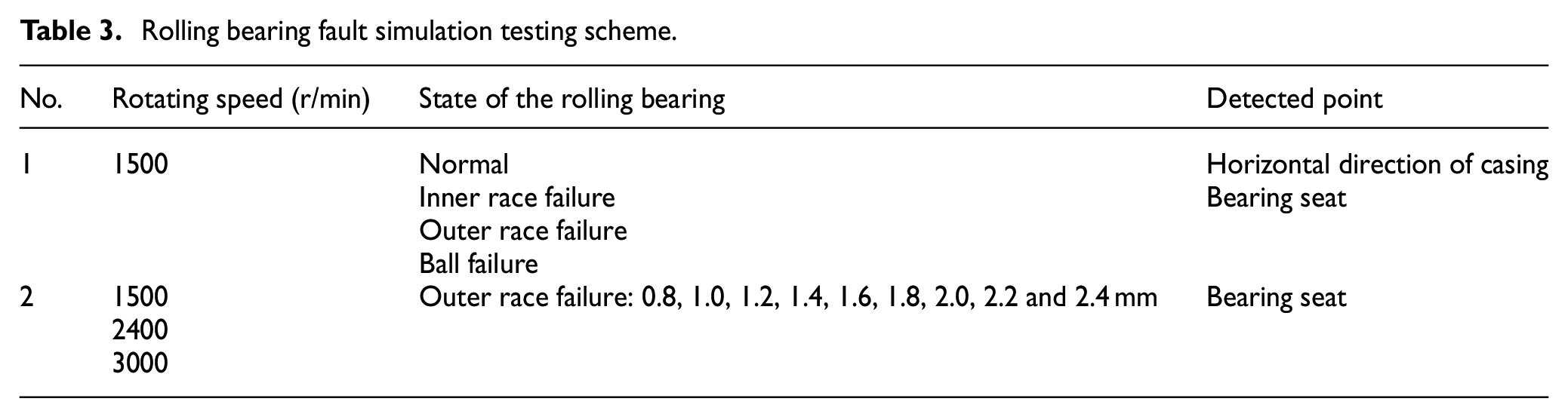
The simulation experiment is divided into two parts. On the one hand, a normal bearing, a bearing with faulty inner race, a bearing with faulty outer race, and a bearing with faulty ball were put inside the rotor tester with casing. Vibration acceleration sensors were arranged on the bearing seat and in the horizontal direction of the casing. Acceleration sensors (B&K 4805) and data acquisition boards (NI USB9234) were used to collect vibration signals and the data of damage at different sites on the rolling bearing. On the other hand, nine different sizes of penetrating grooves were made on the outer raceway of the rolling bearing by wire electrical discharge machining to simulate different sizes of spalling damage. The bearing seat was provided with B&K 4805 sensors for collection of signals and data of different sizes of damage on the rolling bearing. The sampling frequency in the experiment is 10 kHz. The experiment scheme is shown in Table 3.
Rolling bearing fault simulation testing scheme.
Experimental data
Vibration acceleration signals of rolling bearings were collected following the above-mentioned experimental scheme. Time-domain waveforms of faults of different sizes and at different locations are shown in Figures 7 and 8.
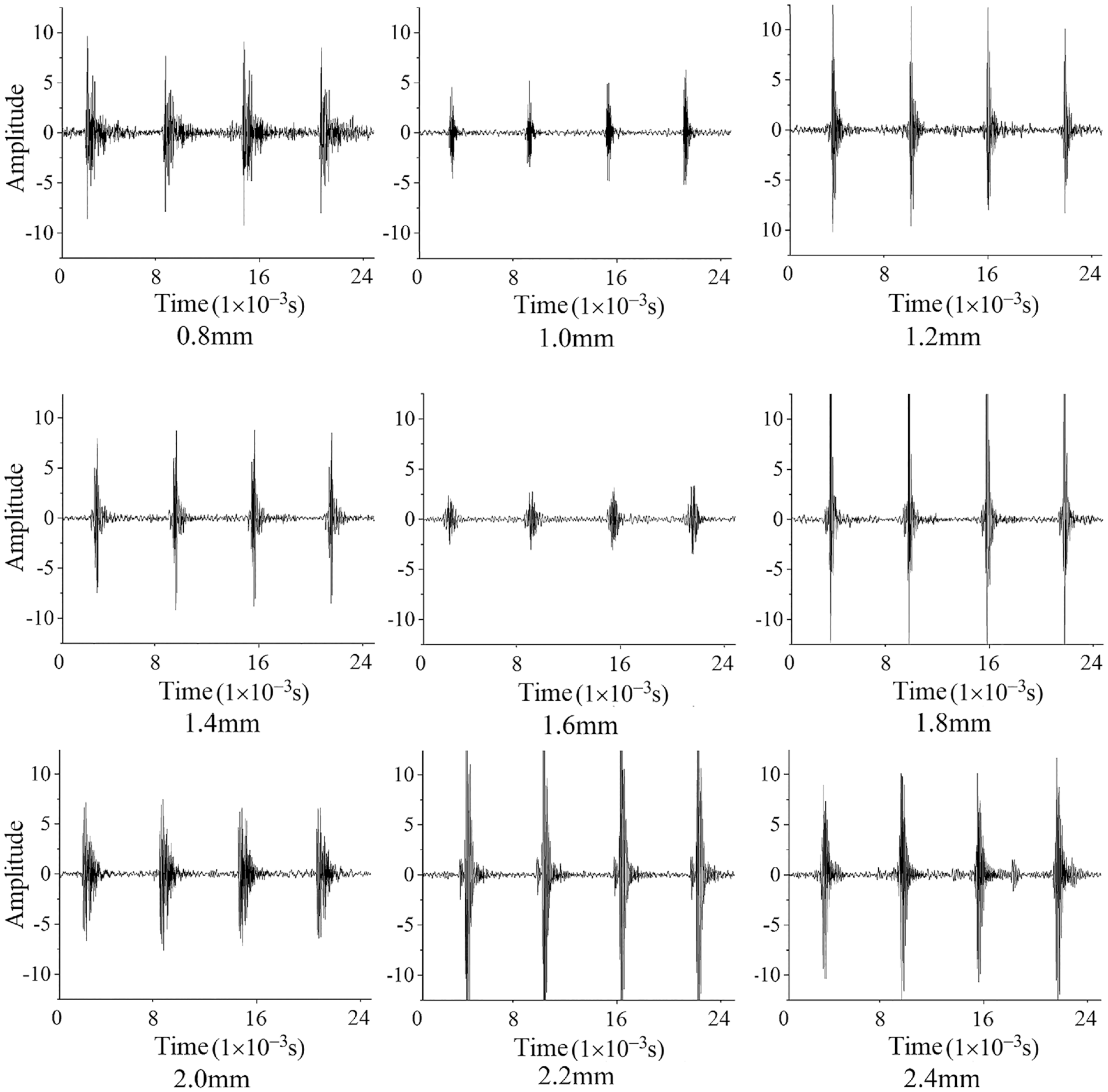
Time-domain waveforms of faults of different sizes.
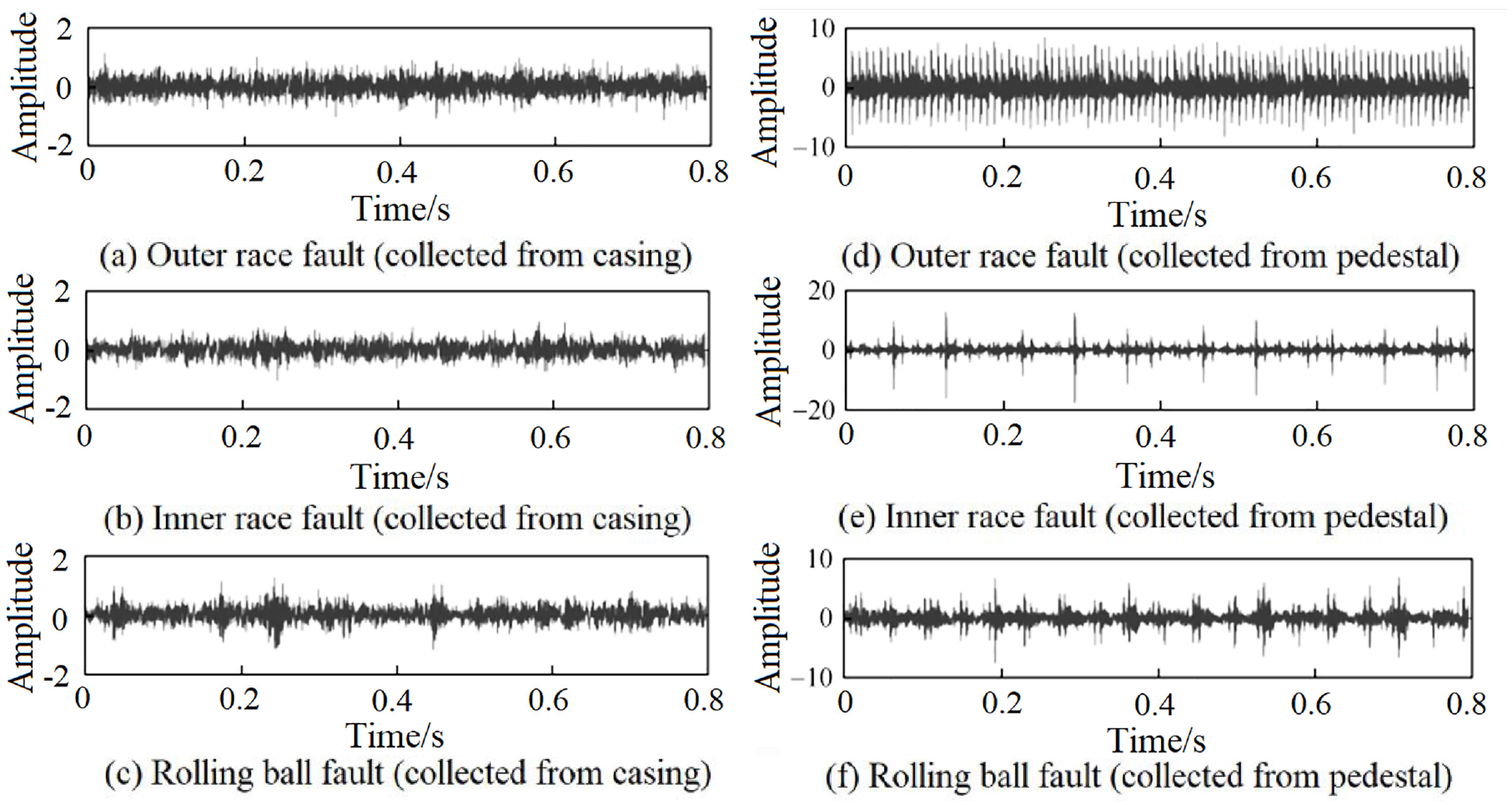
Time-domain waveforms of faults at different locations.
(1) it is impossible to determine the fault size of the rolling bearing only based on the amplitude of vibration impacts, and corresponding feature extraction models are needed to extract feature information from the temporal data in the time-domain waveforms of impact signals.
(2) Signals from the bearing seat show notable fault impact features with a high amplitude, while the impact features in signals from the casing are masked by noise, which are not evident, with an extremely low amplitude. Taken above, conventional signal processing methods cannot extract directly fault size and location information of bearings. A deep feature extraction model is needed to extract deep features hidden behind the vibration time-domain waveform and noise.
Siamese CNN-BiLSTM model-based quantitative diagnosis of rolling bearing damage
The identification of different damage sizes for rolling bearings is actually a process of considering the changes in damage over time. The trained model can identify specific damage sizes based on a small number of samples, which essence is to monitor the evolution state. In this paper, the Siamese CNN-BiLSTM model was trained with nine different sizes of faults on the rolling bearing. The samples were randomly selected and combined in order to balance and augment data. Two samples of the same class were labeled as a positive sample pair and two samples of different types were labeled as a negative sample pair. After model training, the test data and known data were input into the model as sample pairs, and whether they belong to the same class was determined based on the distance metric. In this way, the failure size was determined.
Data pre-treatment
The original vibration signals collected from the rolling bearing were pre-processed, eliminating the influence of noise while saving the essential information of fault features. This pre-treatment helps improve diagnosis accuracy. It is necessary to analyze the law and characteristics of impact signals caused by damage on the rolling bearing surface on the mechanism level. According to the studies by Randall and Sawalhi, the interval between the two impact peaks from the ball entering to leaving the spalling area is proportional to the fault size, and it can be used as a measure of the fault size.26,27 The principle is shown in Figure 9.
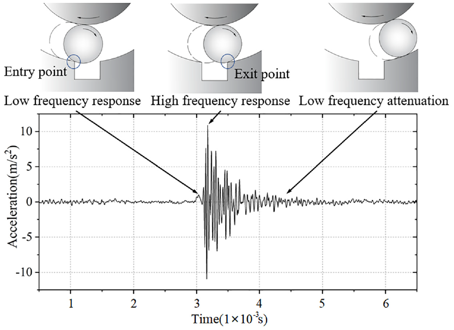
Vibration effect caused by the ball from entering to leaving the spalling area.
During data pre-treatment, vibration signals containing fault information should be saved. In this study, the peak value of the vibration signal generated by each impact was taken as the origin, and 150 points before the origin and 300 points after the origin were chosen for continuous interleaved sampling to form a 25 * 18 data matrix as a learning sample. Multiple learning samples were obtained by going through all the impact cycles of each time sequence (Figure 10). This pre-treatment method segments the original signal without doing unnecessary processing, capable of saving fault information in the vibration signal as much as possible while preventing interference by noise.
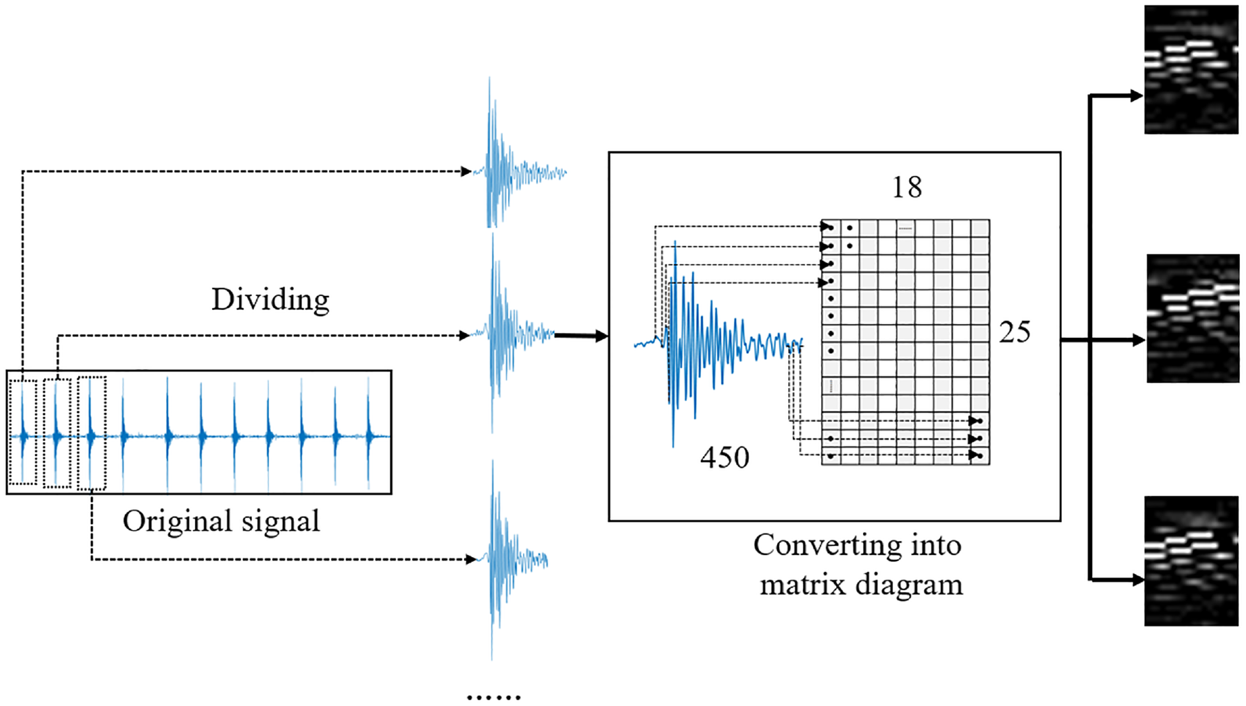
Original signal segmenting and continuous interleaved sampling.
Attention mechanism
The attention mechanism in the Transformer model 28 was introduced in this paper to promote the capture of relationship features between temporal signals. This mechanism can assign a weight to the input by itself, thereby enabling the model to focus on the essential information of rolling bearing faults and improving the efficiency of feature extraction. The process is as follows:
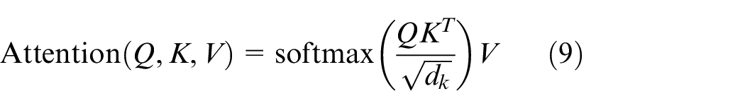
where Q, K, and V are the tested matrix, key matrix, and input data matrix, respectively; T is the time step of the input matrix, and N is the number of variables.
The attention mechanism was introduced to capture data features in this paper. The output of the last convolutional layer was activated and then up-sampled to the original image size to yield the attention activation region (Figure 11). The intensity of the color represents the size of the attention weight. Areas with a higher weight are paid more attention by the network. It can be seen from the figure that the network puts more emphasis on the area near the vibration peak, which reflects the damage size. The finding demonstrates that the network can learn the essential features of faults.
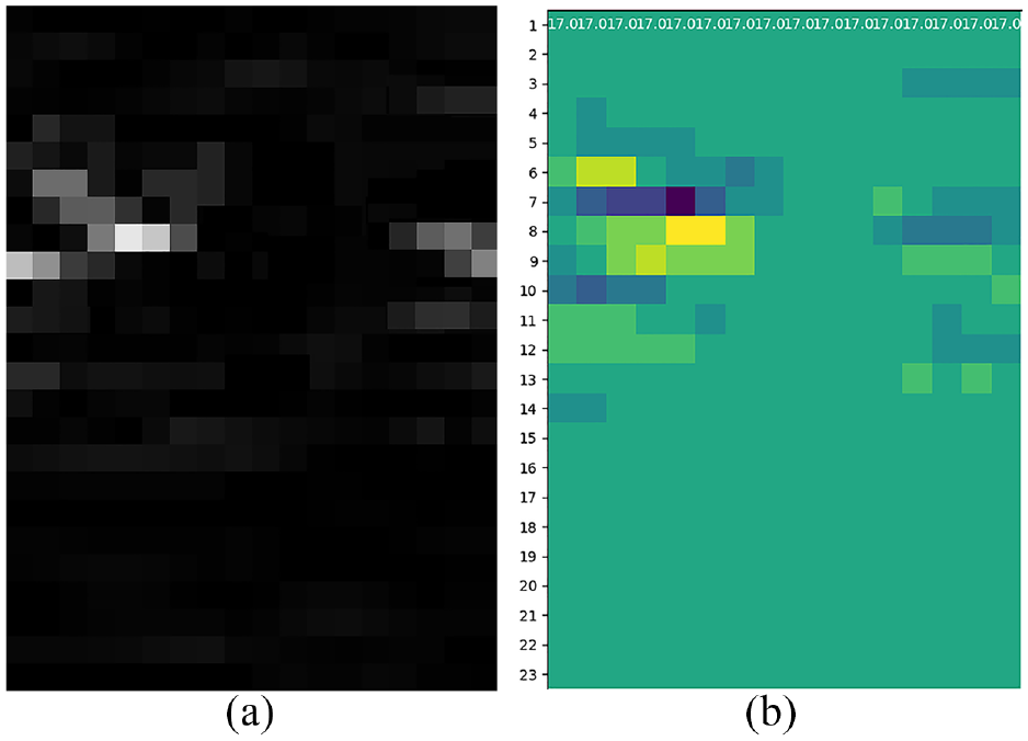
Attention mechanism: (a) original data matrix and (b) attention heatmap.
Diagnosis results
To show the classification effect vividly, the T-distributed stochastic neighbor embedding (T-SNE) method was used to visualize the features extracted from the network. This method maps each data point to the corresponding probability distribution through mapping transformation, thereby reducing the dimension of data and visualizing them. 29 The results are shown in Figure 12.
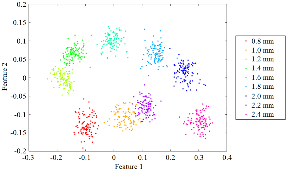
Dimension reduction results of nine-class features of the SN.
As shown in Figure 12,
(1) the Siamese CNN-BiLSTM model can well classify data of the same type into one group, thus achieving fault diagnosis with small samples.
(2) The features of faults of different sizes after dimension reduction are distributed in a certain pattern. Points with similar sizes are closer in distance, demonstrating that the Siamese CNN-BiLSTM model can classify data based on distance measurement and adaptively learn the damage pattern of rolling bearings.
SNs have special advantages in small sample learning as they are trained with samples obtained by random selection and combination methods and learn similarity metrics. To further investigate the effect of the sample size on the performance of the network, the classification accuracy of the Siamese CNN-BiLSTM model was examined with different sizes of training samples. The number of training samples increases while the number of testing samples remains 100. The results are shown in Figure 13.
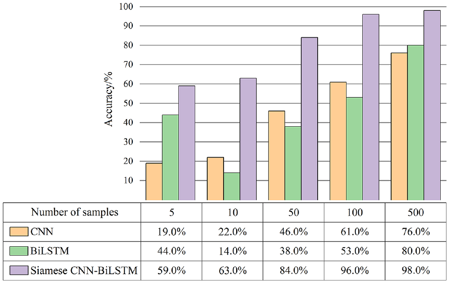
Effects of the sample size on the accuracy of the network (2400 r/min).
It can be seen from Figure 13,
(1) CNN, BiLSTM and Siamese CNN-BiLSTM models all have a low diagnosis accuracy when there are extremely few samples. With the increase in the number of samples, the models get more training and their accuracy increases gradually.
(2) Compared with CNN and BiLSTM models, the Siamese CNN-BiLSTM model has a higher accuracy in various circumstances of small samples, indicating its superiority in diagnosis with small samples.
Transferring between different rotating speeds
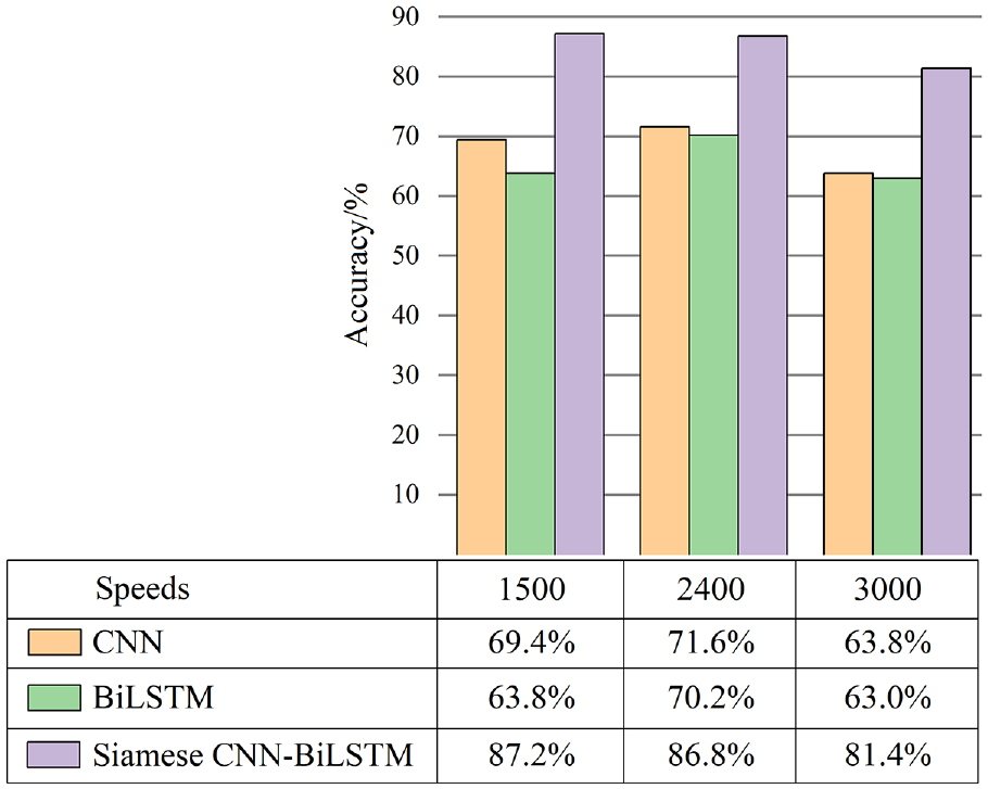
As the rotating speed of the rotor changes, the vibration signal of the rolling bearing alters significantly, directly weakening the diagnosis performance of the deep learning model. The generalization performance of models at different rotating speeds (A: 1500 r/min, B: 2400 r/min, and C: 3000 r/min) was studied, and their transfer accuracies between different rotating speeds were analyzed. The number of testing samples is 500. The diagnosis accuracies of models transferring between different rotating speeds are shown in Figure 14.
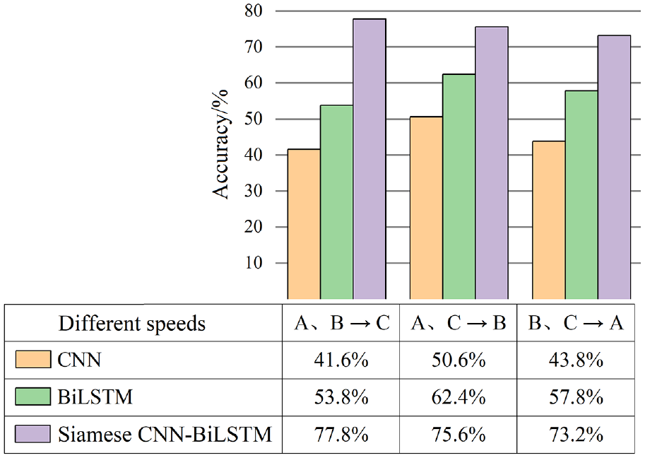
Effects of transferring between different rotating speeds on the accuracy of the network.
When the rotating speed begins to change, the diagnosis accuracy of both CNN and BiLSTM models decreases markedly. However, the average diagnosis accuracy of the Siamese CNN-BiLSTM model is 39.98% and 23.21% higher than that of CNN and BiLSTM models, respectively. It proves the good generalization performance of the Siamese CNN-BiLSTM model.
Siamese CNN-BiLSTM model-based location diagnosis of damage
Diagnosis results
The Siamese CNN-BiLSTM model was used to classify four types of faults and locate the fault on the rolling bearing. The classification results after T-SNE visualization are shown in Figure 15. It can be seen that the Siamese CNN-BiLSTM model can better locate the failure on the rolling bearing.
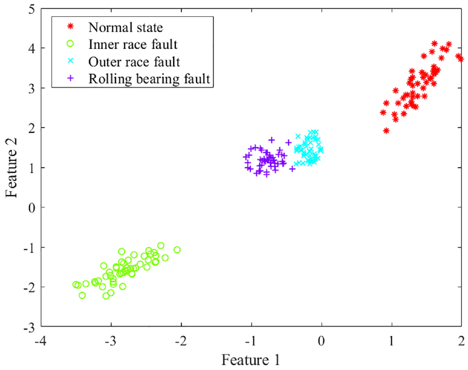
Dimension reduction results of 4-class features of the SN.
Transferring in complex working conditions
The vibration signals of real aeroengines in service are generally gathered by sensors provided on the casing wall. In experimental environments, however, sensors are often installed on the bearing seat for data collection. There are some differences in feature distribution between the two conditions. Thus, models trained with the data collected from the bearing seat are often not applicable to the analysis of the data collected from the casing wall. It indicates the model lacks the generalization ability. In this study, the Siamese CNN-BiLSTM model was trained with the data collected from the bearing seat and its accuracy was verified with the casing dataset. The accuracy of the Siamese CNN-BiLSTM model was compared with that of conventional single models, and the results are shown in Figure 16.
Effects of transferring between different working conditions on the accuracy of the network.
According to the comparison results, CNN and BiLSTM models trained with bearing seat signals have relatively lower performance on the casing dataset. In contrast, the Siamese CNN-BiLSTM model has a higher transfer accuracy, demonstrating that the model has better generalization performance and can transfer between different working conditions to some extent.
Siamese CNN-BiLSTM model-based diagnosis with small and imbalanced samples
Due to its unique structure and training method, the SN has special advantages over conventional single deep neural networks in solving the problems of small and imbalanced samples. To demonstrate the superiority of the SN in diagnosis with small and imbalanced samples, a unilateral Siamese CNN-BiLSTM model was employed in this paper, which was trained by traditional loss optimization methods, namely, forward input and reverse iteration. Moreover, the damage diagnosis results of the SN were compared with those of conventional networks based on the data of damage at four different sites on the rolling bearing.
Results of diagnosis with small samples
The Siamese CNN-BiLSTM model and single CNN-BiLSTM model were used to locate the damage at four different sites on the rolling bearing. The training and testing sets contain only 50 samples for each type. The damage location results are compared in Figure 17.
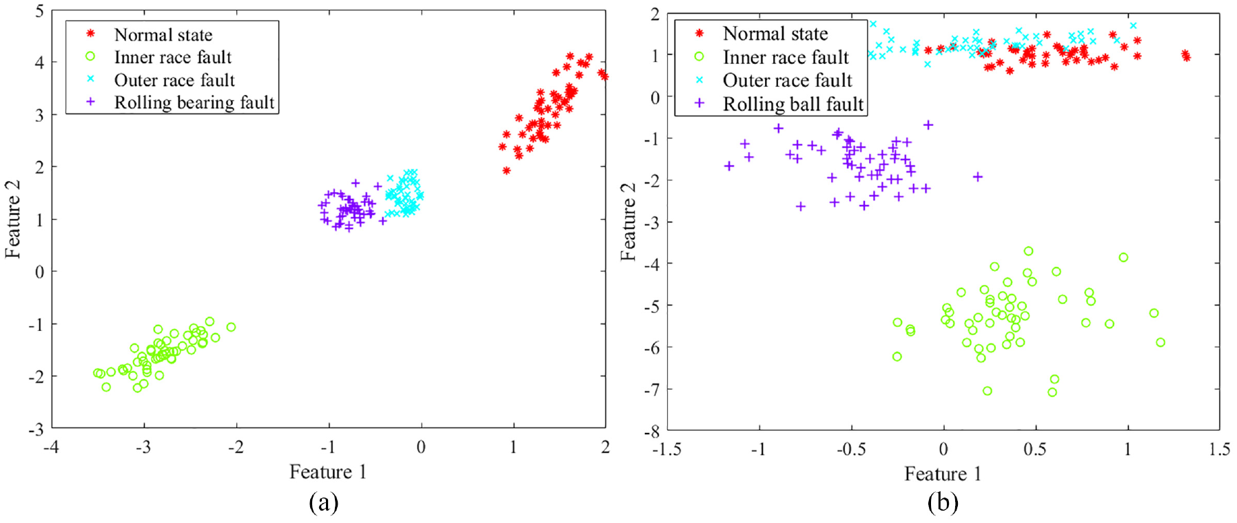
Results of location diagnosis of damage at four different sites with small samples: (a) Siamese CNN-BiLSTM and (b) CNN-BiLSTM.
As shown in Figure 17, after dimension reduction, the fault features predicted by the single CNN-BiLSTM model show a high overlap ratio, indicating that this model cannot locate the damage at four different sites on the rolling bearing. The reason is that the small number of samples makes it difficult for the model to converge. In other words, the model fails to learn fault features and is thus underfitting. However, after embedding a weight-sharing Siamese structure into the same single CNN-BiLSTM model, a high accuracy was achieved. The reason is that through cross pairing and metric learning, the SN has strong generalization ability even when there is a small number of samples, and meanwhile, the chance of overfitting is greatly reduced.
Results of diagnosis with imbalanced samples
The inputs of common neural networks are various types of untreated samples. In contrast, during the training of the SN, samples are selected from the original data and combined to form Siamese pairs before being input into the embedding module for feature extraction. This process breaks the original classification relationships, allowing the original samples to be presented in the form of new sample pairs. Hence, it balances the number of different types of samples. To sufficiently compare the performance between the SN and common networks in solving the problem of sample imbalance, CNN-BiLSTM and Siamese CNN-BiLSTM models were used to classify the imbalanced data of damage at four different locations. There were 50 normal data, 30 inner and outer ring fault data, and 10 ball fault data. The classification results are shown in Figure 18.
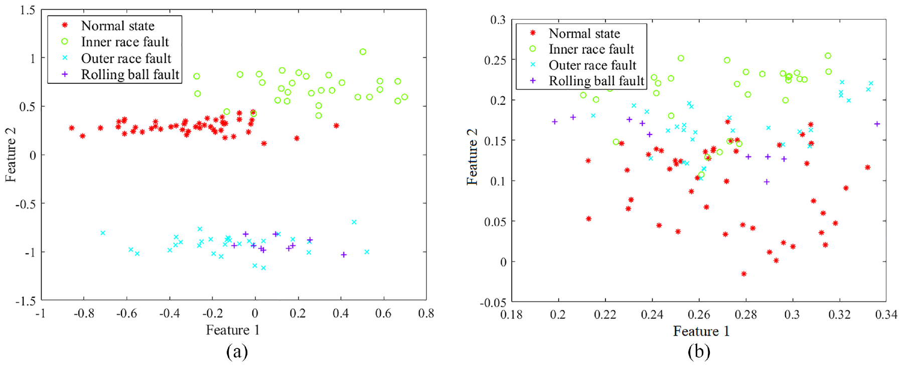
Results of location diagnosis of damage at four different sites with imbalanced samples: (a) Siamese CNN-BiLSTM and (b) CNN-BiLSTM.
According to Figure 18, different types of samples contribute disproportionally to the gradient of the conventional single model when the number of samples of different types is unequal, and the model pays more attention to the type containing more samples during predication. As a result, the model fails to learn the essential features of the fault. The SN model, however, balances the classes by selecting sample pairs, and thus achieves a higher diagnosis accuracy for imbalanced samples.
Conclusion
A Siamese CNN-BiLSTM model was proposed to locate and quantify the aeroengine rolling bearing damage with small and imbalanced samples. After multiple experimental comparisons, the following conclusions are drawn.
(1) When there are only 100 samples in the training set, the Siamese CNN-BiLSTM model achieves an accuracy of 96.0% for quantifying and 98.0% for locating rolling bearing faults. This model is capable of effectively diagnosing faults with small samples.
(2) The Siamese CNN-BiLSTM model enables the rolling bearing to transfer between different rotating speeds and different working conditions. Compared with conventional single models, the Siamese CNN-BiLSTM model has a high transfer accuracy, demonstrating that it has better generalization performance.
(3) The SN can balance the number of samples through the combination of sample pairs, so it is more accurate in diagnosis than the CNN-BiLSTM model.
The reason for the above results lies in the two major advantages of Siamese network: metric learning ideas and sample pair extraction and concatenation, combined with the superiority of CNN-BiLSTM in feature extraction of rolling bearing vibration time series signals, making it well adapted to the fault diagnosis problem of rolling bearing with a small number of imbalanced samples. However, Siamese network also has certain limitations. Firstly, although it can achieve data expansion through sample recombination and comparison, at the same time, the way of sequential comparison also reduces recognition speed; In addition, we have demonstrated through experiments that the Siamese network has higher accuracy in the aspect of unbalanced fault diagnosis with few samples compared with the ordinary network, but it can be seen from the text that the fault diagnosis accuracy is only about 80% when the number of samples is relatively small, which has improved the diagnosis of actual rolling bearing faults, but still insufficient enough. Further research and exploration are needed on how to improve the diagnostic ability of small sample networks and make them more suitable for real service conditions.
Footnotes
Declaration of conflicting interests
The author(s) declared no potential conflicts of interest with respect to the research, authorship, and/or publication of this article.
Funding
The author(s) disclosed receipt of the following financial support for the research, authorship, and/or publication of this article: This research is sponsored by National Science and Technology Major Project of China (J2019-IV-004-0071) and National Natural Science Foundation of China (52272436).