
Abstract
Aiming at the problem of fault diagnosis and classification of rolling bearing and gear of gearboxes, a novel method based on matrix distance features of Gramian angular field (GAF) image is proposed based on sliding window compressible GAF transformation. The method converts the one-dimensional fault signal into a two-dimensional feature matrix and constructs the discrimination matrix of each fault category by establishing the mean value of the feature matrix of a priori samples. For the new sampled signal, after converting it into a two-dimensional feature matrix, the feature matrix is obtained. The fault classification is carried out by using the matrix distance between feature matrix and the discrimination matrix of each category. The method is validated by the test data of Case Western Reserve University and the acoustic emission data from a gearbox test bench. The classification accuracy is 99.17% and 95.71%, which presented the feasibility and effectiveness of the novel method proposed in this paper.
Introduction
Gearbox is an important component of mechanical equipment, which is widely used in the field of mechanical engineering, and the occurrence of gearbox failure will directly affect the normal operation of the whole mechanical equipment, so its condition monitoring and fault diagnosis not only have theoretical research significance but also practical application value.1–3 In most fault diagnosis, it is a common method to use vibration signal to monitor the condition of rotating machinery. The fault of gearbox generally occurs in bearings and gears, and the vibration signals usually was accompanied by strong background noise and modulated of fault impact components, so it is difficult to diagnose the fault directly.
For the characteristics of gearbox fault signals, the commonly used methods for gearbox fault diagnosis mainly include time-frequency analysis methods,4–6 feature extraction classification,7–9 and neural network classification.10–12 For example, Faysal et al. 13 proposed an improved method named noise eliminated ensemble empirical modal decomposition (NEEEMD) method that further reduces the white noise in the eigenfunction and keeps the system optimal overall, which can identify more fault feature pulses from the envelope spectrum and can be used as a more accurate rotor bearing fault diagnosis system. 13 Guo et al. 14 proposed a method based on optimized wavelet packet denoising (WPD) and modulated signal bispectrum (MSB) fault diagnosis scheme, which utilizes the transient pulse enhancement of WPD and the demodulation capability of MSB to diagnose bearing faults more accurately and has a better effect on suppressing strong background noise and interference components. 14 Jiao et al. 15 proposed a new bearing fault feature extraction method that combines multiscale sample entropy (M-SSampEn) with energy moment (EM) to construct the energy moment (M-SSampEn-EM) feature extractor based on time-domain multiscale sample entropy, and experiments showed that the classifier has better generalization performance for bearing fault classification. 15 Song et al. 16 proposed a new bearing diagnosis method based on the decomposition of vibration signals using the empirical wavelet transform (EWT) with adaptive empirical mode segmentation and the merging of redundant empirical modes. 16 Liu et al. 17 proposed a new algorithm for bearing fault diagnosis by combining multi-scale one-dimensional convolutional neural network (1-D CNN) with sparse wavelet decomposition feature extraction. 17 Meng et al. 18 proposed a rolling bearing fault diagnosis method based on multiscale combined morphological filter (MCMF) and self-adaptive improved multiscale fuzzy entropy (SAIMFE), and the experimental results show that the method not only has high diagnostic accuracy but also has less dependence on the diagnostic model. 18 For the rolling bearing vibration signal is a typical non-smooth signal, Sun et al. 19 proposed a new fault diagnosis method based on the improved Manhattan distance in Symmetrized Dot Pattern (SDP) image. 19 In order to solve the problem that rolling bearings have too many characteristic parameters with remarkable randomness and severe signal coupling during operation, Zhou et al. 20 proposed a new bearing fault diagnosis method by combining Gramian angular field (GAF) and dense network. 20 Zhu et al. 21 transformed bearing fault diagnosis into a class of pattern classification problems and proposed an intelligent fault diagnosis method based on principal component analysis (PCA) and deep Belief Network (DBN). 21 In order to solve the unclear fault characterization of rolling bearing vibration signal due to its nonlinear and nonstationary characteristics, Zhou et al. proposed a rolling bearing fault diagnosis method based on whale gray wolf optimization algorithm variational model decomposition-support vector machine (WGWOA-VMD-SVM). 22
Although the above methods have achieved the target of fault diagnosis, there are still some shortcomings. Some methods lack comprehensive data reconstruction when preprocessing the original signal, which disrupts the temporal correlation of the data and leads to information loss. In addition, the applicability of some feature extraction methods is limited, they only have a good effect on the target fault diagnosis, and the corresponding effect is not achieved in other fault diagnosis methods. According to the characteristics of gearbox fault signals and the advantages of GAF conversion to ensure the time correlation of signals, a fault diagnosis method based on matrix distance features of GAF images is proposed in this paper. This method not only adopts the GAF method to ensure the temporal continuity of the signal, but also proposes a feature extraction and classification method with wider adaptability, simpler, and higher accuracy based on Euclidean distance features. The main process of this method is to use empirical mode decomposition to extract the IMF component with the largest kurtosis value to achieve noise reduction. Then the envelope demodulation of the signal after noise reduction is carried out, and the upper envelope signal is extracted as the processed signal. Next, the Piecewise aggregation approximation (PAA) method is used to down-sample the processed signal. The one-dimensional data is converted to two-dimensional space by the Gramian angular summation field (GASF) method, and the average distribution matrix of priori samples is calculated as the discriminant matrix for fault classification. When using PAA for down-sampling, it is necessary to select a suitable sliding window to compress the data to reduce the amount of calculation. Finally, the distance between the sample and the discriminant matrix is calculated as the similarity evaluation index to realize the fault classification of the sample.
Basic principle
Empirical modal decomposition
Empirical modal decomposition (EMD) is a time-frequency domain signal processing method that decomposes the signal based on the time-scale characteristics of the data itself. It separates the signal layer by layer according to the characteristics of different scales to generate a series of intrinsic mode function components (IMF). 23 EMD has obvious advantages in processing non-stationary and non-linear data, and is suitable for analyzing non-linear non-stationary signal sequences with high signal-to-noise ratio. The IMF component needs to satisfy two constraints.
One is that the number of extreme value points and the number of over zero points must be equal or not more than one difference. The other is that the mean value of the upper and lower envelope of the function from the maximum value and the minimum value is 0.
The whole EMD process is basically as follows.
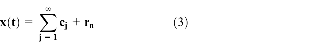
Firstly, all the pole values of the original vibration signal x(t) are found. By using a cubic spline function, the maximum point and the minimum point are connected respectively to obtain the upper and lower envelope of the vibration signal. Then the mean value

The intermediate signal

Then
EMD can decompose the original fault signal into multiple IMF components, and the effective fault signal components are concentrated in specific IMF components. By screening the suitable and effective IMF components, the interference of the noise signal can be reduced and the signal-to-noise ratio of the fault signal can be improved.
Kurtosis
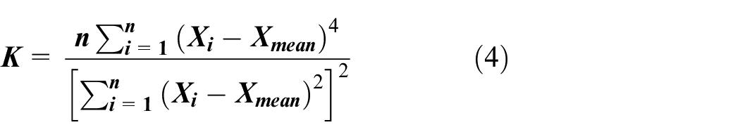
Kurtosis is a dimensionless parameter, which is a statistical parameter used to describe the peak of the waveform and is also one of the most commonly used parameters in the early fault diagnosis of rolling bearing, which can be used to characterize the size of impact in the rolling bearing fault signal.24,25 If the rolling bearing is in smooth operation and has no obvious periodic disturbance state, the probability density of its vibration signal is close to the normal distribution, and the kurtosis coefficient of the normal distribution is about
The calculation formula for the Kurtosis is listed as follows:
where
Because kurtosis has the characteristics of describing the impact strength in the signal, kurtosis index is used to evaluate each IMF component after EMD decomposition. The IMF component with strong impact contains more fault impact components. The IMF component with strong impact is selected as the processed signal, so as to realize the noise reduction of fault signal.
Envelope demodulation
If the bearing is damaged or defective, its operation will produce a damped pulse impact force, which will cause high-frequency inherent vibration of the bearing. These high-frequency vibrations will be used as the carrier waveform of bearing vibration, and its amplitude will be modulated by the pulse excitation force caused by these defects, so that the measured bearing vibration signal will show a complex modulated waveform. Therefore, it is necessary to demodulate the bearing fault signal during diagnostic analysis, and the envelope curve and envelope spectrum of the modulated signal obtained by demodulation analysis tend to carry more useful information centrally.26,27
For the analysis of bearing fault signals, the demodulation process can be performed to extract the envelope curves and thus achieve the effect of noise reduction. The envelope extraction of the signal can be performed by Hilbert method.
The specific steps of the Hilbert method are as follows:
Firstly, the Hilbert transform of
Then it is summed with

Finally, the upper envelope of the original signal

where
Gramian angular field
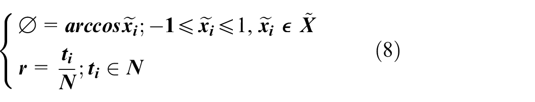
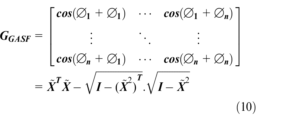
In the process of gearbox operation, the bearing vibration signal is periodic. Random noise is easy to affect the periodic vibration signal, so it is difficult to extract the bearing fault characteristics directly from the time domain signal. Gramian angular field (GAF) can realize a projection transformation of a one-dimensional signal into two-dimensional space, separate the feature signal from the interference signal, and maintain the time correlation in the transformation, and highlight the time fluctuation characteristics of the signal.
The whole steps are as follows:
Firstly, give a time series
where
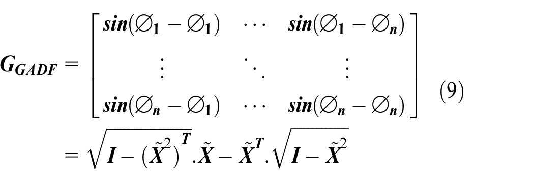
where I is the unit row vector;
The GAF method maps one-dimensional signal to two-dimensional data space. During the mapping process, the impact features of the one-dimensional signal are highlighted in the two-dimensional data space, and the temporal relationships of the signal are effectively preserved, so that the impact components in the fault signal can be more effectively expressed and displayed, which is beneficial to the subsequent fault classification.
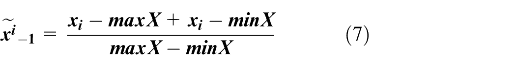
If the time series data is too long, the storage space of the device will not only have high requirements, but also consume a lot of computing time. In order to solve this problem, the Piecewise aggregation approximation (PAA) is used to realize the down-sampling of the original time series data, which can reduce the storage requirement of equipment and greatly improve the operation speed.
PAA is an effective down-sampling method that plays a significant role in reducing data storage and improving computational efficiency.
28
The data downscaling of time series is achieved by transforming a sequence
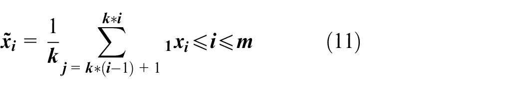
In order to achieve the purpose of data down-sampling, a compressible sliding window is used to segment the sequence X and calculate the mean of each segment, so that the data length is reduced to the original 1/k. Since the data down-sampling will lose part of the time series information, it is necessary to select an appropriate sliding window width parameter k, and reduce the amount of data computation as much as possible on the premise of ensuring accuracy.
Matrix distance similarity evaluation
The similarity evaluation of matrices is to evaluate the similarity of two matrices by calculating the metric quantity, which is equivalent to calculating the distance of two matrices. Since the general distance calculation is performed for vectors, in order to calculate the distance of two matrices, we perform the Euclidean distance calculation for the corresponding row vectors of the two matrices based on the vector Euclidean distance, and use the sum of the distance vectors as the distance indicator of the two matrices, which is calculated as described below.
Suppose there are two matrices with the same dimension and the size is
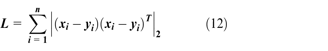
where
The distance between two matrices is visually represented by the distance metric
The steps of the proposed method
According to the above theoretical basis, this paper proposes a fault classification method which transforms one-dimensional fault signals into two-dimensional space for feature extraction.
Firstly, the two-dimensional mapping process of a single fault signal is as follows:
EMD is used to decompose the original sampled signal;
Extract the IMF component with the largest kurtosis value as the signal after noise reduction, and demodulate its envelope to obtain the envelope;
Select a sliding window of appropriate size to perform PAA down-sampling operation on the envelope signal to reduce the amount of calculation in the later stage;
The down-sampled signal is mapped to the two-dimensional space by GAF conversion to obtain its two-dimensional feature matrix.
The process steps are shown in the following Figure 1.
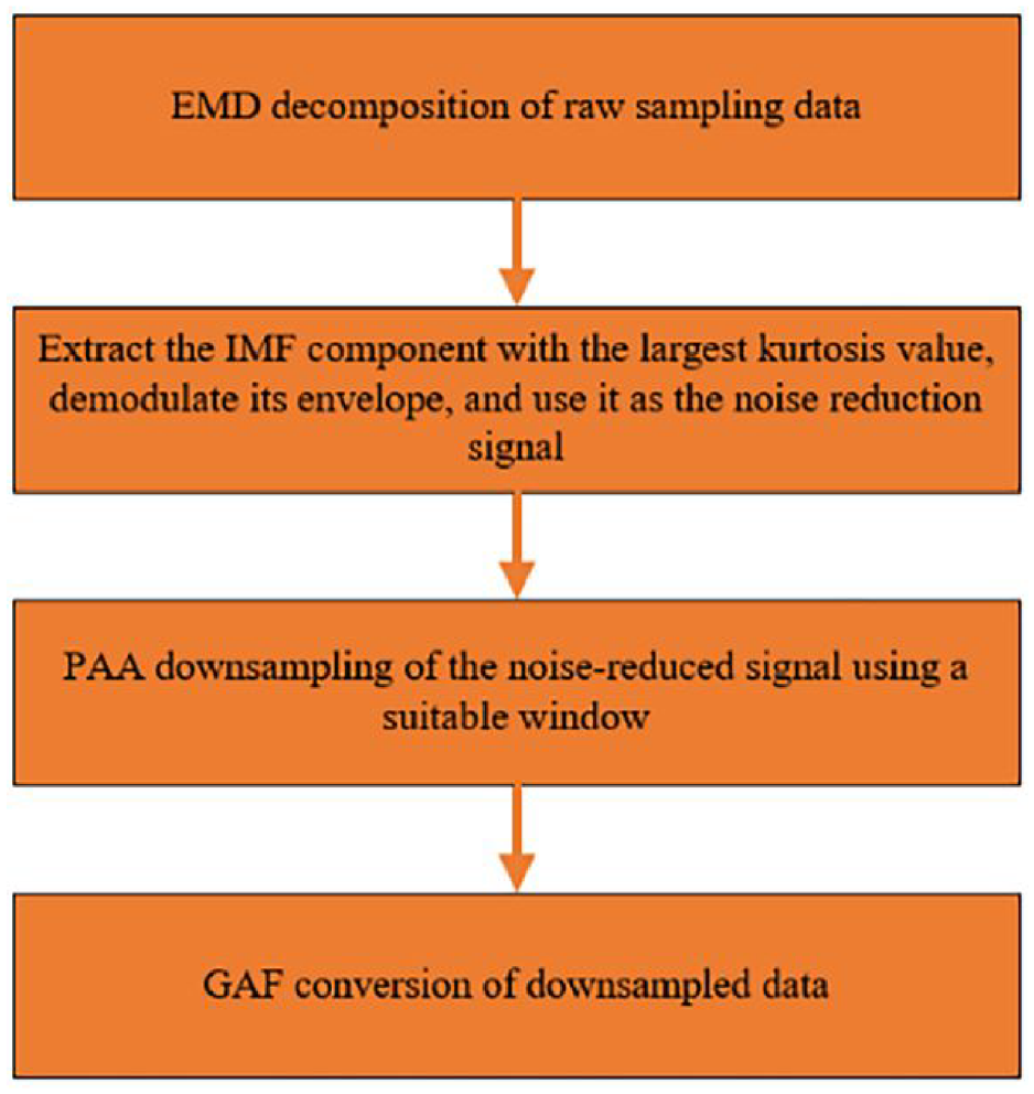
Flow chart of two-dimensional mapping.
Secondly, according to the construction of multiple samples, considering the length of the sample data, the original sampled signal can be segmented, which can extract the impact characteristics in the signal more effectively.
The specific process is as follows:
Select
Divide each signal into
For
Average
Average
Using the same processing method for different categories of data, the discriminant matrix of each category can be obtained separately.
The process steps are shown in the following Figure 2.
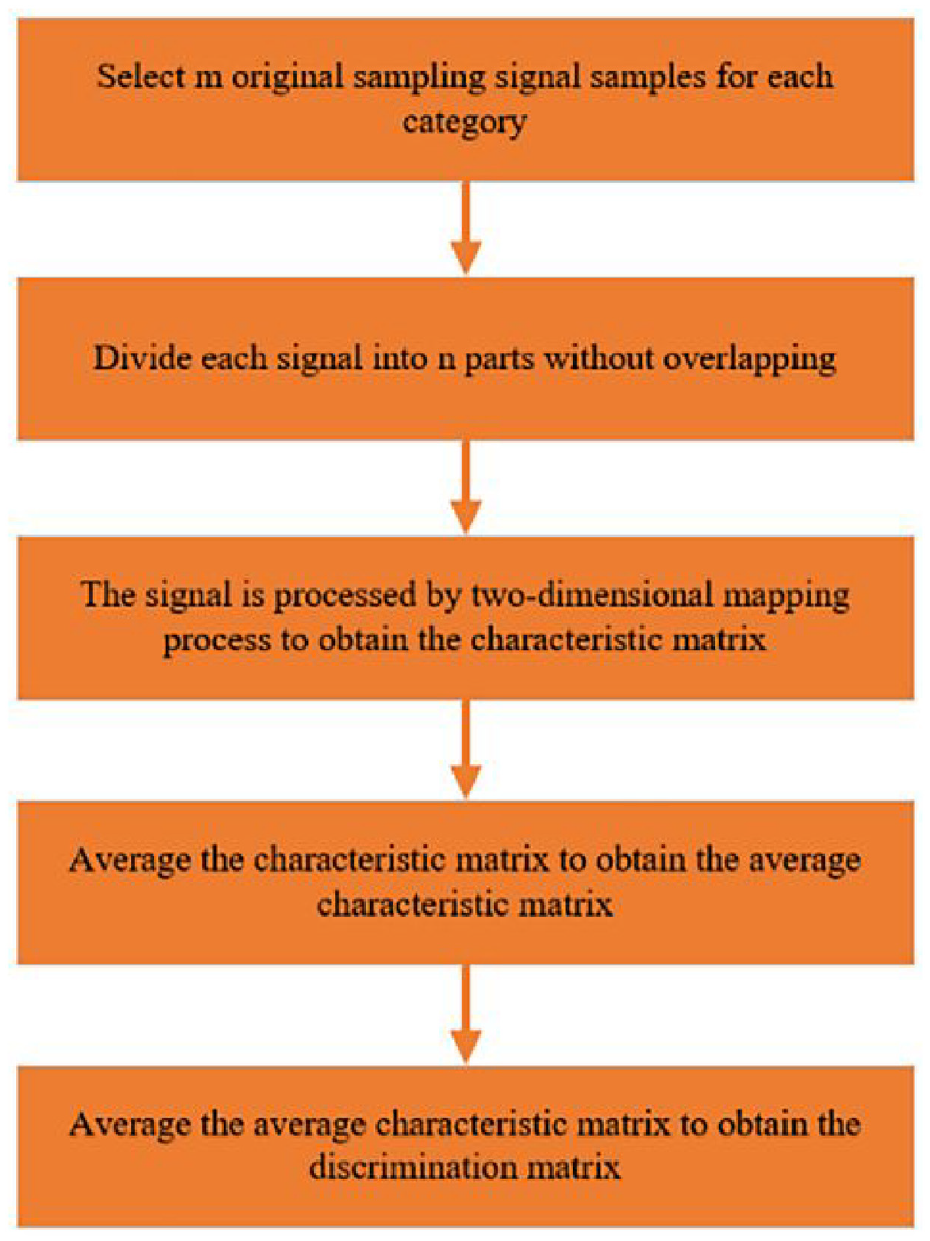
Flow chart of discriminant matrix construction.
Thus, the construction of the discriminant matrix is realized, and the discriminant matrix can be used in the subsequent fault classification detection of the measured signal.
Finally, the two-dimensional feature matrix of the test signal is calculated through the two-dimensional mapping process of a single fault signal, the matrix distance between the two-dimensional feature matrix of the test sample and the discriminant matrix of each fault class is calculated, and the category is determined according to the minimum value of the matrix distance.
The specific process is as follows:
Divide the new test samples into
For
Take the average of
According to the above equation (12), calculate the matrix distance between the feature matrix of the measured sample and the
Fault classification of the new test sample is realized. The process steps are shown in the following Figure 3.

Flow chart of fault classification and detection of test samples.
According to the previous description, the overall algorithm flow of integrating the construction of the fault classification matrix and the fault classification of the new test sample is shown in Figure 4.
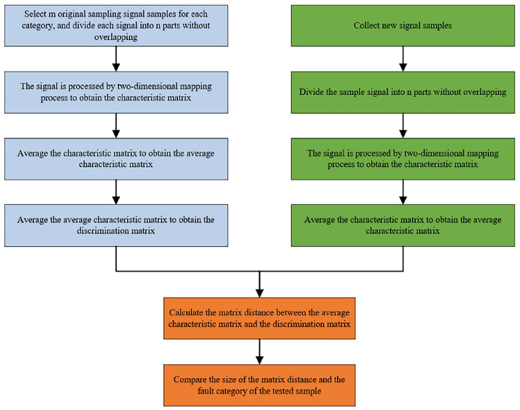
Fusion flow chart of matrix distance feature-based gearbox fault diagnosis method.
Simulation experiment
Experimental data validation
Experimental data sources
The experimental data used in this paper are all from the Case Western Reserve University Bearing Data Center (http://csegroups.case.edu/bearingdatacenter) published online. Its bearing test-bed consists of a 2-HP motor, a torque sensor/ decoder, and a power tester. The type of rolling bearing used is 6205-2RS JEM SKF deep groove ball bearing and it is placed on the motor drive end. The simulated experimental bench is shown in Figure 5. The data selected in this paper are the drive end bearing data under sampling frequency of 12 kHz, motor speed of 1750 r/min and damage diameter of 0.1778 mm, and four data sets of normal operating conditions, inner ring fault, outer ring fault at 12 o’clock, and ball fault are used.
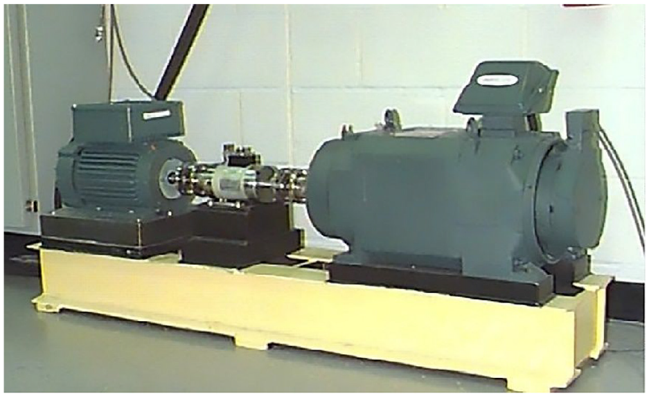
Bearing failure simulation test bench.
Specific implementation mode
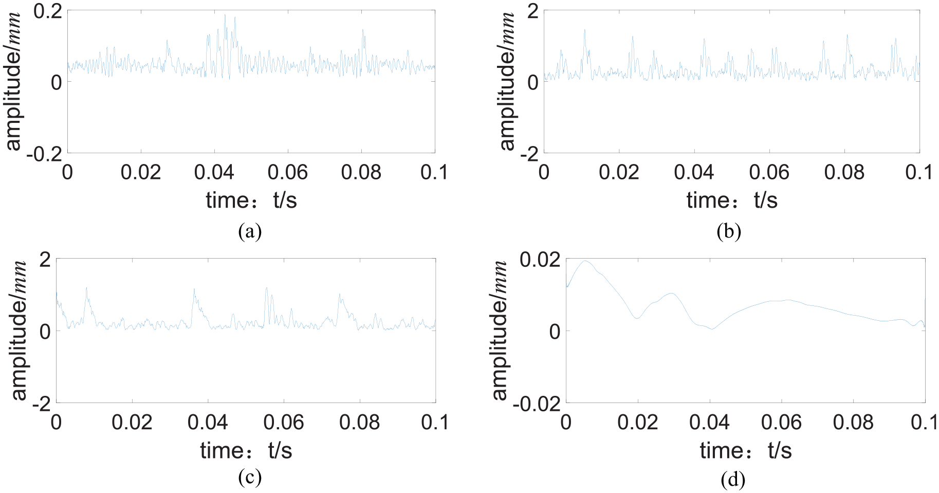
In order to ensure the sufficiency of fault information, it is necessary to select appropriate sample data length. However, due to the limited total length of data, 10 groups of sample data are selected under the normal working condition of rolling bearing, inner ring fault, outer ring fault and rolling element fault to ensure sufficient sample size, and 10 groups of sample data are selected for each state. The amount of data extracted for each group is 12,000. Each group of sample data is divided into 10 equal pieces on average, each sample data size is 1200. The time domain diagram of each group of original signals in four different categories is shown in Figure 6.
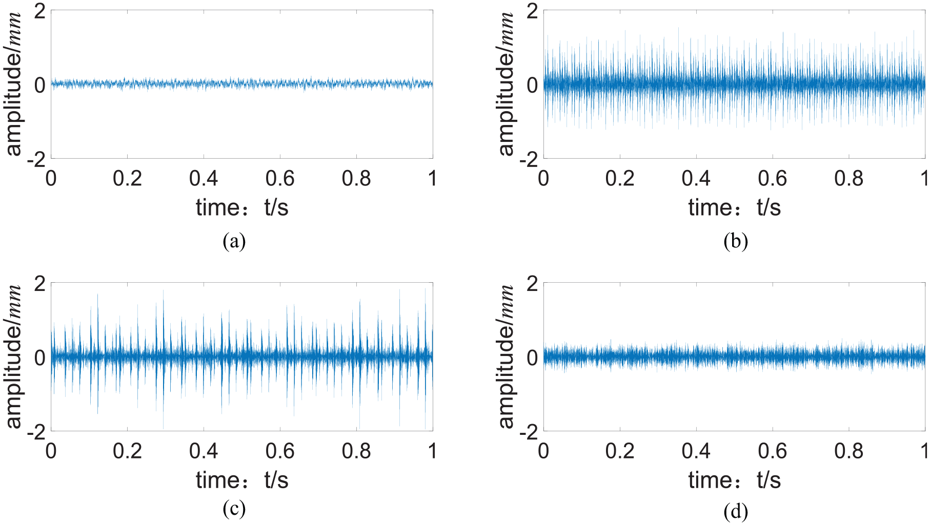
Time domain diagram of the signal for different categories: (a) normal state, (b) inner ring fault, (c) outer ring fault, and (d) ball fault.
According to equations (1)–(3), EMD is performed on the sample data to obtain multiple eigenmode components. The time-domain diagram of IMF components in each category is shown in Figure 7.
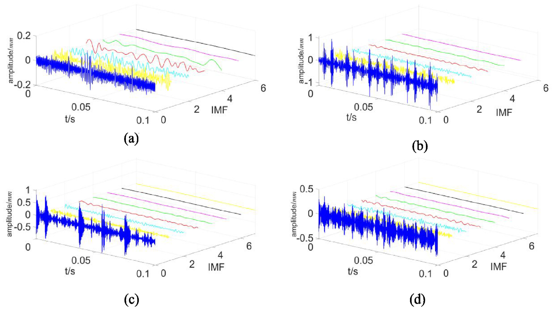
IMF component after EMD decomposition for different categories: (a) normal state, (b) inner ring fault, (c) outer ring fault, and (d) ball fault.
According to equation (4), calculate the kurtosis values of each IMF component in different categories, and the results are shown in Figure 8.
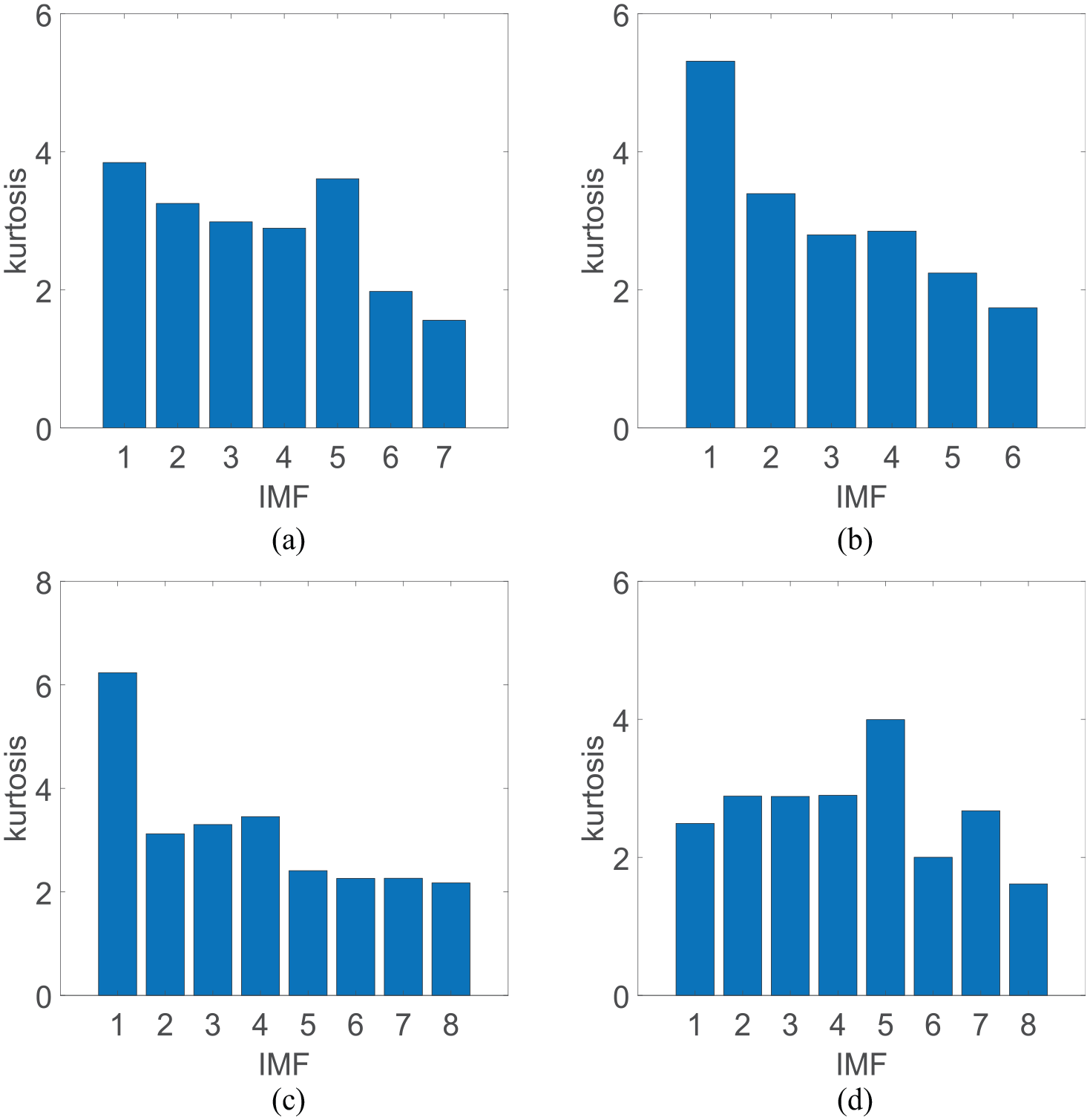
IMF component kurtosis values for different categories: (a) normal state, (b) inner ring fault, (c) outer ring fault, and (d) ball fault.
According to the characteristic that the larger the kurtosis value of IMF component, the more fault information it contains, the IMF component with the largest kurtosis value is selected as the denoising signal. The time domain diagrams of the IMF signals with the largest kurtosis values in the four different categories are shown in Figure 9.
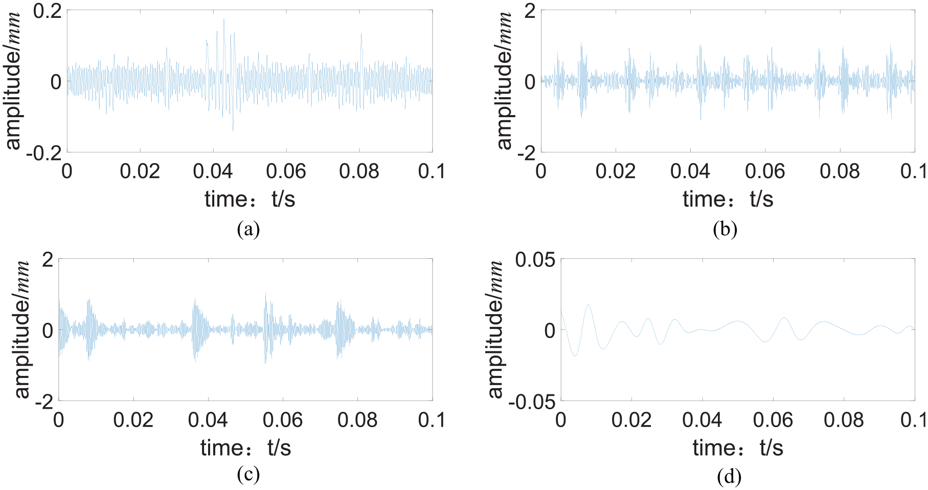
Time domain plot of maximum IMF component of steepness values for different categories: (a) normal state, (b) inner ring fault, (c) outer ring fault, and (d) ball fault.
According to equations (5) and (6), the IMF component with the largest kurtosis value is demodulated, and the upper envelope curve is selected as the signal for subsequent processing. The time domain plots of the upper envelope curves for the four different categories are shown in Figure 10.
The upper envelope of the IMF component with the largest value of kurtosis in different categories: (a) normal state, (b) inner ring fault, (c) outer ring fault, and (d) ball fault.
After analysis, the effect of signal fault impact components after using the GASF method is more obvious, so the GASF method has a better effect. According to equations (7), (8), (10), and (11), GASF transformation is performed on the processed upper envelope information. Before the GASF conversion of the processed signal, the PAA method can be used to select the suitable sliding window size to compress the data and reduce the amount of data calculation. Through analysis, when the sliding window size is 2, the data processing effect is better. Finally, two-dimensional feature matrices of four different states with a size of 600 × 600 are obtained, and their corresponding GASF images are shown in Figure 11.
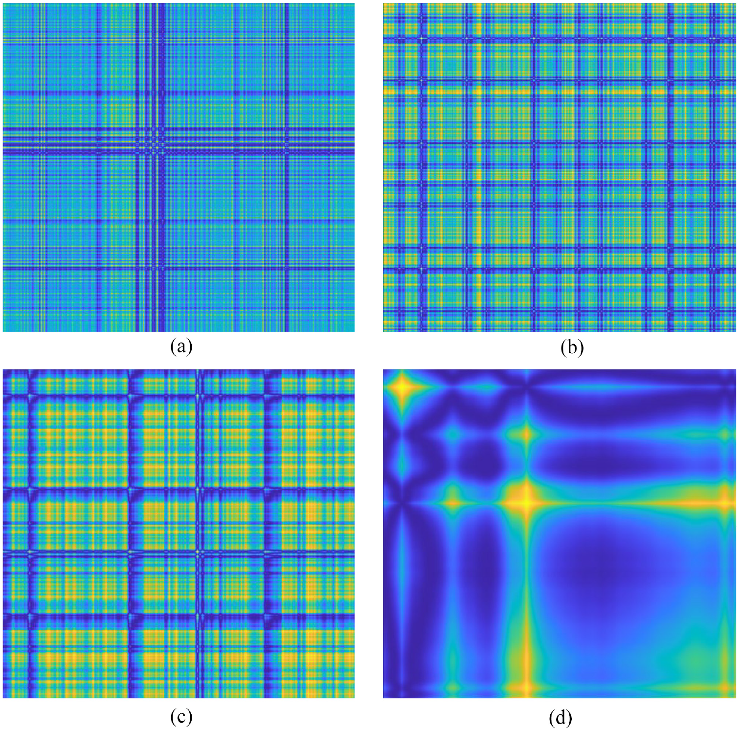
GASF images for different categories: (a) normal state, (b) inner ring fault, (c) outer ring fault, and (d) ball fault.
According to the GASF images, the corresponding 10 two-dimensional feature matrices can be obtained, and then the GASF image feature matrix corresponding to each group of sample data is obtained by averaging these 10 two-dimensional feature matrices.
According to the GASF image feature matrices corresponding to the 10 groups of sample data in different states, the average matrix is calculated to obtain the discriminant matrix of size 600 × 600 in four different states, and their GASF images are shown in Figure 12.
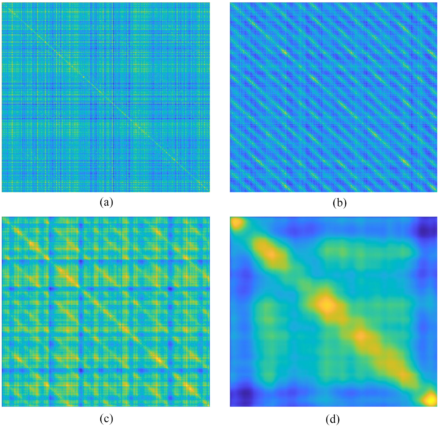
GASF discriminant matrix image for different categories: (a) normal state, (b) inner ring fault, (c) outer ring fault, and (d) ball fault.
According to equation (11), the matrix distance of GASF image feature matrix and discriminant image matrix of four different categories for each group of data is calculated.
The matrix distance between the feature matrix of the test data and the discriminant matrix in four different categories is represented by a histogram. Figures 13 to 16 show the histogram of matrix distance between the feature matrix of the test data and the discriminant matrix in four different categories respectively.
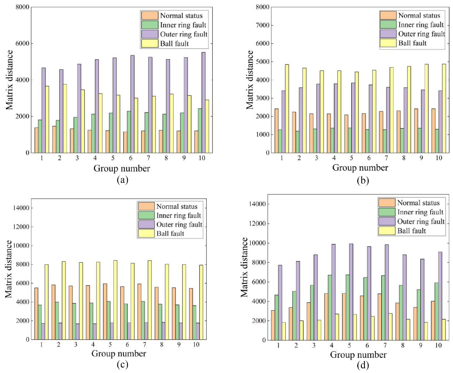
Matrix distance histogram for different categories: (a) normal state, (b) inner ring fault, (c) outer ring fault, and (d) ball fault.
Acoustic emission signal test bench.
GASF discriminant matrix images of different categories of the acoustic emission signal: (a) normal state, (b) inner ring fault, (c) outer ring fault, and (d) broken tooth fault.
Number of errors under different sliding windows.
From these histograms, it can be seen that the matrix distance between the feature matrix of each test data and the corresponding state’s discrimination matrix is smaller than that of the discrimination matrix in other states, which further verifies the effectiveness of the method.
In order to further verify the method, 90 test data groups of each state are randomly selected under the premise of not exceeding the experimental data amount, and a total of 360 test data samples are extracted. According to the above steps, the matrix distance corresponding to the average matrix of each group of data and the discriminant matrix of four different states is calculated, and the category with the smallest matrix distance is selected as the fault classification result. In the end, the overall classification accuracy of 360 test data is 99.17%.
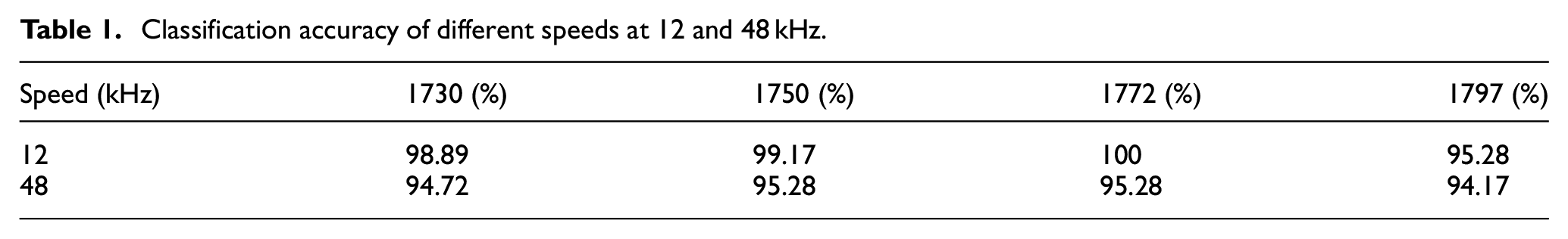
Under the same basic conditions, the vibration signals of other speeds (1730, 1772, and 1797 rpm) and sampling frequency (12 and 48 kHz) are processed in the same way. The final fault classification accuracy is shown in Table 1.
Classification accuracy of different speeds at 12 and 48 kHz.
Experimental verification of gearbox acoustic emission data
Gearbox acoustic emission data sources
In order to verify the performance of the method, the acoustic emission signal measured by a motor-driven gearbox test bench is processed and verified.
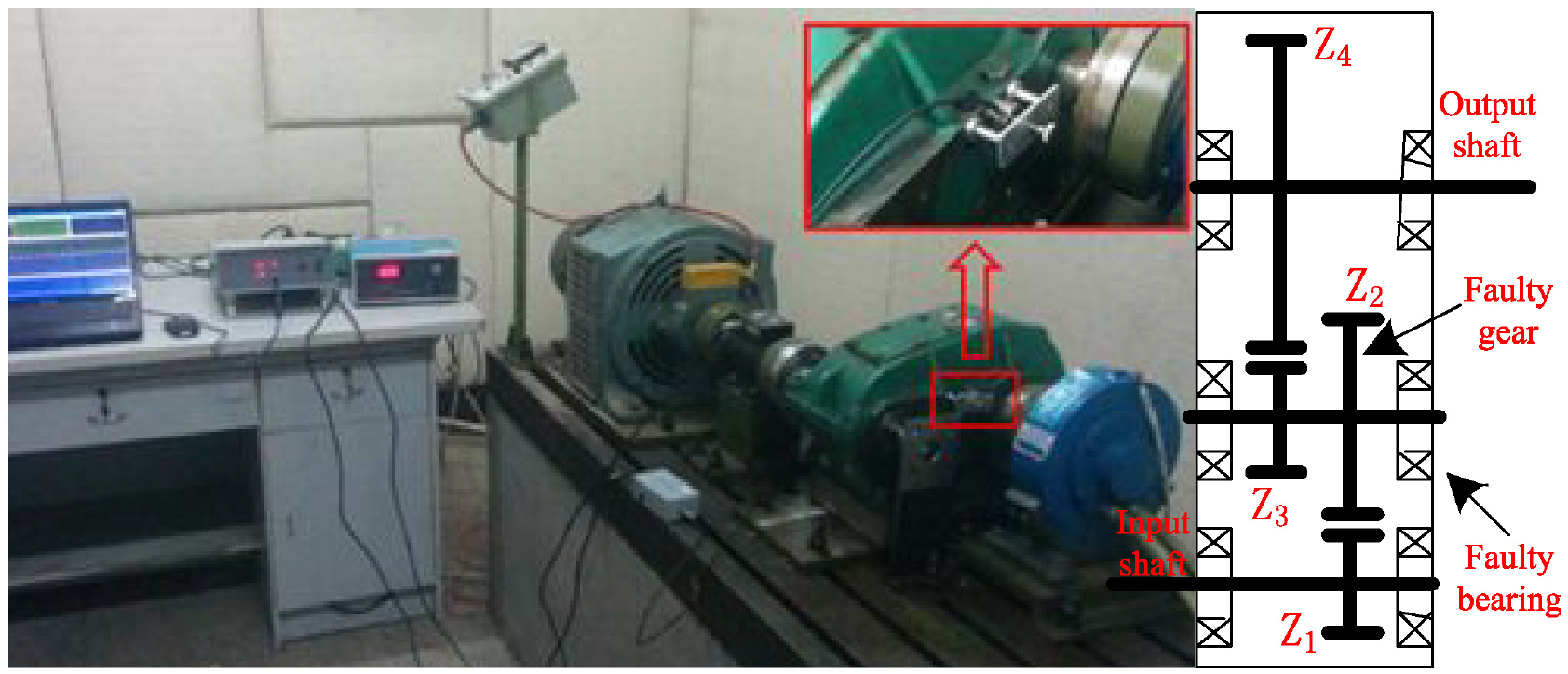
The experimental signal data is obtained from a gearbox fault test bench, using a second machine reducer as shown in Figure 14, the number of teeth is Z1 = 25, Z2 = 50, Z3 = 19, Z4 = 81, and the transmission ratio is 8.53. The fault bearing is a 6206 deep groove ball bearing, the fault type is a wire cut crack fault, crack width and depth are 1 mm. The acoustic emission sensor is SR150M single-ended resonant sensor whose frequency response range is 60−400 kHz. The system sampling AD resolution is 16 bits, and the sampling frequency is 1 MHz.
As shown in Figure 14 below, the gearbox test bench and test equipment used in the experiment are mainly composed of a motor, secondary reducer, speed and torque sensor, magnetic powder brake, acoustic emission signal sensor, preamplifier, acoustic emission signal collector, and computer.
During the operation of the gearbox test bench, the input shaft of the gearbox is driven by the motor to drive the overall operation of the gearbox. The output shaft of the gear box is connected to the magnetic powder brake, and the braking torque can be generated by the brake to replace the load when the load is required.
In this paper, the acoustic emission signal data under normal working conditions, bearing inner ring fault, bearing outer ring fault, and broken tooth fault are collected respectively under the non-load condition of the motor speed of 1492 rpm.
Specific implementation mode
The specific experimental steps are basically the same as in section 3.12. Firstly, the acoustic emission signal is decomposed by EMD, and then the IMF component with the largest kurtosis value is selected as the noise reduction signal, and the upper envelope is demodulated to obtain the upper envelope as the subsequent signal to be processed, and then the GASF transformation is performed on the envelope signal to construct the criterion matrix of each fault category, and finally calculate the matrix distance between the feature matrix of the new signal and the criterion matrix of each category. The fault classification is identified by the size of the distance distribution.
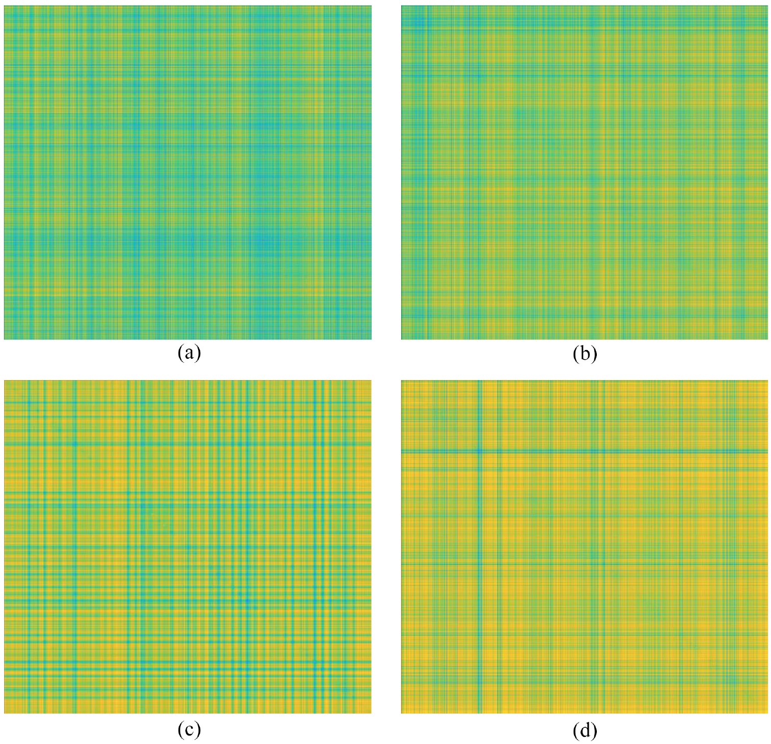
For acoustic emission signals with very high sampling frequency, to ensure the adequacy of fault signals, the sample data length is selected to be 1,000,000. Since the sample data is too long, PAA processing is required for the data before GASF data conversion. Finally, it is verified that the sliding window size is 10, which has the best comprehensive effect. Finally, a feature matrix size of 1000 × 1000 is obtained. Then the corresponding criterion matrices under different states are obtained, and their GASF images are shown in Figure 15.
In order to further validate the method, 70 groups of test data are extracted from each state of four different acoustic emission signals without exceeding the amount of test data, and fault diagnosis is carried out according to the method proposed in this paper. Finally, the overall classification accuracy of 280 sets of test data is 95.71%, indicating that this method can also get good results in the fault diagnosis of gearbox acoustic emission signals.
Influence parameter analysis
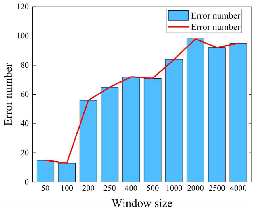
If the sample data is too long, to reduce the amount of data computation, the signal can be processed by sliding down sampling, but the change of the sliding window size will also affect the accuracy of the diagnosis. As the sliding window size increases. The change in the number of test samples is shown in Figure 16 below.
It can be seen from Figure 16 that with the increase of the sliding window, the number of errors of the test sample shows an increasing trend in fluctuations, and the accuracy of the method decreases with the increase of the window.
Compare with other methods
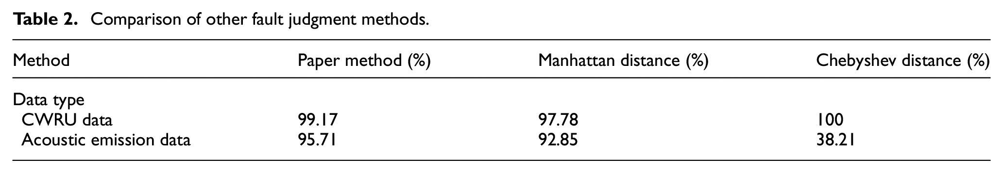
When using the criterion matrix to calculate the reference number comparison size and determine the fault category, in addition to using Euclidean distance, there are other methods for comparison, such as Manhattan distance and Chebyshev distance. The specific steps are similar to the above, after replacing the distance calculation of the method in the paper with the Manhattan distance and Chebyshev distance, the accuracy of the test sample is calculated and the accuracy of the method in the paper is compared, and the results are shown in the following Table 2.
Comparison of other fault judgment methods.
Conclusion
Aiming at the problem of fault signal diagnosis and classification of rolling bearing and gear of gearbox, this paper proposes a fault diagnosis method based on matrix distance feature on the basis of sliding window compressible GAF transformation. After filtering the fault signal with the EMD kurtosis value, the envelope signal is obtained by envelope demodulation, and then the one-dimensional fault signal is converted into a two-dimensional characteristic matrix by the GAF transformation method. Through the two-dimensional characteristic matrix of known fault category data, the criterion matrix of each category is constructed by using the method of matrix mean value. And fault diagnosis is carried out by measuring the distance between the two-dimensional features of the newly sampled data and the matrix of the criterion matrix, achieving fault classification.
Finally, the method proposed in this paper is validated using publicly available bearing fault data from the Case Western Reserve University and acoustic emission fault data collected from a gearbox test bench. The accuracy of fault classification is 99.17% and 95.71%, respectively. The results indicate that the method has good fault diagnosis effect and strong adaptability, and can achieve good diagnostic results on the vibration signal and acoustic emission signal of the gearbox.
Compared with other feature extraction methods for fault diagnosis, the feature extraction method in this method is simpler and accurate. It is not only suitable for vibration signals of gearboxes, but also for acoustic emission signals of gearboxes.
Footnotes
Declaration of conflicting interests
The author(s) declared no potential conflicts of interest with respect to the research, authorship, and/or publication of this article.
Funding
The author(s) disclosed receipt of the following financial support for the research, authorship, and/or publication of this article: The research is supported by Tianjin Technical Expert Project of China (Grant No.: 22YDTPJC00480) and Cooperative Scientific Research Program of Chunhui Projects of Ministry Education of China (Grant No.: HZKY20220603).