
Abstract
We propose a control structure for a quadrotor carrying a slung load with swing-angle constraints. This quadrotor is supposed to pass through the waypoints at specified speeds. First, a cascaded PID autopilot is designed, which adaptively gives attention to position and speed requirements as a function of their errors. Its parameters are found from an optimization problem solved using the PSO algorithm. Second, this controller’s performance is improved by adding the Complementary Controller employing an ANN. 5. Training data for the ANN is created by solving optimal control problems. The ANN is activated when the swing angle constraint is about to be violated. It is trained using optimal control values corresponding to the cases where the swing angle falls in a particular band about the upper swing angle constraint. Simulations are performed in a MATLAB environment. Finally, some of the simulation results are validated on a physical system.
Keywords
Introduction
In recent years, with the technological developments in unmanned aerial vehicles (UAV), studies on package delivery, 1 agricultural applications, 2 search and rescue in dangerous areas,3,4 and information gathering from desired regions,5–7 and military applications have gained momentum. 8 Load transportation is vital in all these applications. 8 Two different methods are being studied for carrying loads with rotary-wing UAVs. One can carry a load using a manipulator9–12 integrated into the vehicle. The other is to connect the load to the vehicle with a cable or rope.13–15 In vehicles with a manipulator, the vehicle’s inertia grows due to components associated with the manipulator – consequently, energy utilization of the vehicle with the manipulator increases. One of the biggest problems for UAVs is the short mission time. In addition, especially when it is required to perform agile movements, the growth in inertia will oppose the maneuvering. For these reasons, hanging loads seem more advantageous. However, using the suspended load method is also challenging because system dynamics change during the lift, hover, and flight. Even though we have not covered it in this study, we would like to emphasize that one of the important issues about load-bearing quadrotors is precise landing. This topic is covered in depth in Xuan-Mung et al. 16 and Xuan Mung et al. 17
As Khamseh et al. 4 highlighted, a complete mathematical model covering all phases of flight is the biggest challenge. Models are created assuming the cable or rope is constantly tense during flight. Flight profiles that violate these assumptions should be prevented during flight (e.g. the vehicle descends quickly). Usually, there are swings during the flight due to the quadrotor’s acceleration. These motions have distorting effects on the quadrotor’s dynamics.
A controller should be designed to make the vehicle follow the desired path and minimize these swinging effects. The controller designed in this study is carried out based on these considerations.
In the literature, extensive studies have been published to model the suspended load-bearing rotary-wing UAV systems. Modeling was carried out using the Udwadia-Kalaba Equations in Goodarzi et al. 18 and Almeida and Raffo, 19 the Euler-Lagrange approach in Lee et al. 20 and Lee et al., 21 the Newton-Euler method in Jain, 22 and the Kane method in Klausen et al. 23 In Pizetta et al., 24 the system dynamics are defined as the second-order Euler-Lagrange model while ignoring the aerodynamic effects. In Barikbin and Fakharian, 25 the Euler-Lagrange method was used, but the load’s motion was assumed to be planar rather than 3-dimensional. In this study, the controller is designed using the mathematical model detailed in Lee 26 based on the Euler-Lagrange approach.
Measuring and estimating suspended load oscillations is critical for controlling the system. The oscillation frequency caused by the suspended load has been investigated by Geronel et al., 27 in which the dynamic model is constructed by obtaining dimensionless equations of motion. A method is proposed to determine the vibration frequency of the payload during flight. In recent years, studies have been focused on the controller design for such systems to reduce the oscillations of the suspended load. In Sadr et al., 28 a nonlinear control algorithm is developed that applies a pulse to the system to prevent oscillation, whose amplitude and time locations are calculated by estimating the system’s natural frequency and damping ratio. Due to the quadrotor’s movements, the slung load will start to swing while moving to the desired point. This swinging action affects the quadrotor’s traveling motion. 29 The suspended load can create unstable oscillations due to its disturbing dynamics and reduce the performance of the UAV. They may even cause crashes in some cases. 30 Therefore, it has been studied for a long time to solve the difficulties of UAVs in carrying suspended loads. Controller and path planning is the most critical parts of these studies. In Jain, 22 a controller is designed for a quadcopter carrying a point-mass load with a rigid cable. Predictive control is considered for carrying the payload from point to point with swing angle constraints along the desired trajectory.23,24 Guerrero et al. 31 present a passivity based-controller design to minimize the load swing. However, a simplified 2D model is used in this study. In Kusznir and Smoczek, 32 sliding mode control is used for horizontal positioning and payload vibration damping, while a linearizing feedback controller is used for altitude and attitude control. In Yu et al., 33 the backstepping procedure is applied to design a controller for the load to follow a pre-determined trajectory by defining a virtual thrust force. They find the actual forces using this virtual force. Another controller based on the backstepping method is proposed by Dai et al. 34 to reduce the swing angle of the load. There, the swing angle of the suspended payload is estimated using the harmonically extended state observer. In Shi et al., 35 an adaptive control scheme with unknown mass transportation is proposed. Lee et al. 36 proposes an adaptive sliding mode controller to achieve the goal of altitude tracking control in the presence of considerable system parameter variations and the ground effect.
After choosing the controller type, its parameters should be determined to optimize the performance. Usually, evolutionary algorithms are preferred for this purpose; PSO (The PSO technique is used to design the PID controller to stabilize the humanoid robot,37,38) Ant Colony Optimization (ACO) technique, 39 Genetic Algorithm (GA), 40 Differential Evolution (DE), 41 (the pitch angle controller of a rocket system is optimized algorithm). Comparisons made by El-Ghandour and Elbeltagi 42 have demonstrated through in-depth studies that PSO is more efficient and has lower computational complexity simultaneously.
There are many reasons why Artificial Neural Networks are used in control applications. First, the self-learning ability of neural networks eliminates the use of complex and challenging mathematical analysis that predominates in many adaptive and optimal control methods. Second, it provides a nonlinear mapping capability to solve highly nonlinear control problems by incorporating the Activation Function into hidden neurons. Third, unmodelled dynamics and perturbations in the system are expected to be dealt with using an ANN. Thus, neural controllers can be applied over a broader range of uncertainty.
As ANN has proven to have excellent approximation and learning capabilities, they have become popular tools in control applications of nonlinear systems.43,44 A unified framework for describing and controlling nonlinear dynamical systems is proposed in Polycarpou. 45 The adaptive nonlinear control and the parametric method of adaptive linear control theory can be applied to perform stability analysis. Typical stable neural network approach control schemes based on Lyapunov training designs are given in Mughees and Mohsin. 39 Training neural networks using a backpropagation algorithm (BP) has dramatically increased the development of these structures in control applications. 46 Many research studies have proven the approximation capabilities of neural networks. 47 In this context, many neural control approaches have been developed with BP neural networks.45,48,49 Moreover, the ANN structure has been used in different control applications; Guo et al. 50 provides a decentralized robust optimal monitoring control scheme for the class of nonlinear systems interconnected with disturbances and actuator attacks, for which the optimal control problem is solved by NN-based adaptive dynamic programing.
We aim to make a quadrotor carry a suspended load following a given path without the load swinging too much. Here, the slung-load system is supposed to follow a path using the generalized waypoint guidance algorithm (waypoints and desired speeds are specified). The original contributions of this study are described below:
An autopilot is designed consisting of cascaded PID controllers for inner and outer loops. This autopilot is supposed to control the position and velocity of the quadrotor and prevent high swing angles of the suspended load.
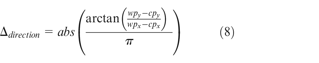
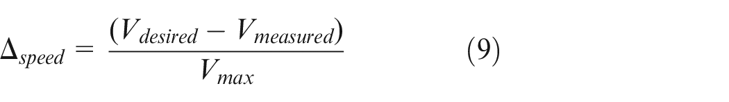
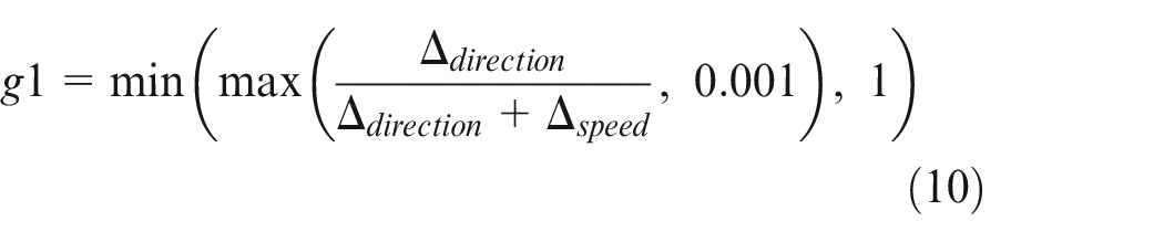
The primary controller adaptively changes (the percentage of) its attention to speed or position depending on its errors. While the PID coefficients are found, the controller gains associated with positions and velocities are adaptively tuned by gain adjustment (see equations (8)–(11)).
Finally, the whole structure is fine-tuned using delta force and torques produced by a Complementary Controller with an ANN to attenuate the oscillations if there is too much swinging.
Training data for the ANN is created by solving optimal control problems to calculate the attenuating delta force and torque inputs to the plant when the swing angle is above a certain threshold. These calculations are performed while the vehicle tries to follow specially chosen paths.
To the best of our knowledge, there is no such study for a slung-load quadrotor system.
The rest of the paper is organized as follows; Firstly, the dynamic model of the system is given in Section II. Secondly, the structure and design procedure of the controller are described in Section III. Section IV contains the experimental results. Then, this study is concluded in Section V.
Dynamic model
This section will describe the 3D dynamic model for the slung-load quadrotor system. It starts with the coordinate system definitions in the mathematical model, as shown in Figure 1. The mathematical model used in this study is borrowed from Lee. 26 The detailed derivation of this model can be found there.
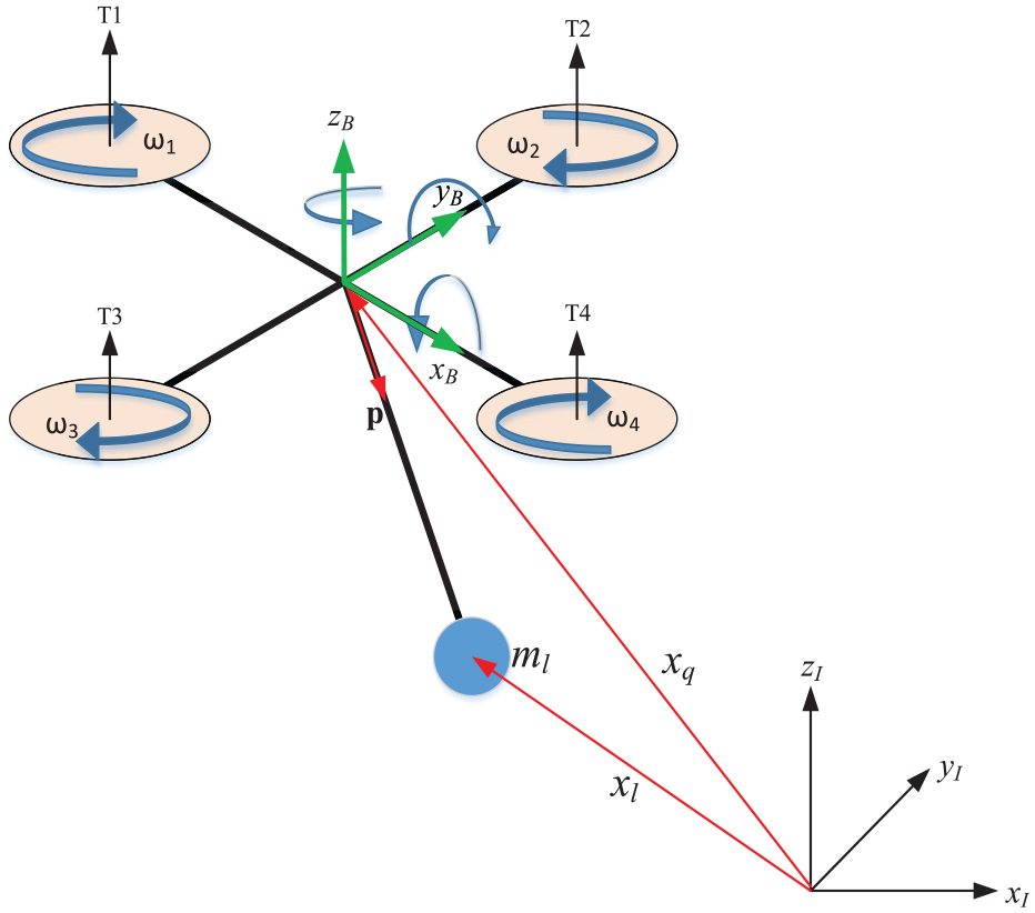
Slung-load quadrotor system coordinate frames.
This model is differentially flat; the flat outputs are the load’s position and the quadrotor’s yaw angle. Unlike Lee,
26
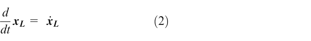
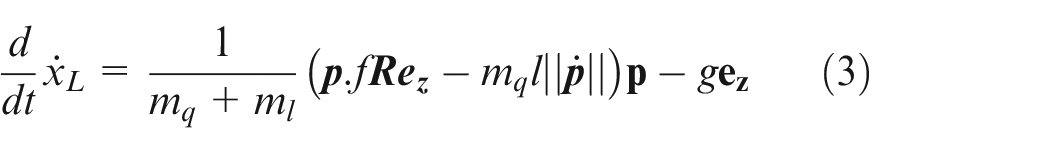
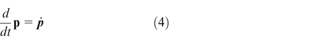
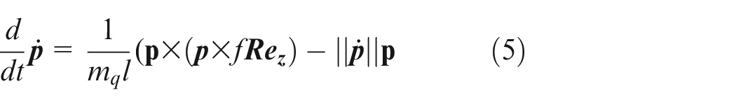
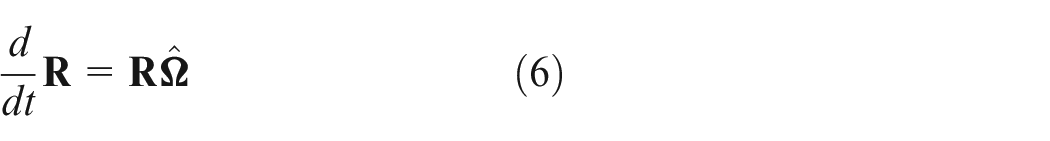
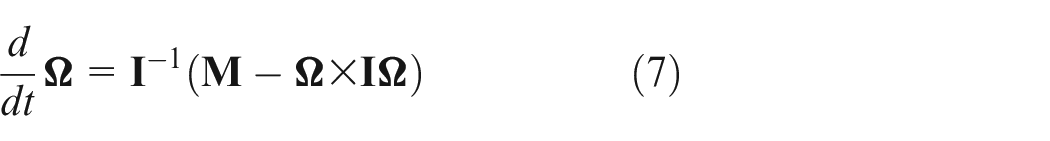
the 3D dynamic model is preferred over the flat model since we imposed constraints on the quadrotor’s position and attitude. Additionally, different from previous studies,46,51,52 we do trajectory planning for both the load and the quadrotor to avoid obstacles. The state vector is,
The dynamic model for the slung-load quadrotor system is valid under the following assumptions:
The payload is connected with a cable at the quadrotor’s center of gravity.
The cable is rigid, massless, and inelastic.
The quadrotor has no external disturbances or interactions, such as wind, except for the load.
The input vector
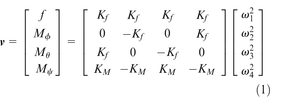
where
where
Controller design
Our study gives the waypoints the unmanned aerial vehicle should visit and the desired speed values at these points. When the system reaches a certain proximity to a desired waypoint, this point is considered already visited, and a command is produced to go to the next waypoint. Figure 2 shows this structure for two consecutive waypoints. In our study, as in the trajectory tracking approach, the entire path is not given, but only specific waypoints (the dashed lines between the waypoints are drawn to show the approach easily).
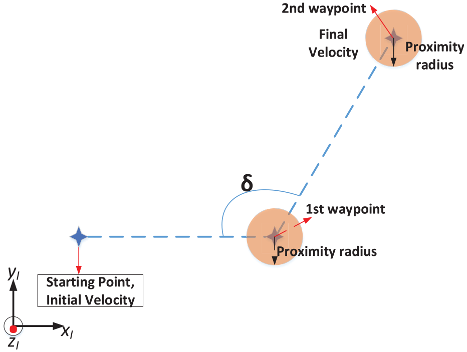
Waypoint geometry used in controller design.
The slung-load quadrotor system is an under-actuated system having 8 degrees of freedom (DOF) and 4 control surfaces. It is a challenging task to control this system with velocity constraints. The controller structure shown in Figure 3 has been created to overcome this challenge. In this figure, each controller block consists of a PID controller. The vehicle’s roll and pitch angles must be changed for position and speed control. Since we want to perform speed and position control, another block for gain adjustment has been added. The gain adjustment block adjusts effectiveness by changing the roll or pitch angles according to speed and position errors. This effect is achieved by calculating the

where
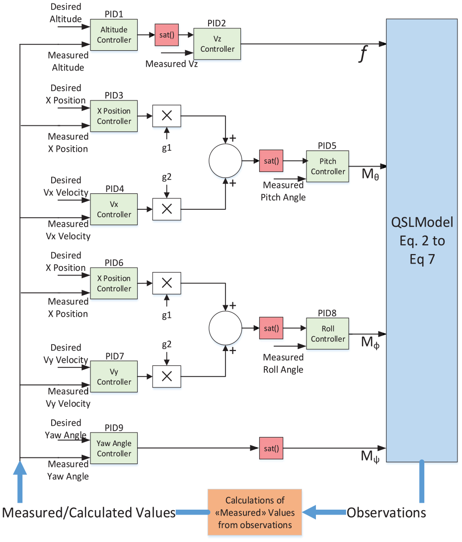
Controller structure without the complementary controller.
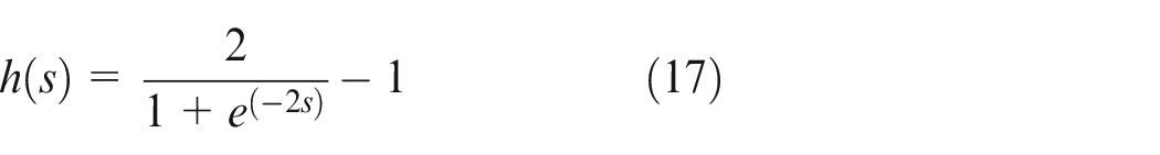
Tuning the PID coefficients has been proposed as an optimization problem solved using the PSO algorithm. The problem definition is given below in detail.
Definition of the optimization problem
The control objective is to ensure that all waypoints are visited in a certain order and at the desired speed at the waypoint in minimum time. The system must visit the waypoints sequentially. A proximity radius is defined for waypoints considered visited when the distance to a waypoint less than the proximity radius is. The proximity radius may change according to the task performed, which is considered one of the problem’s input parameters.
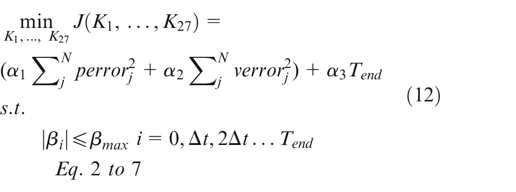
where
Details of the objective function calculation are given below.
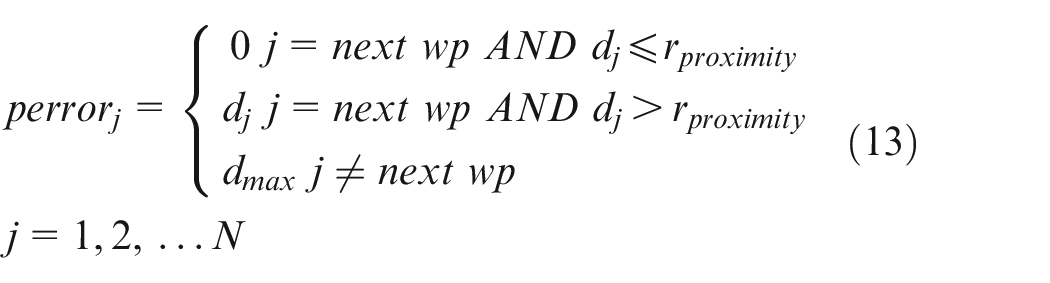
where,
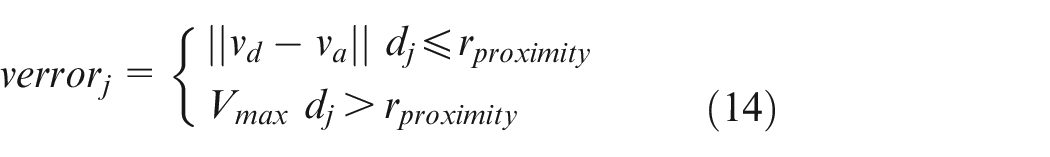
Since the speed objective is valid only within the radius of the proximity area, the function is written in parts, and the velocity error outside this region is considered the maximum allowable velocity value.
PID gains using particle swarm optimization
Our optimization problem (equations (12)–(14)) depends on the Simulink model; we prefer to use a derivative-free evolutionary algorithm. PSO is a population-based iterative algorithm.49,54 Populations are structured with some topology comprising bidirectional edges connecting particle pairs.
The power of PSO comes from the interaction of individuals and movement to a better objective value that occurs when the individuals interact. All particles in the same neighborhood communicate so they move toward their new position, influenced by the best objective value obtained by the individuals in the topology. Topologies of the neighborhood are scrutinized in Poli et al. 47
In PSO, many particles are positioned in the problem’s search space, each evaluating the objective function at its present location. Each particle in the swarm is composed of three vectors in
Data generation for ANN
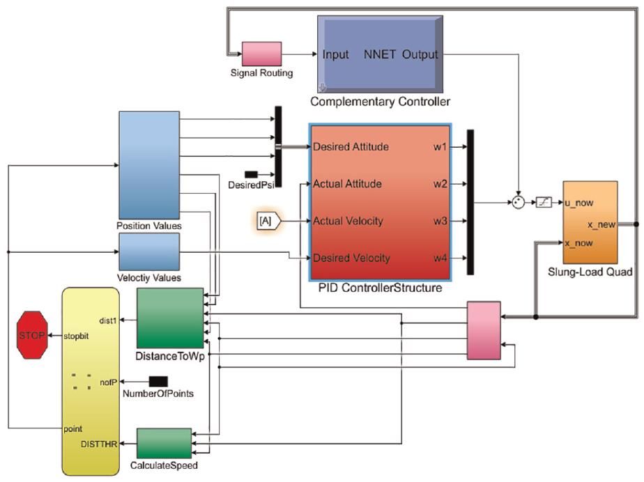
The controller structure given in Figure 3 was tested in many different scenarios. During these trials, if the vehicle is supposed to make a sharp turn between consecutive waypoints, the swing angle of the load may violate the constraints. This problem has been solved by adding a complementary controller, which computes the required controller inputs using an ANN. This structure (see Figure 4) with ANN creates complementary control inputs when necessary. It accepts velocity and position error vectors as inputs and generates necessary force and moments as its outputs. If the swing angle of the load is within the specified range, this structure will not contribute to the overall control inputs.
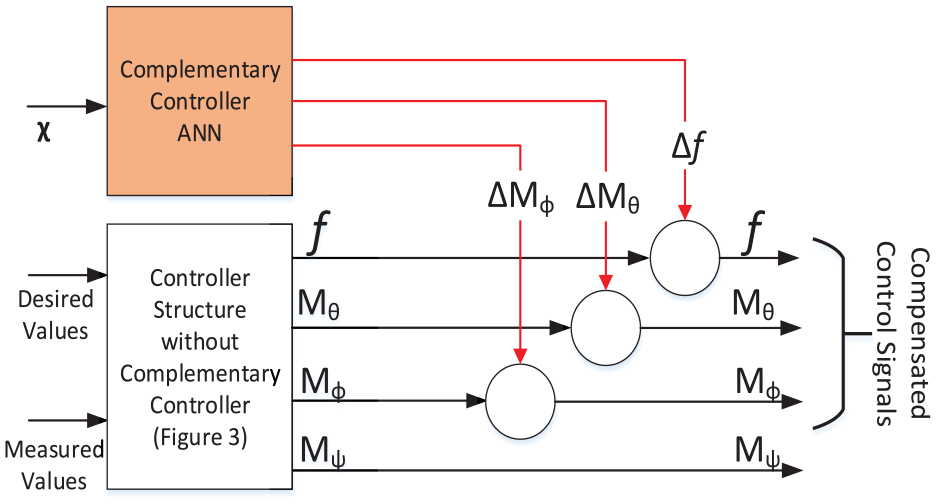
Overall controller structure with ANN.
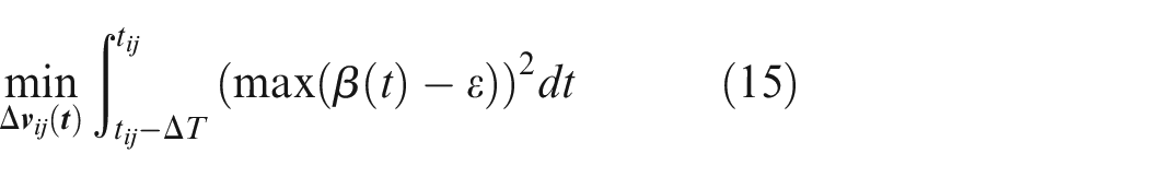
The input data for training the ANN has been created by running the structure shown in Figure 3 for different and challenging scenarios. Instances that did not meet the angle constraint were found in the results of these runs. Figure 5 shows the plot of a swing angle obtained from a scenario and the points that do not satisfy the constraint value. A particular optimal control problem is solved for each point (indicated by red dots in Figure 5) in the zoomed image. In these optimal control problems, the aim is to obtain the value of the complementary control inputs that will bring the swing angle below the constraint value. A complementary input
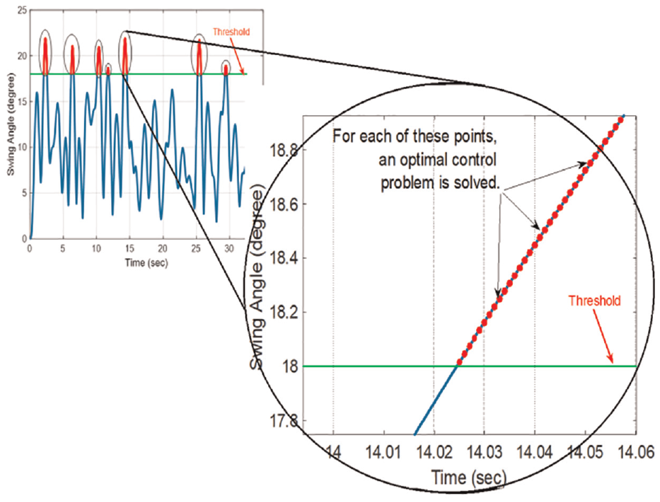
Points at which swing angle constraint is violated.
subject to
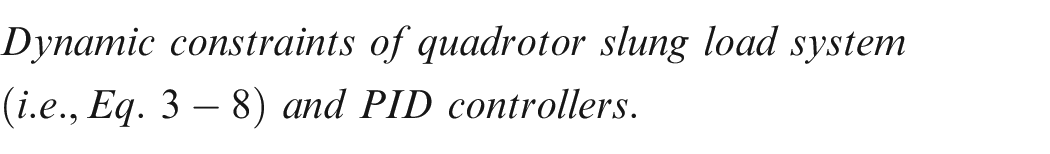
where
Input:
Output:
Training of the ANN
The scaled conjugate gradient backpropagation algorithm Møller 55 is used because it avoids the line search per learning iteration. Instead, this algorithm uses gradient calculations to update weights instead of the Jacobian calculations used by other methods such as Levenberg-Marquardt and Bayesian regularization. The feedforward calculation has been given as follows;
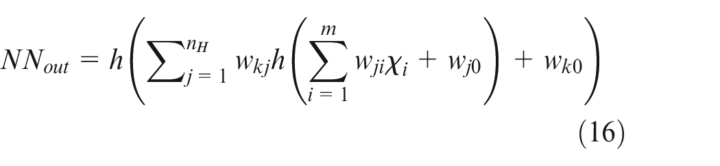
where the subscript
Simulation results
Results without using the complementary controller
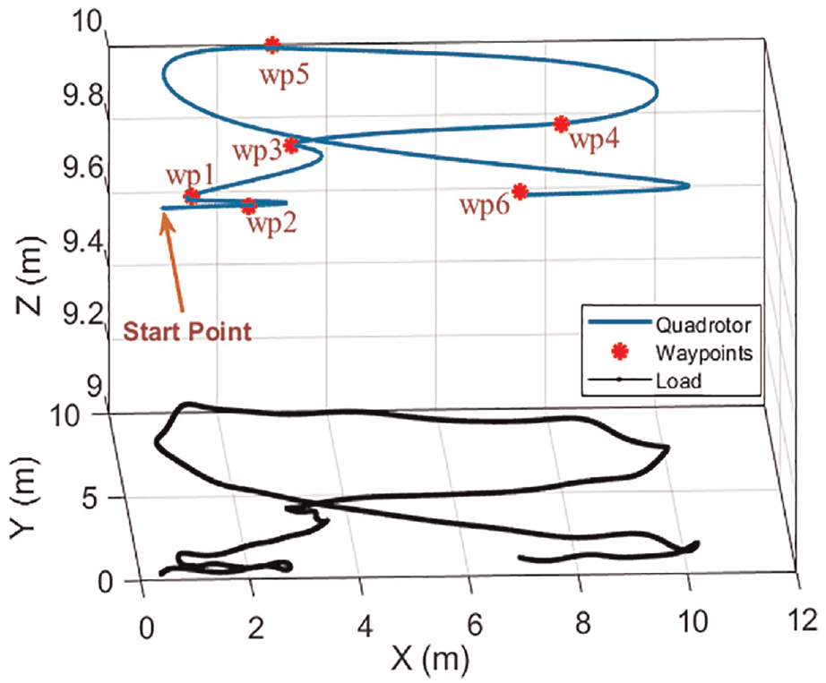
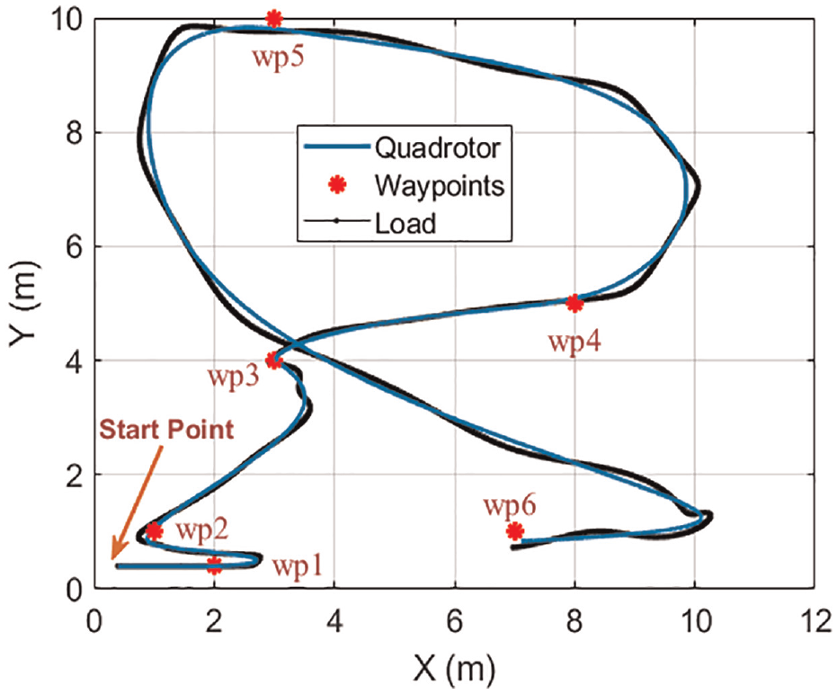
A sufficiently challenging scenario with a 30° swing angle constraint is suggested to determine the PID coefficients using Algorithm 1. The top view of the resultant paths for the quadrotor and slung load is given in Figure 6. As shown in Figure 7, where the swing angle of the load is plotted with respect to time, the maximum swing angle has been obtained as 9.83°. In Figure 8, the graph of the vehicle’s speed is presented, and the speeds at the waypoints are marked. It is observed that the speeds at the waypoints are close to the desired speeds. There are minor deflections from desired speeds due to the swinging of the load. A more challenging scenario with very sharp turning points is used in this new study (Scenario-2). In this scenario, first, PID coefficients are found using an angle constraint of 15°.
PSO-based PID tuning
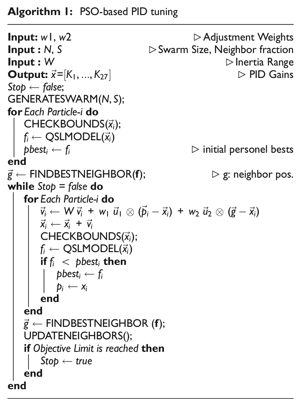
Top view of the path of quadrotor slung-load system (Scenario-1).
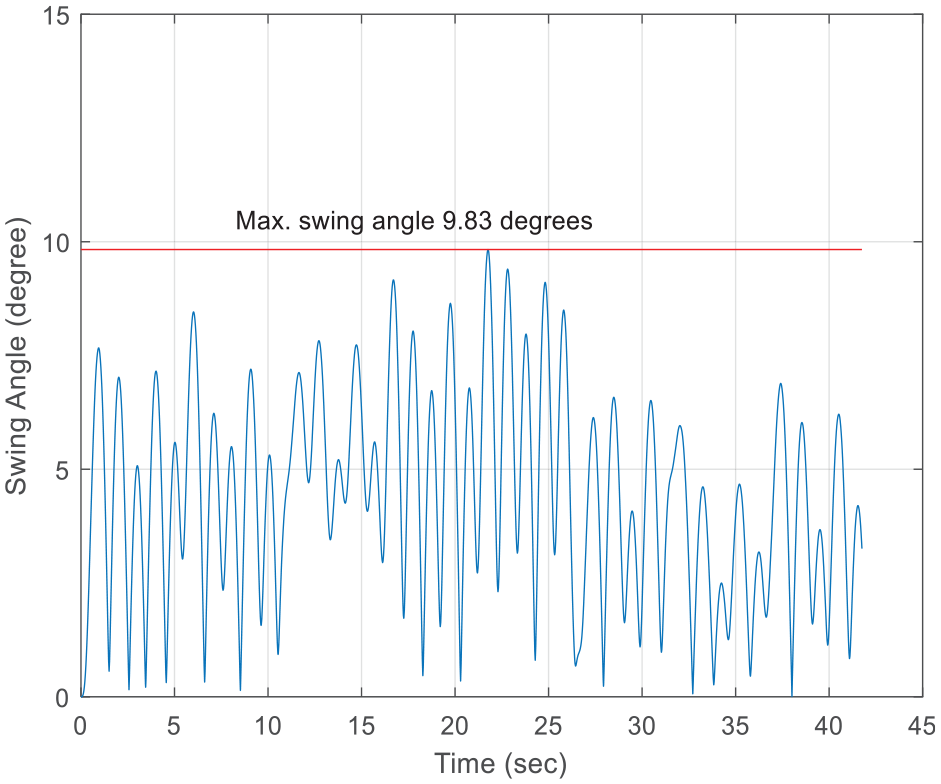
The swing angle of the load versus time (Scenario-1).
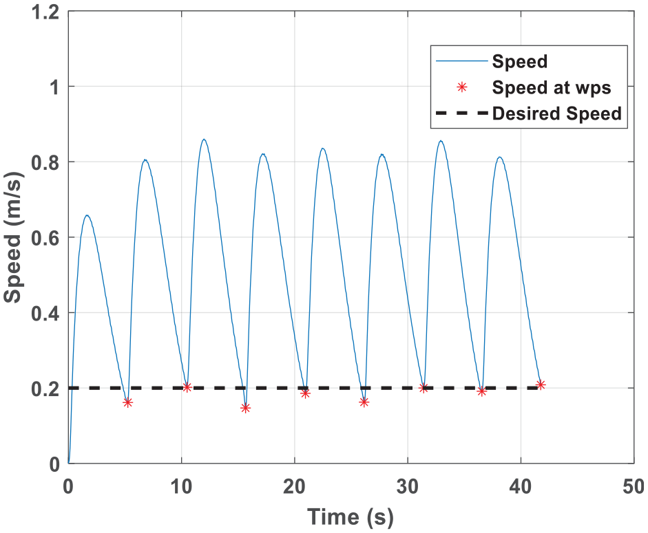
Quadrotor’s speed versus time (Scenario-1).
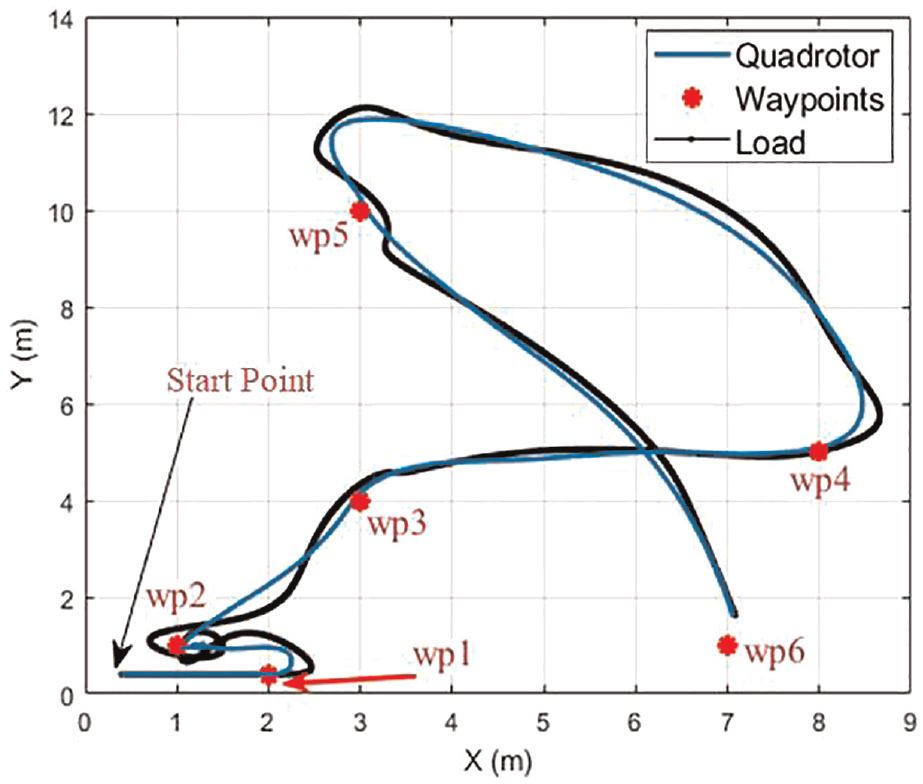
The resultant paths followed by the quadrotor and slung load are presented in 3D in Figure 9. The top view of these paths is shown in Figure 10. The swing angle of the load is presented in Figure 11. As observed in this figure, the maximum swing angle is 12.49°. In Figure 12, the vehicle’s speed with respect to time is given.
3D view of the path of quadrotor slung-load system (Scenario-2_1).
Top view of the path of quadrotor slung-load system (Scenario-2_1).
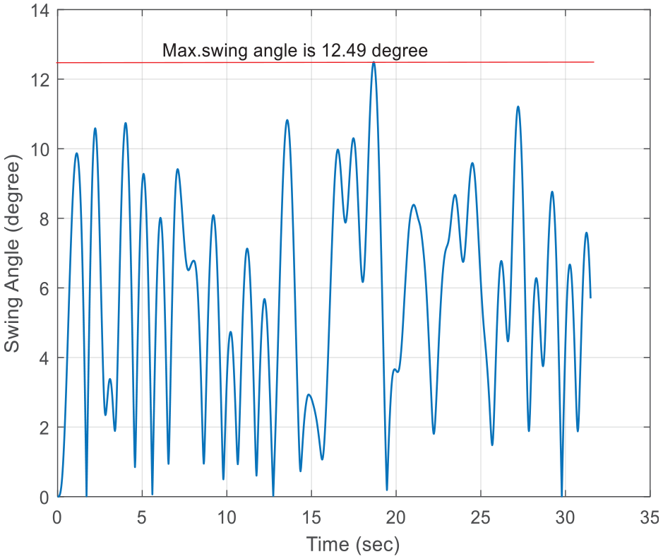
The swing angle of the load versus time (Scenario-2_1).
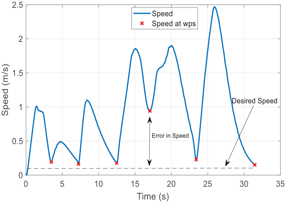
Quadrotor’s speed versus time (Scenario-2_1).
Afterward, we wondered what happens to PID coefficients and the system’s performance if the swing angle constraint is relaxed to 30° (using the same scenario with a different swing angle constraint, i.e. Scenario-2_2).
When we run Algorithm 1 with this constraint on this scenario, we obtain the paths given in Figure 13, and the corresponding swing angle is given in Figure 14. The maximum swing angle is 25.81° in this case. We want to point out that by relaxing the system’s swing angle constraint (i.e. Figures 11 and 14) from 15° to 30°, task duration is decreased from 35.619 s to 25.764 s. This (i.e. decrease in task duration) is an expected result because as the system is more relaxed, it can behave faster to minimize costs further.
Top view of the path of quadrotor slung-load system (Scenario-2_2).
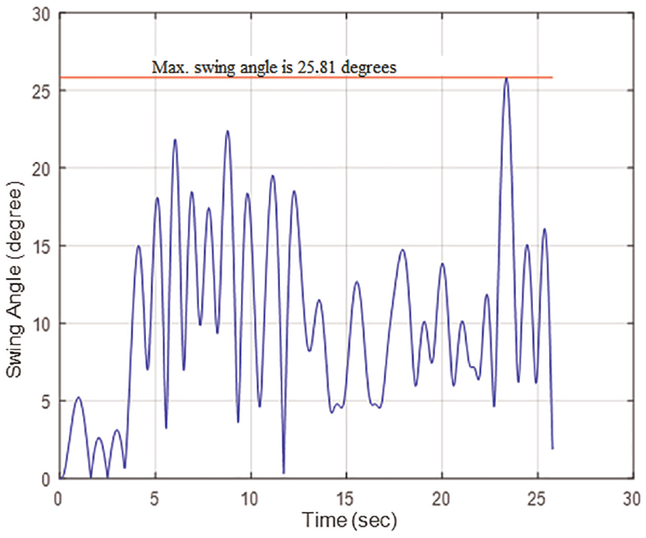
The swing angle of the load versus time (Scenario-2_2).
The PID coefficients found in the scenario with 15° swing angle constraint are tested on a new scenario (Scenario-3) shown in Figure 15. The resultant maximum swing angle (14.78°) can be observed in Figure 16, which is not much different than the result in Figure 11.
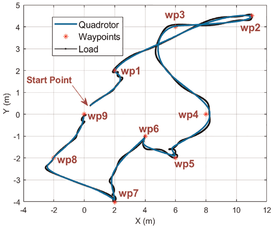
Top view of the path of quadrotor slung-load system (Scenario-3).
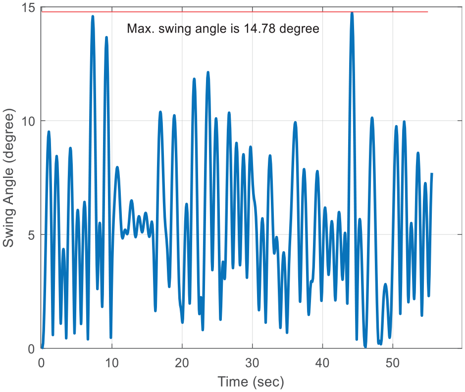
The swing angle of the load versus time (Scenario-3).
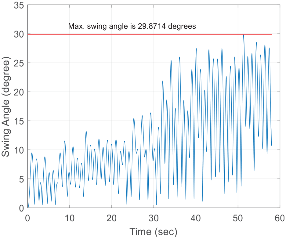
To check the sensitivity of PID autopilot coefficients concerning the path in the chosen scenario and the constraints, we performed the final test on a new scenario (Scenario-4), shown in Figure 17. This scenario has many sharp turns that may cause swing-angle constraint violations. Indeed, when the controller structure in Figure 3 is used, the swing angle of the load is given in Figure 18. The swing angle constraint for this scenario is 30°, but the resultant swing angle is about 38°. Therefore, since optimizing the PID coefficients for every possible path, desired speeds, and swing angle constraint is impossible, we have concluded that the autopilot structure should be extended/complemented in Figure 4.
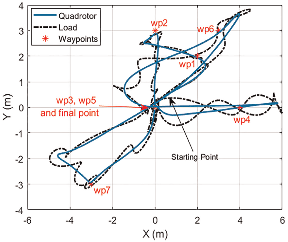
Resultant paths using controller structure without the complementary controller (Scenario-4).
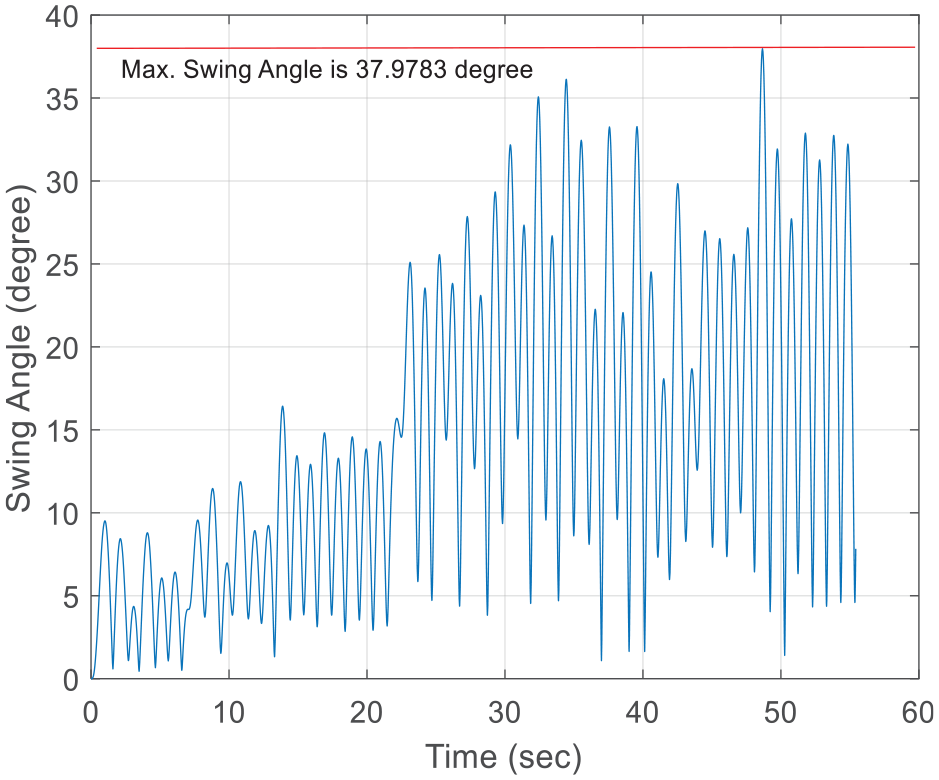
Swing Angles using controller structure without the complementary controller (Scenario-4).
Results using the complementary controller
The training data for ANN in improved structure is obtained from Figure 18 when the swing angle constraint was 30°. This new structure (with ANN) is tested on the same scenario (Scenario-4) with a swing angle constraint of 20°.
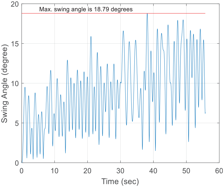
The results are shown in Figure 19; the path with the same set of waypoints is given. In this case, the control structure given in Figure 4 is employed. The ANN part is activated automatically when the swing angle of the load is within 18°–22°. Otherwise, it does not generate any delta inputs. As shown in Figure 20, the constraint is violated around 40th seconds by 0.0077°.
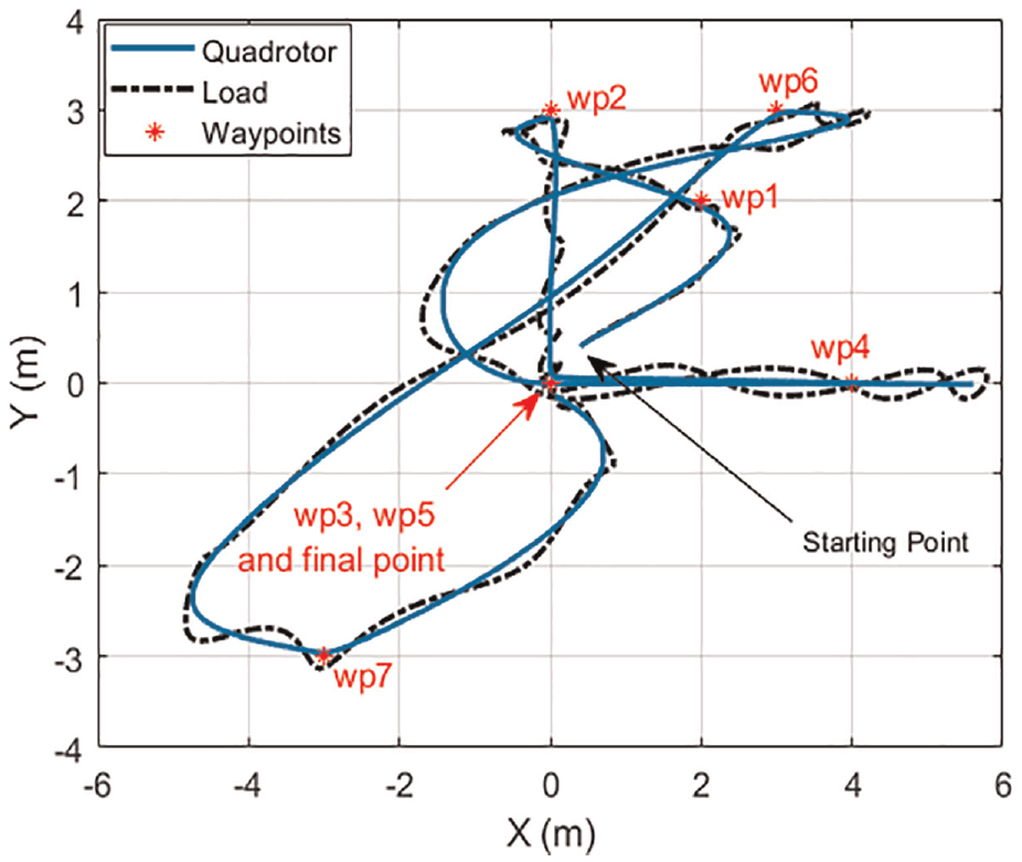
Resultant paths using controller structure with complementary controller (Scenario-4).
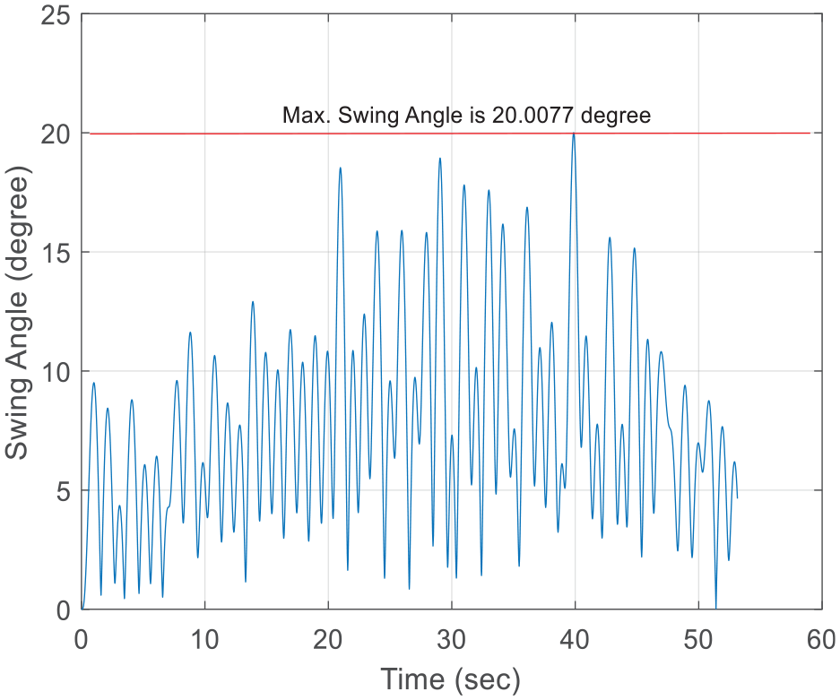
Swing Angles using controller structure with using the complementary controller (ANN has been trained for
Figures 21 to 23 give delta inputs for thrust, roll, and pitch moments. As can be seen from these figures, the ANN structure is activated when the swing angle is within the defined interval (i.e. between 18° and 22°). Also, delta inputs are saturated, as in the case of PSO. We now change the swing angle constraint from 20° to 17° to better observe the Complementary Controller’s performance. Data is collected from the band
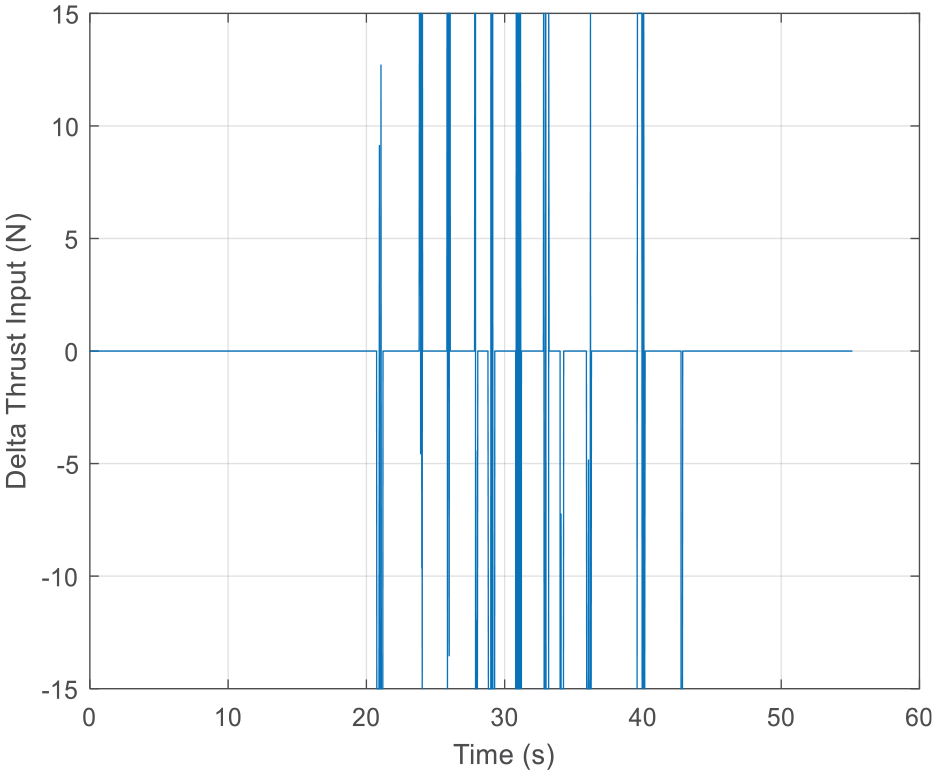
Thrust generated by complementary controller versus time (Scenario-4_1).
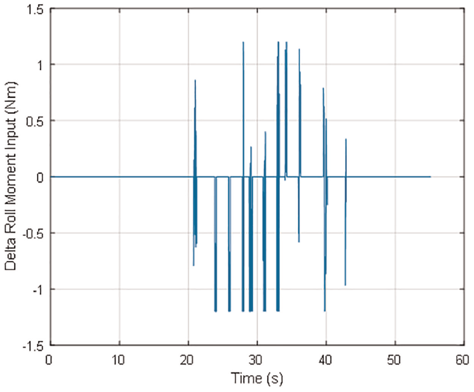
Roll Moment. It was generated by complementary controller versus time (Scenario-4_1).
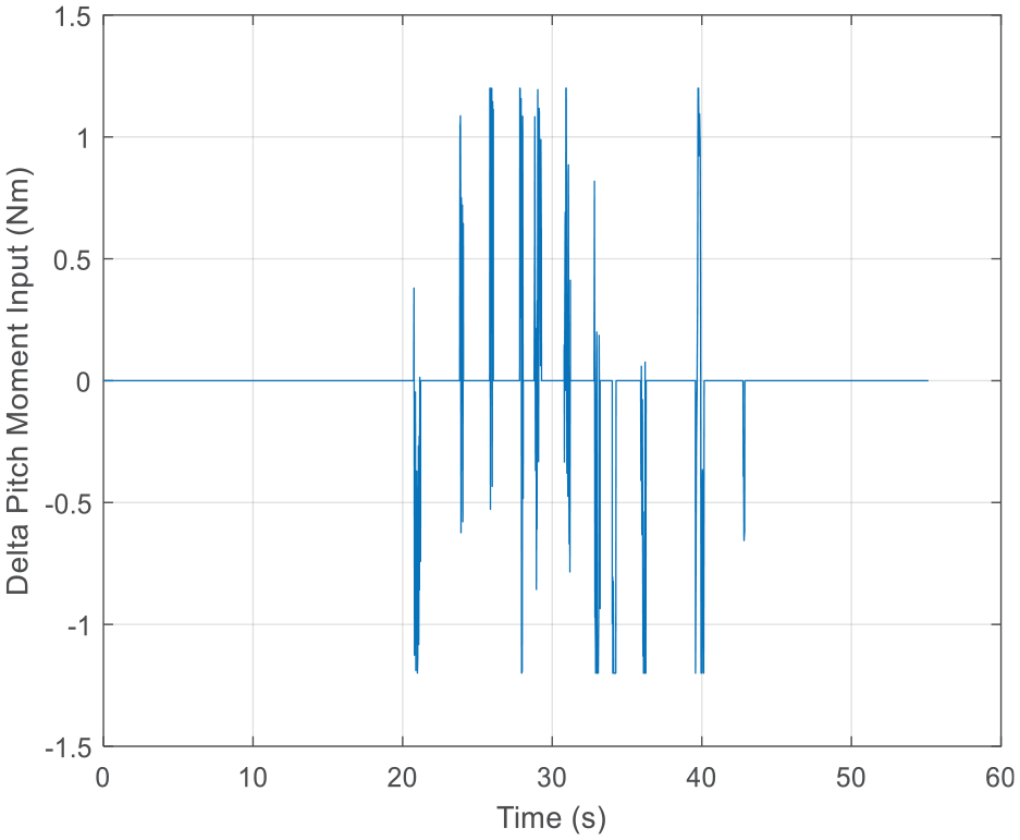
Pitch Moment. It was generated by complementary controller versus time (Scenario-4_1).
Swing Angles using controller structure with using the complementary controller (ANN has been trained for
Swing Angles using controller structure with using the complementary controller (ANN has been trained for
The overall simulation structure, including the state flow diagram (yellow block), is given in Figure 26. In this model, the state flow diagram manages waypoint guidance.
Overall Simulation structure constructed in MATLAB/Simulink.
A few of these simulation studies were realized physically in an experimental setup. We use a similar method in Li et.al. 56 to measure swing angles. Firstly, swing angle measurements of slung load were tested in a laboratory medium using the setup in Figure 27. The measurement accuracy was verified using a Single Board Computer (SBC) and a camera at the top of the setup. Next, the angular displacements of the slung load measurements were obtained using the same (Inertial Measurement Unit) IMU in the quadrotor-slung load system. Later, this swing angle measurement setup is integrated into a quadrotor.
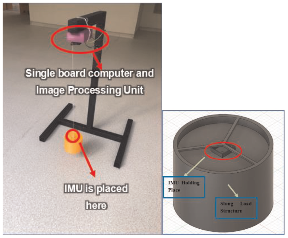
The swing angle measurement setup to collect IMU data.
Conclusions
This study designed a controller for a quadrotor carrying a suspended load. The quadrotor is supposed to reach its destination by passing through waypoints with speed constraints. This problem is solved successfully using the proposed complex control structure in Figure 4. In this structure, the primary controller adaptively changes the gains for speed and position as a function of their errors. The Complementary Controller is activated whenever the swing angle constraint is violated. The resultant structure performs much better than the one without the complementary structure. Simulations have been performed in MATLAB/Simulink environment. Measurements of the swing angle are first obtained in a laboratory setup, then tested on a quadrotor in the open field.
Studies on this problem will be extended to the slung load case with multiple quadrotors.
Footnotes
Appendix
Notation
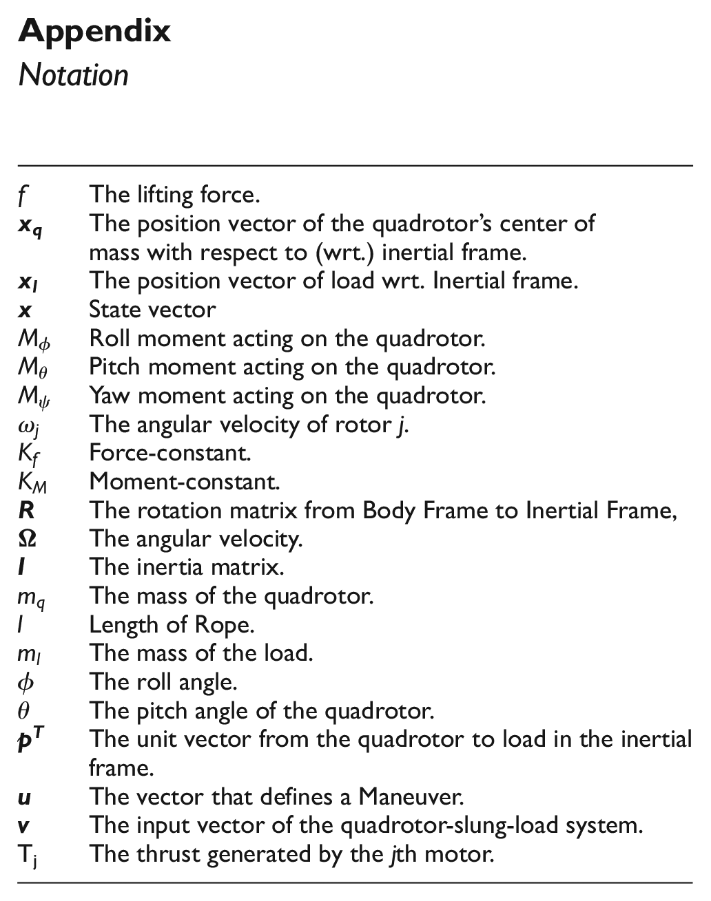
| The lifting force. | |
| The position vector of the quadrotor’s center of mass with respect to (wrt.) inertial frame. | |
| The position vector of load wrt. Inertial frame. | |
| State vector | |
| Roll moment acting on the quadrotor. | |
| Pitch moment acting on the quadrotor. | |
| Yaw moment acting on the quadrotor. | |
| The angular velocity of rotor j. | |
| Force-constant. | |
| Moment-constant. | |
| The rotation matrix from Body Frame to Inertial Frame, | |
| The angular velocity. | |
| The inertia matrix. | |
| The mass of the quadrotor. | |
| l | Length of Rope. |
| The mass of the load. | |
| The roll angle. | |
| The pitch angle of the quadrotor. | |
| The unit vector from the quadrotor to load in the inertial frame. | |
| The vector that defines a Maneuver. | |
| The input vector of the quadrotor-slung-load system. | |
| Tj | The thrust generated by the jth motor. |
Declaration of conflicting interests
The author(s) declared no potential conflicts of interest with respect to the research, authorship, and/or publication of this article.
Funding
The author(s) received no financial support for the research, authorship, and/or publication of this article.