
Abstract
This paper proposes a control strategy to achieve minimum wake-induced power losses in a wind farm. At first, the axial-induction-based wake model is developed to consider the aerodynamic wake interactions among wind turbines. To optimize the generated power of the whole wind farm, the axial induction factor of each wind turbine is calculated by the genetic algorithm. As a supervisory controller, each wind turbine’s optimal axial induction factor calculated by the genetic algorithm is implemented as a setpoint of each wind turbine’s internal controller. In the internal control loop, a comprehensive controller is designed to track the commanded axial induction factor. In the partial load region, the commanded axial induction factor was attained by tuning the generator torque. In the transient and full load regions, the blade pitch angle is tuned to keep the generator speed and torque at the rated values. The performance of the proposed control strategy is investigated through case studies, including three different wind speeds and a time-varying wind speed case in a 3 × 3 wind-farm layout. The simulation results show the satisfactory performance of the proposed approach.
Introduction
Renewable energies have numerous socio-economic benefits, including lower carbon emissions, lower air pollution, a growing number of jobs, and improved reliability in conjunction with rapidly falling technology costs. One of the fastest-growing renewable energy technologies is wind power. The installed capacity of wind power increased by a factor of 75 in the past two decades and doubled between 2014 and 2020. As the technology matured, control strategies have been developed for wind turbines to attain maximum energy at the lowest cost. Generally, wind power system control has three important purposes: minimize the structural loads to extend turbines’ lifetimes, maximize power, and maintain grid integrity. 1
Menezes et al. 2 presented a review of different wind turbine control strategies. Depending on the wind speeds, various inputs, including the blade’s pitch angle and generator torque, are employed to control the wind turbine. The fraction of power in the wind extracted by the turbine is a function of the tip-speed ratio. The tip-speed ratio of a wind turbine is the ratio between the tangential speeds of the blade’s tip and the wind speed. The generator torque control and blade pitch control should be implemented to adjust the rotor speed at different wind speeds and consequently tune the rotor axial induction factor and power performance. 3 Figure 1 shows the power curve of an NREL 5 MW wind turbine, 4 which is typically the same in modern wind turbines. In general, four regions could be recognized in the power curve. In region 1, there is no power production. To maximize power output in region 2, the generator torque is controlled while the pitch angle is held constant at its optimized set point. In region 3, while the generator torque is held fixed at its rated value, the pitch angle of the blades is controlled to reduce extra loads on the blades. In this region, the rotor speed and the power have been regulated to their rated values by a pitch controller. In region 4, due to high wind speeds and hence high loads on the blades, the wind turbine will stop power production. 5
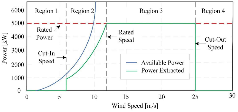
Operating regions of NREL 5 MW wind turbine. 6
Large amounts of existing literature on the topic of wind turbines are related to the control of wind turbines and wind farms (see, e.g. refs.7–13). Wind turbines are installed in a configuration known as a “wind farm,” which functions and is linked to the power grid as a single electricity power plant. A large wind farm’s annual total power loss usually ranges from 10% to 20% due to the aerodynamic effects of upwind turbines on downwind turbines. 14 After some distance downstream of the turbine, the wind flow recovers its original speed, and additional turbines can be installed. This distance varies with the wind speed, the turbine’s operating conditions, the ground’s roughness, and the atmosphere’s thermal stability. A common rule of thumb specifies five rotor diameters in cross-wind directions and ten rotor diameters in the main direction as the minimum spacing between the individual turbines. 15 Furthermore, the turbines’ operating conditions should be controlled to optimize the wind farm’s power production.
In the development of wind farm control algorithms, it is essential to have an appropriate wake model. 16 Several analytical models have been developed for wake modeling (e.g. refs.17–26). Also, there exist some computational wake models (see, e.g. refs.27–29). Moreover, the development of wake models has continued to achieve more quick and accurate models. A simple wake model that considers wake meanderings for implementation in the wind farm layout optimization problems was represented by Hu. 30 Recently, Ti et al. 31 developed a high-efficiency wake model based on machine learning and computational fluid dynamics. However, analytical wake models are extensively used in wind farm control.
In conventional wind farms, each wind turbine tracks its own maximum power point (Maximum Power Point Tracking, MPPT). This strategy does not result in maximum power extraction from the whole wind farm because the generated wakes from upstream wind turbines significantly decrease the power outputs of the downstream ones. Therefore, some researchers have focused on cooperative control of the whole wind farm to maximize the total output power. 32 Redirecting the wakes of the upstream turbines to be away from downstream turbine faces is investigated in Fleming et al. 33 and Howland et al. 34 In some research, the wind turbine’s axial induction factor is utilized to control the wake effects. The axial-induction factor, a, is the fractional decrease in wind velocity between the free stream and the turbine rotor. 35 In axial induction-based wind farm control, the axial induction factor of the turbines is tuned by controlling the blades’ tip speed ratio and pitch angle to recover the flow.
Annoni et al. 32 discusses the contrasts between the axial induction-based model of the wind farm and the high-fidelity model, such as SOWFA. Also, certain modifications to the model based on axial induction are presented to improve the results. Bartl and Sætran and Saetran 36 conducted an experimental investigation of the axial induction factors of two wind turbines, and the overall array efficiency of the two turbine configurations is mapped based on the tip speed ratio and the pitch angle of the upstream turbines. Scholbrock 37 modified the axial induction factors of a column array of wind turbines using optimization techniques in order to boost the wind farm’s overall output. Siniscalchi-Minna et al. 38 developed an axial-induction-based control algorithm to distribute the power of each wind turbine in order to maximize the power reserve.
In contrast to conventional methods of wind farm control, where each turbine is controlled independently, this article controls all wind turbines in a coordinated and integrated manner. The architecture of the wind farm control system includes a supervisory control for the entire wind farm that employs a genetic algorithm to optimize the wind farm power by calculating the axial induction factors and internal controls for each wind turbine that regulate the supervisory level commanded axial induction factors. In this regard, an axial-induction-based analytical model simulates the wind turbines’ wakes and their interactions in the wind farm. A wind farm power curve is also developed to demonstrate the superiority of the proposed control architecture in increasing the output power, similar to a single wind turbine. In summary, this paper considers the following set of contributions: (1) optimizing the whole wind farm generated power; (2) considering the aerodynamic wake effects among wind turbines; (3) developing two-layer control architecture, including a supervisory level for the entire wind farm and internal controls for each wind turbines; (4) proposing the wind farm power curve to visualize the superiority of the developed method.
The other sections of this paper are organized as follows: The wind farm model and the wind turbine dynamics are presented in section II, the control strategy of the wind farm is introduced in Section III, and the simulation results and discussion are presented in section IV. Finally, the conclusion is depicted in section V.
Wind farm model
According to the actuator disk theory, wind turbine rotor power (
where
For a wind farm consisting N number of wind turbines, total produced power is

where
Wake model
An appropriate wake model should reasonably model the wake parameters in both cases of wake behind the wind turbine and interacting wakes in a wind farm. Axial-induction based wake model32,33 is utilized in this study. In the case of a single wind turbine, velocity deficit in downstream of the turbine is defined as, 41
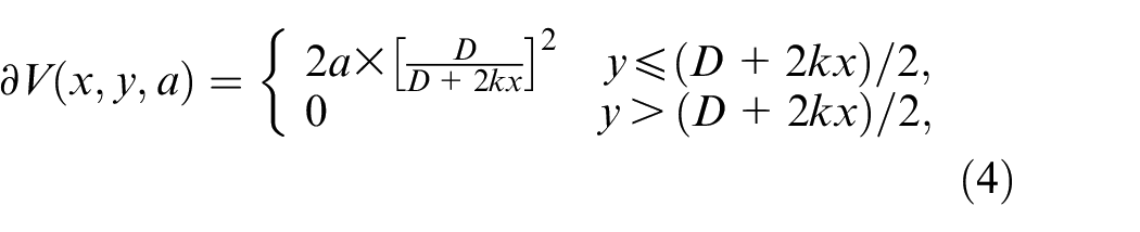
where

(x, y) coordinate system used in the definition of wake model for a single wind turbine.
In this study, It is assumed that yaw controller in each wind turbine would adjust x-axis with wind direction. In the case of wind farm, velocity deficit function should be capable to reveal both the effects of upstream turbines wake on the downstream turbines and the interacting wakes, as illustrated in Figure 3.
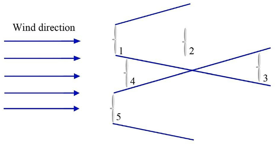
Schematic of interacting wakes in a wind farm with specific layout. 41
According to the axial-induction based model, the velocity deficit at rotor plane of each turbine in a wind farm is represented as, 35
where
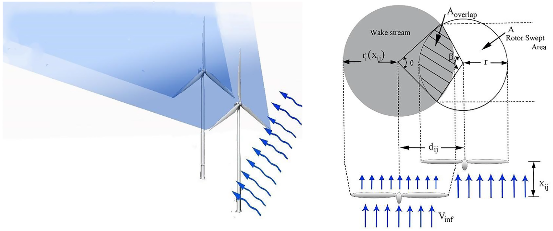
Schematic illustration of partial shadowing between upstream wind turbine wake and downstream turbine. 42
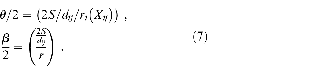
According to the Figure 4, the overlap area could be represented as follow,
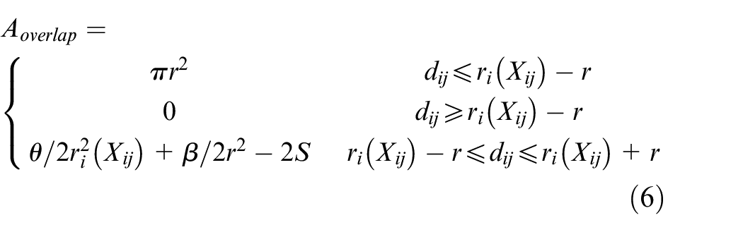
where,
Wind turbine dynamic
A reduced order dynamic model of wind turbine is utilized in this study as, 40
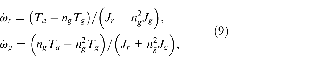
where

in which
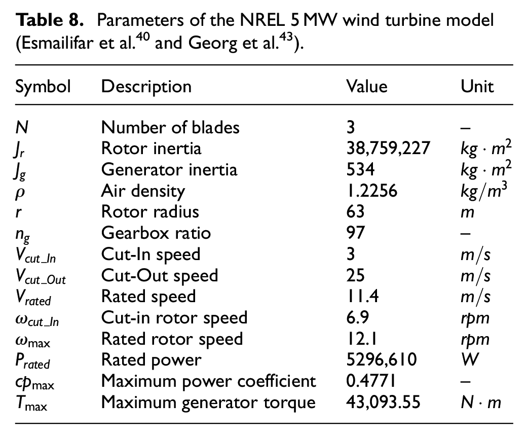
Parameters of the system
According to the actuator disk theory, aerodynamic power and thrust coefficients are represented as, 15
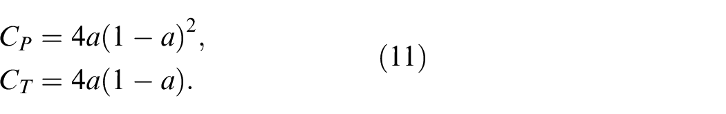
NREL 5 MW is a concept reference wind turbine which has been considered as a case study in several research works. In Annoni et al., 32 equations (11) are implemented in the simulation of an NREL 5 MW wind turbine with a correction factor equal to 0.8051.
Georg et al. 43 have approximated the aerodynamic rotor torque coefficient of NREL 5 MW as,
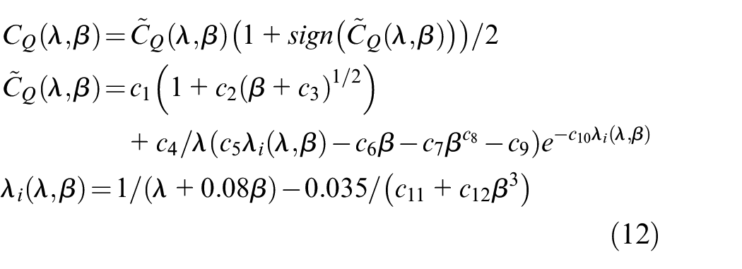
where the constant parameters
Constant coefficients of the
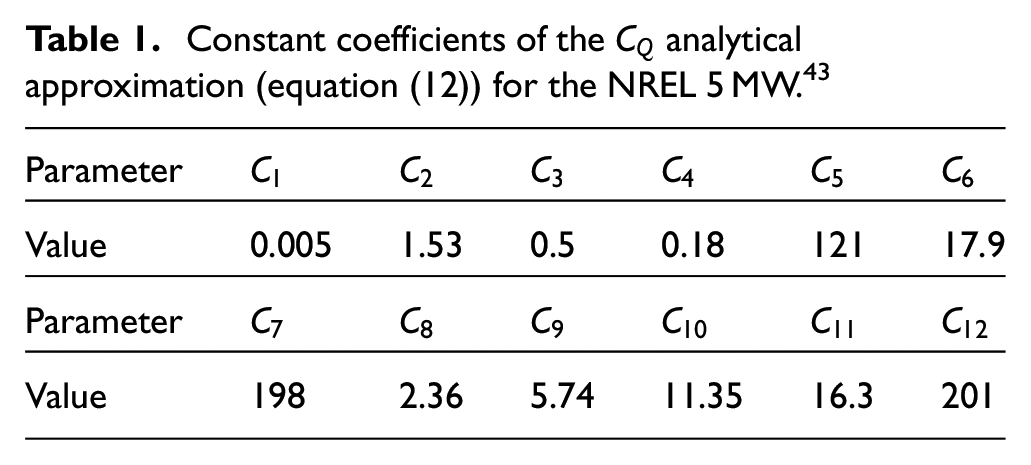
A similar approximation has been utilized for rotor thrust coefficient as,
where the constant parameters
Constant coefficients of
Control strategy
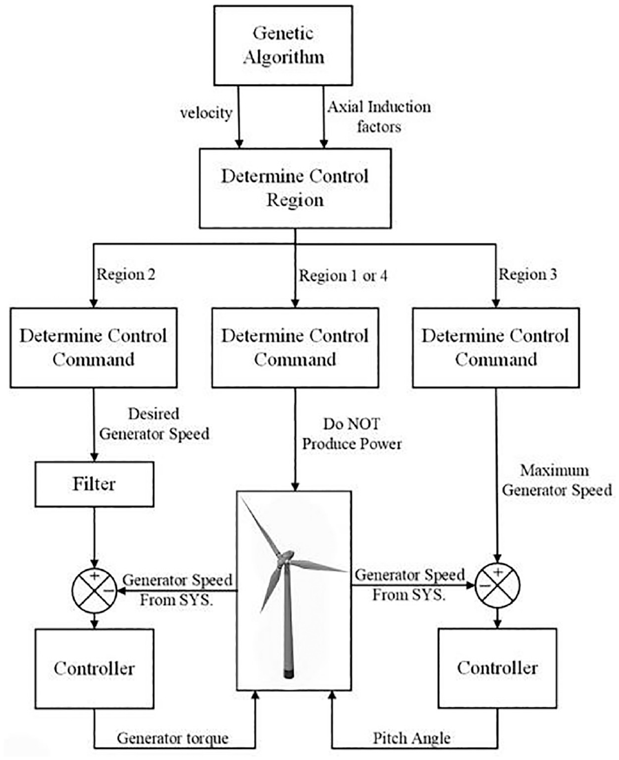
In conventional wind farm control, each wind turbine tracks its maximum power point, considering the local wind value. The present study will perform wind farm control in a centralized framework. In order to maximize the power output of the farm, the aerodynamic interactions between wind turbines will be reduced via the control of each wind turbine. Wind farm optimization will be performed utilizing the proposed axial-induction-based wake model. Each wind turbine’s optimized axial induction factor, determined from the wind farm supervisory level optimization process, is given to each internal controller. Consequently, wind turbine generator torque and blades’ pitch angle are controlled to meet the desired set points. The control mentioned above strategy of the wind farm is summarized in Figure 5.
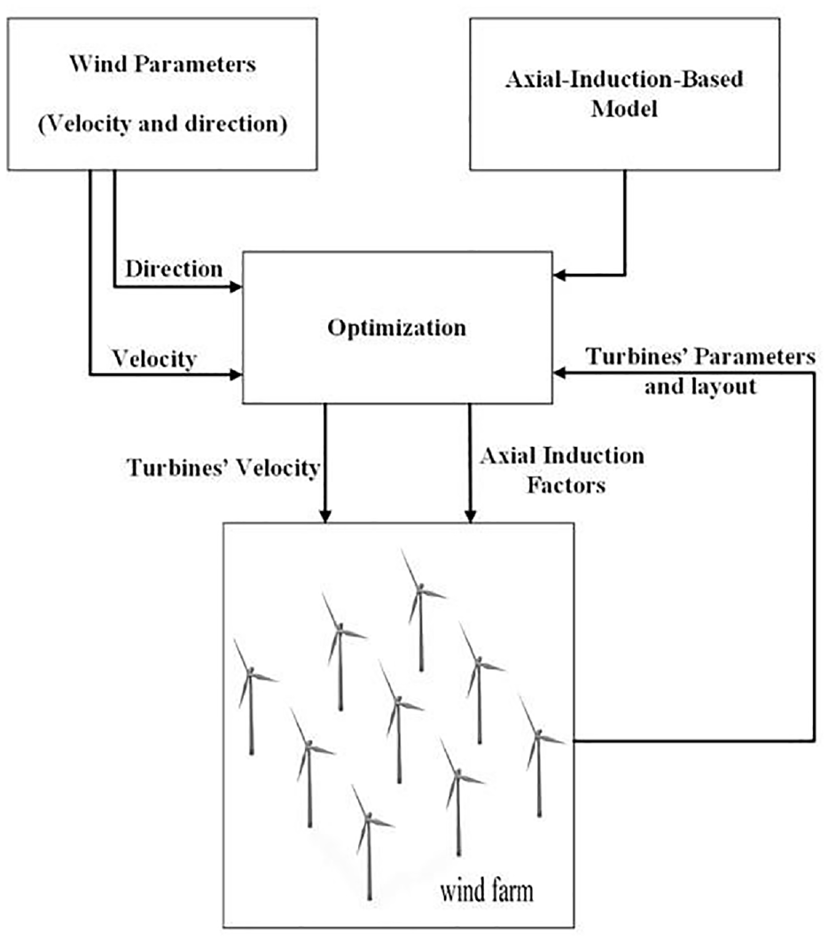
Flow chart of wind farm supervisory controller, external controller, working principle.
When wind turbines achieve their nominal power (i.e. working in region 3 of their power curve according to Figure 1), generator output power and angular speed should be kept constant to their nominal value. Hence, the supervisory controller could not change their operating set points. Therefore, the supervisory controller would optimize only those wind turbines operating in region 2 of their power curve.
Supervisory control
The supervisory control employs a genetic optimization algorithm to maximize the wind farm’s electrical power (equation (3)) by adjusting wind turbines’ axial induction factors. The optimization block in Figure 5 shows the relation of the genetic optimation algorithm with other control parts.
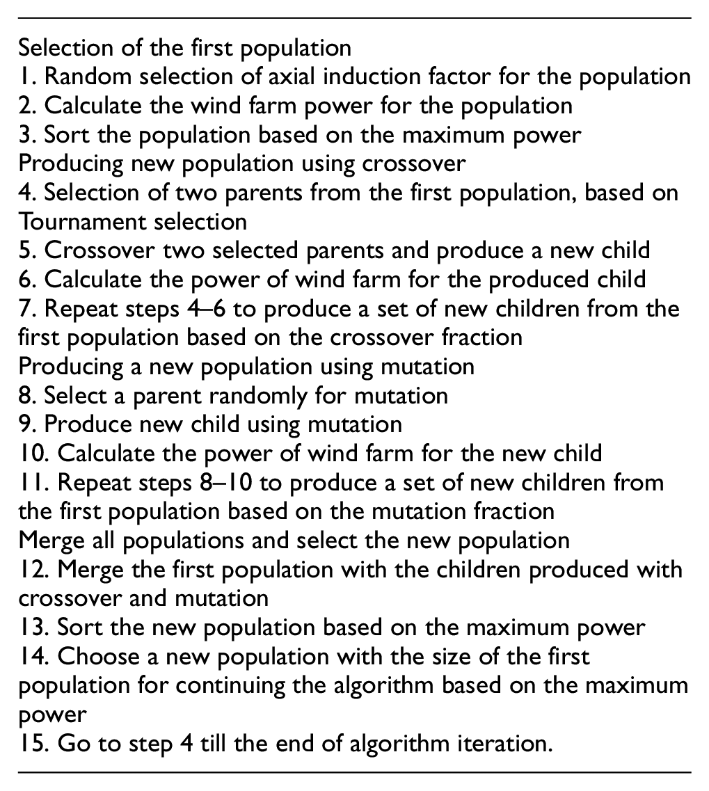
The genetic algorithm consists of four main steps. At first, a set of axial induction factors is selected randomly, and the wind farm power is calculated to make the first population. Then, a fraction of new children will be produced from the first population using the crossover. The selection of parents is based on their merit. It means that a set of parents with greater wind farm power is more likely to be selected for crossover. After that, the mutation is used on the first population to produce a fraction of new children from the first population. In the end, three populations have merged, and the new population with the same size as the first population is chosen based on their merit for continuing the algorithm. The algorithm is presented as follows:
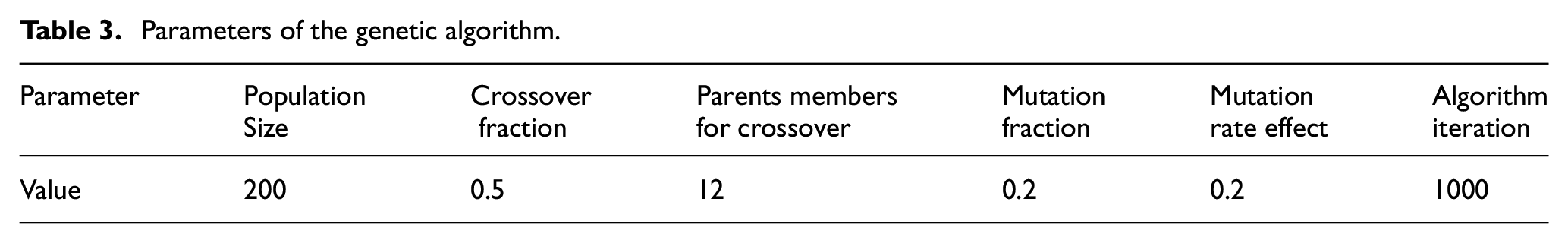
The parameters of the genetic algorithm that is set to supervisory level optimization are stated in Table 3.
Parameters of the genetic algorithm.
After wind farm power optimization, the optimized axial induction factor and wind velocity for each wind turbine are commanded to the internal controllers to adjust the operating conditions of each wind turbine individually.
Internal control
The function of the internal control loop is to control each wind turbine to achieve the desired set points determined by the supervisory controller. For turbines operating in region 2 or 3 of their power curves (as illustrated in Figure 1), the control input is generator torque (
For turbines operating in region 2 of their power curve, the controller tunes the generator’s torque and speed to achieve the required set point while the blade pitch angle is held fixed at the optimum value of
Flow chart of internal controller working principle.
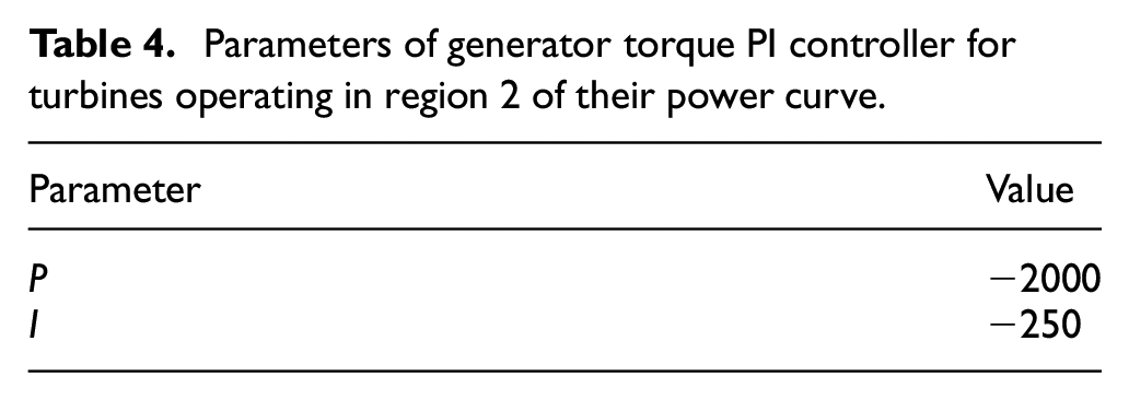
Finally, a filter is implemented to check the desired generator speed not exceed the rated value. It should be noted that the generator torque controller is a simple PI controller. The corresponding PI gains are tuned for NREL 5 MW, which are shown in Table 4.
Parameters of generator torque PI controller for turbines operating in region 2 of their power curve.
For turbines operating in the region 3 of their power curve, the generator torque and speed are held fixed at their rated values and the controller tune the blade pitch angle to achieve the desired set point via gain scheduled control methods. However, the aerodynamic behavior of wind turbines is highly nonlinear which should be considered in blade pitch control. 43
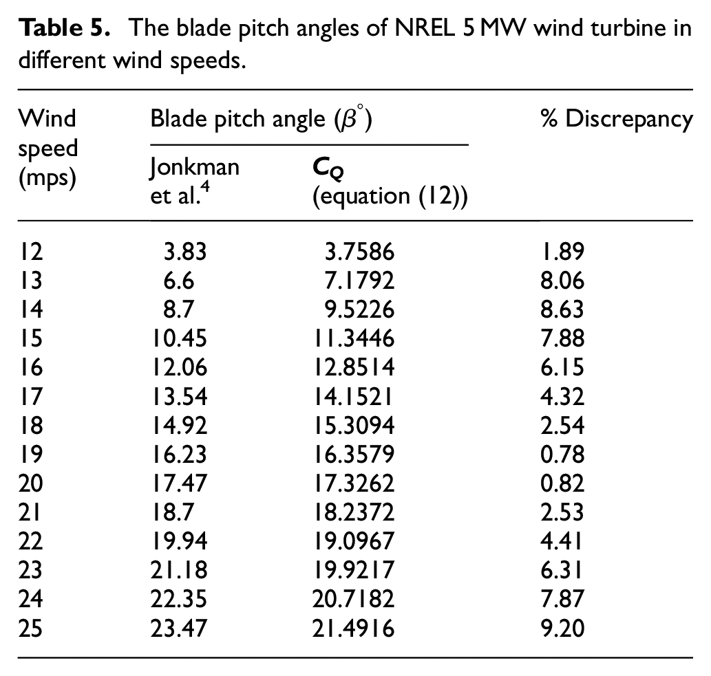
The appropriate blade pitch angle in different wind speeds is determined in design phase of wind turbines. Usually, these data are available for wind turbines. Also, solving equations 12 could lead to blade pitch angle versus wind speed. For NREL 5 MW wind turbine, the result of two aforementioned methods has a few discrepancies reported in Table 5. A little discrepancy, maximally 9.2%, is found between the pitch angles of NREL 5 MW turbine in region 3 that are reported in Jonkman et al. 4 and the result of the solving its aerodynamic rotor torque coefficient (equations (12)).
The blade pitch angles of NREL 5 MW wind turbine in different wind speeds.
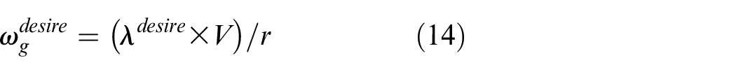
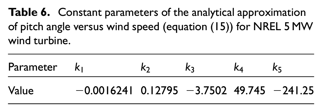
In this study, the available data of blades pitch angle versus wind speed will be implemented. An analytical expression could be interpolated to these data as,

where the constants (
Constant parameters of the analytical approximation of pitch angle versus wind speed (equation (15)) for NREL 5 MW wind turbine.
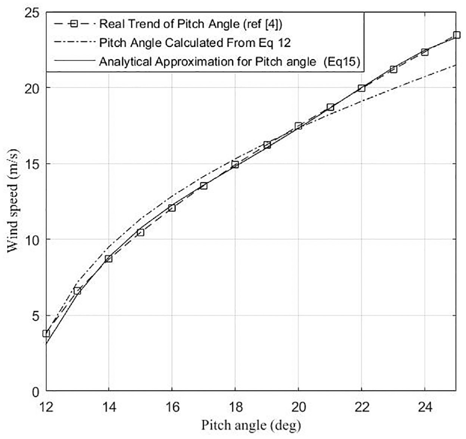
The Accuracy of analytical approximation of pitch angle of NREL 5 MW versus wind speed.
Between regions 2 and 3 of the power curve, there is a transition region where the generator speed reaches its maximum value. This region continues to the point where generator torque touches its maximum value. The control strategy in this transition region is similar to that of region 2, while the control function is to maintain generator speed instead of tracking the maximum power.
Using the aforementioned analytical relation in conjunction with a filtered derivative PID controller (equation (16)), the blade pitch angle will be controlled.
where, P, I, and D are the main parameter of the PID controller, and N is Filter Coefficient.
while the corresponding parameters are presented in Table 7.
Parameters of the implemented PID controller for blade pitch angle control.
Simulation results
Assumptions
A wind farm including nine NREL 5 MW wind turbine units with the same design parameters and are distributed in an array of the form of Figure 8 is considered in this section. The wind velocity and direction are assumed to be constant and predefined.
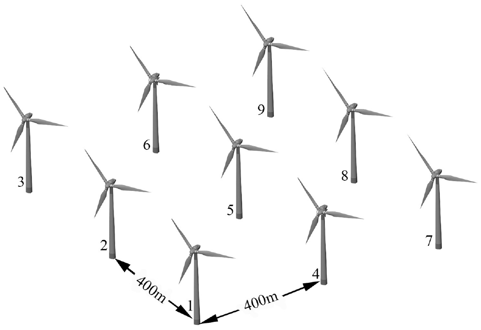
Wind farm layout, including 9 units of NREL 5 MW wind turbine in square array with equal cross-wind and downwind distances.
The description and all values of the NREL 5 MW parameters are tabulated in Table 8.
The simulation results are represented in the following sections. First, the wind farm’s overall performance will be studied through three cases of wind speeds. Obtained results depict the excellent performance of the proposed control strategy over the conventional ones. Afterward, the results concerning the performance of individual wind turbines at different wind speeds will be represented to highlight the local performance of the proposed control strategy at the wind turbine level.
Wind farm level
Three cases of wind velocity at the same blowing direction will be considered in the simulation of the supervisory level performance of the wind farm. In the first case, the velocity is set to 15 m per second, and for the second and third cases, wind velocities are assumed to be 12 and 9 m per second, respectively.
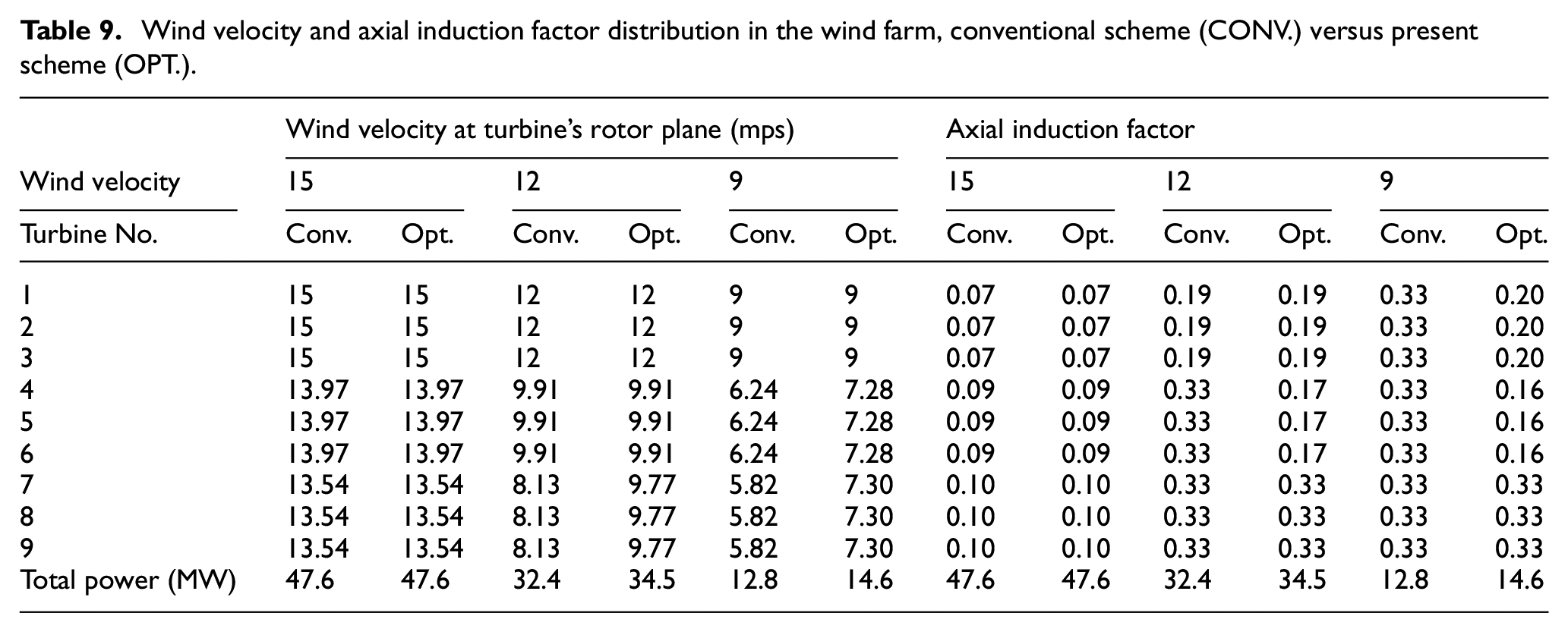
The simulation results (Table 9) reveal that:
For wind velocity of 15 m/s (case 1): all wind turbines are working in the full load region of their power curve (Region 3 of Figure 1). Therefore, the axial induction factors and velocity deficit of all wind turbines are determined based on their rated power. Hence, the supervisory level optimization has no influence on each wind turbines working conditions. In this case, wind turbines working conditions are determined by their internal controllers, individually.
For wind velocity of 12 m/s (case 2): the first row (turbine numbers of 1, 2, and 3) are working in the full load region of their power curve. Hence, their axial induction factors are calculated based on their rated power. Turbines locating in the second and third rows of the farm are working in the partial load region of their power curve. Hence, their optimum working conditions should be determined by the supervisory unit of the farm using genetic algorithm.
For wind velocity of 9 m/s (case 3): all wind turbines are working in the partial load region. Hence, the optimum values of the velocity deficit and axial induction factors should be evaluated by the optimization procedure in the supervisory level.
In cases 2 and 3: All turbines located in third row of the farm are working at their maximum power coefficients. These turbines should extract as much power as possible from wind flow because they have no aerodynamic effects on any other wind turbines.
As represented in the last row of Table 9, the utilized wind farm control scheme could improve the overall power production of the plant significantly.
Wind velocity and axial induction factor distribution in the wind farm, conventional scheme (CONV.) versus present scheme (OPT.).
Wind farm power curve, as a demonstrative concept is developed in this study (see Figure 9). Similar to wind turbine power curve concept, wind farm power curve is a graph that indicates how large the electrical power production of the farm will be versus wind speeds. Consequently, some important parameters such as wind farm cut in and cut out speeds, wind farm rated power and rated wind speeds and etc. could be developed. Also, the effects of wind farm supervisory level control strategy could be quantitatively explained via wind farm power curve. The effect of supervisory controller on the overall performance of the wind farm could be compared with conventional control strategy in wind farms. It should be noted that in conventional wind farm control all wind turbines’ induction factors are set as their individual optimum value while in the context of the proposed control strategy, the induction factors of frontier wind turbines are reduced in order to extract more power from the wind farm. Figure 9 shows that the proposed control strategy leads to a maximum 13.95% of performance enhancement over conventional wind farm control strategy. Also, the wind farm rated speed is 13.7 mps while the rated speed of each individual wind turbine is 11.4 mps.
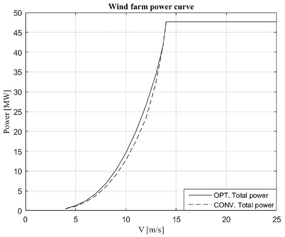
Power curve of the wind farm, conventional scheme (CONV.) versus present scheme (OPT.).
Wind turbine level
We conducted a case study to demonstrate the performance of the designed wind turbine control scheme to track the supervisory level commands. The study considered a wind farm with an initial wind speed of 12 m/s, similar to the conditions in case 2 of section B, where the wind turbines operate in two distinct regions of the power curve. We have shown the performance of turbines 1, 4, and 7 in the same column of the wind farm, as shown in Figure 8.
To conduct the study, we assumed a constant wind speed of 12 m/s for 50 s, during which the supervisory controller determined the axial induction factors of each turbine based on the wind farm’s maximum extracted power. The results of the supervisory control are summarized in Table 9 in the previous section. We then changed the wind speed from 12to 14 m/s over 20 s, and the supervisory controller adjusted the axial induction factors of each turbine to maintain maximum power extraction. Figure 10 shows the axial induction factor and wind velocity for turbines 1, 4, and 7, as determined by the supervisory controller.
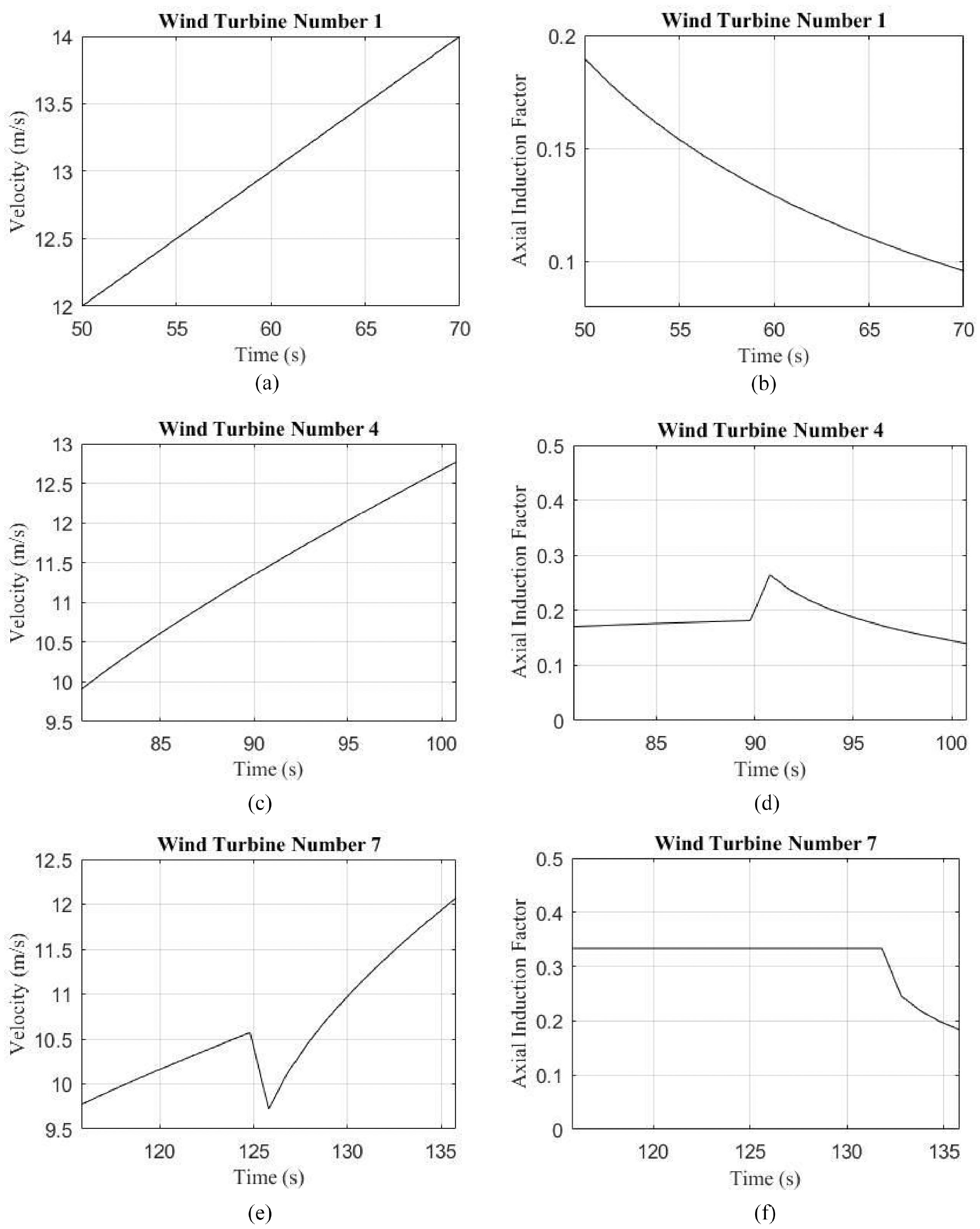
Axial induction factor and velocity of wind turbine number 1, 4, and 7 from supervisory controller: (a), (c), and (e) The velocity in rotor of wind turbines number 1, 4, and 7 respectively. (b), (d), and (f) The axial induction factors of these turbines which are calculated through the optimization algorithm.
As shown in Figure 10(a), in different wind velocities (from 12 to 14 m/s), wind turbine number 1 has operated in full load region where the extracted power is constat and equal to rated one. Therefore by the increment of wind velocity, the axial induction factor has decreased, and more portion of wind power has fallen on the second-row wind turbine, number 4. As evidence, besides the wind velocity at the front row had a 17% increment (from 12 to 14 m/s), at the second row, we see about a 29% increment (from 9.91 to 12.76 m/s). The difference between the timelines of wind varies in the three wind farm rows because of the time required for the wind to travel from the front row to the downstream rows. As illustrated in Figure 10(d), wind turbine number 4 operated in the partial load region until the second 90, and after that, with a transition, it transferred to the full load region. In the full load region, the axial induction factor has decreased with the increment of wind velocity. The sharp rise of wind velocity at wind turbine number 7 (Figure 10(e)) is due to the that the upper wind turbine (number 4) transferred to the full load region, and therefore more portion of wind power (and consequently velocity) has fallen at the downstream one. Figure 10(f) also shows that wind turbine number 7 operated with an axial induction factor equal to 0.33 in the partial load region, and by the increment of wind velocity, it also has transferred to the full load region of the wind turbine power curve. The value of the axial induction factor in partial load is equal to 0.33 because wind turbine number 7 is the last row, and its wakes and effects on the downstream are not important to us, and we want to extract the maximum power from the wind. Previously, it has been mentioned that for maximum power point tracking, the axial induction factor should be equal to 0.33.
In order to illustrate the ability of the proposed control system to attenuate the initial conditions and disturbances, we assume that the initial generator angular speeds in all wind turbines in the following simulations are 80 rad/s which is different from its rated value. The simulation results are presented in Figures 11 and 12.
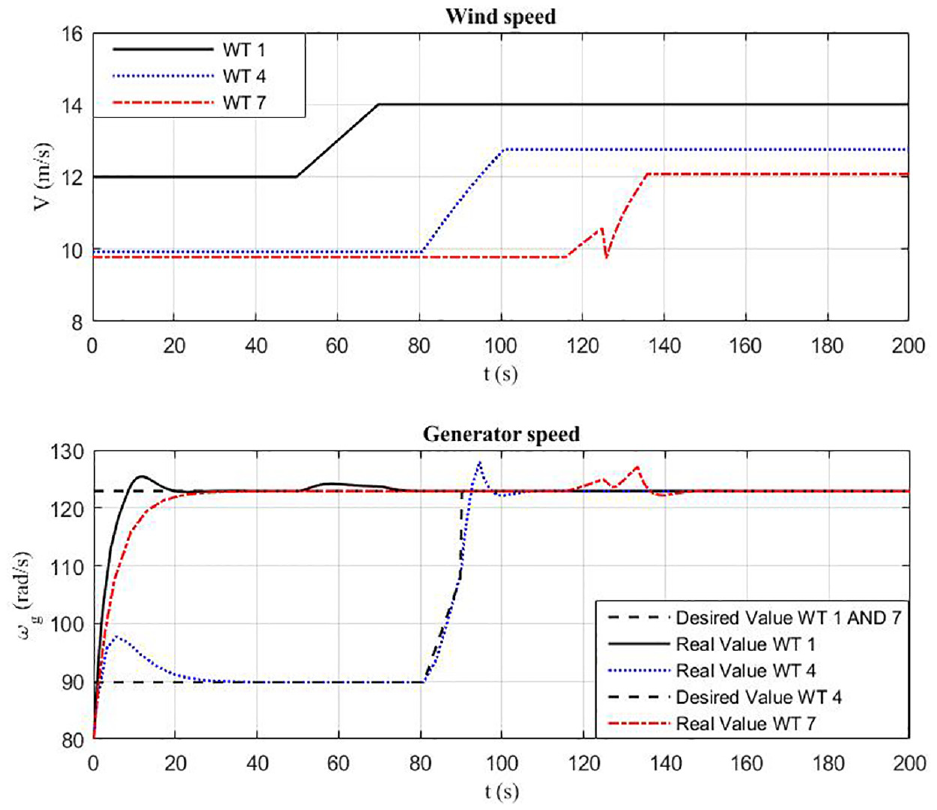
The wind turbine 1, 4, and 7 generator speed under the proposed controller when wind speed changes from 12 to 14 m/s.
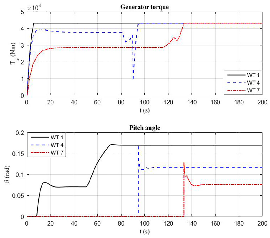
The wind turbine 1, 4, and 7 blades’ pitch angle and generator’s torque under the proposed controller when wind speed changes from 12 to 14 m/s.
Wind turbine 1
Wind turbine number 1 works in its full load region, and increasing velocity does not affect the power output. Since the turbine is working in its full load region, the pitch angel should tune as controller commands while the generator torque will stay at its maximum value (Figure 12). As mentioned before, the initial generator angular speed is 80 rad/s, and the wind turbine started in the partial load region. Therefore, at the beginning of the operation, generator torque is employed to control the generator’s angular speed. Less than about 25 s later, the generator angular speed settles on its rated value and keeps constant until t = 50 s when wind velocity change is encountered. It is shown in Figure 11 that the controller well decays the wind speed change effects and keeps the generator angular speed at the rated value.
Wind turbine 4
Wind turbine 4 operates in the partial load at the beginning, but it transfers to its full load region by increasing wind velocity. Increasing the free stream wind velocity from 12 to 14 m/s causes local wind velocity increment from 9.91 to 12.76 m/s in the wind farm’s second row and change in the corresponding wind turbines operation regions.
Operation regions of the power curve are the key points of the proposed controller. As presented in Figures 11 and 12, when the turbine operates in its partial load region, the generator torque is implemented to control the system. By increasing the wind velocity, the operational region transfers from partial load to full load region. The pitch angle is used in the full load region to control the wind turbine system. However, as velocity increases, there is a point that the controller switches between using generator torque or pitch angle. This point is obviously shown in Figures 11 and 12. Since the velocity reaches its rated value while the generator torque does not reach its maximum value, the switching between generator torque and blades pitch angle control schemes does not occur. This condition defines as a transient region between partial load and full load region in which the generator speed reaches its rated value, but the generator torque is below its maximum value. In this condition, generator torque is used to keep the generator speed constant at its rated value while the pitch angle remains zero.
Wind turbine 7
This wind turbine is located at the last row of the wind farm; thus, its control strategy is to capture as maximum power as possible from wind. Therefore, the turbines’ axial induction factors located in the wind farm’s last row will be tuned at their maximum values. For this purpose, the internal control loop sets the pitch angle to its optimum value in the partial load region (set to zero) and uses the generator torque to control the wind turbine. Increasing the free stream wind velocity from 12 to 14 m/s causes local wind velocity increment from 9.77 to 12.07 m/s in the last row of the wind farm and a change in the corresponding wind turbines operation regions.
Wind turbine 7 operates in a region where the generator speed is set to the maximum, but the generator torque does not reach its maximum value. This condition is the transient region between the power curve’s partial load and full load regions. In this condition, generator torque is used for controlling the system, and the pitch angle remains zero until the region change occurs.
In this simulation scenario, wind turbine 4 operates in the transient region for just a few seconds, but wind turbine 7 operates in the transient region for all times of simulation before transfer to its full load region. This difference between these two turbines stems from the different axial induction factors calculated by the supervisory controller. Wind turbine 7 operates at its maximum axial induction factor value (a = 0.333), which causes it to have maximum generator speed in lower wind velocity compared to wind turbine number 4, which operates at an axial induction factor of a < 0.333.
Conclusion
In conventional wind farm control, all wind turbines are set individually to extract maximum power. This setting doesn’t guarantee maximum power extraction from the whole wind farm. Because the high axial induction factor in upstream wind turbines reduces the power output of downstream wind turbines. In this paper, an axial-induction-based model was utilized to predict the wind velocity distribution in the wind farm. Analytical dynamics and aerodynamics of wind turbines in conjunction with the aforementioned wake model are implemented to simulate the wind flow and interactions among wind turbines in the wind farm. The main idea of this research is to take into account the effect of wake flow and flow interactions in optimizing the whole wind farm power output. In this regard, two cascade control loops are considered, including supervisory and internal control loops. In the supervisory control loop, the genetic algorithm has been used to optimize the whole wind farm output power by setting each turbine axial induction factor. In the internal control loop, a comprehensive control is considered to guarantee the following of supervisory level command in the partial load region and the rated generator toque and speed in transient and full load regions.
The efficiency of the proposed control strategy is investigated using an example 3 × 3 wind farm layout. Simulation results demonstrate the satisfactory performance of the supervisory controller in the optimization of wind turbines’ set points. In addition, the results show the performance of the internal controllers at each wind turbine to follow up the aforementioned set points. Similar to the wind turbine power curve, the wind farm power curve was also introduced to show the power output enhancement of the proposed wind farm control in comparison to the conventional one. Based on the depicted results, it could improve power production by about 13.95%.
Footnotes
Declaration of conflicting interests
The author(s) declared no potential conflicts of interest with respect to the research, authorship, and/or publication of this article.
Funding
The author(s) received no financial support for the research, authorship, and/or publication of this article.