
Abstract
Rolling bearing is one of the core components in rotating machinery, and its running status directly affects the operation of the whole equipment. Faults of rolling bearings in the actual working process are often multiple faults. To effectively separate fault sources, the blind source separation method is used for the compound fault diagnosis of rolling bearings. Because of the impact of the number of artificially limited decompositions and quadratic penalty factor on VMD in the decomposition process, and the slow convergence and low accuracy in the objective function of traditional FastICA operation, the VMD algorithm based on the energy loss coefficient and the information entropy is proposed, which adaptively determines the number of modal components and the quadratic penalty factor; The Tukey M estimation is selected as the objective convergence function of the FastICA algorithm to improve its robustness. First, VMD is used to decompose the signal; Secondly, the original signal and the decomposed IMF component are reconstructed, the covariance matrix and the singular value decomposition are constructed, the number of fault sources is estimated by the proximity dominance method, and the decomposed IMF components are filtered through correlation analysis and kurtosis index to build a multi-channel feature set; Finally, the constructed multi-channel feature set is input to the FastICA algorithm based on the Tukey M estimation for the separation of fault source signals to achieve composite fault diagnosis. The compound fault experiment shows that the proposed method in this paper can effectively realize the blind source separation of rolling bearing fault features to realize the compound fault diagnosis in different positions.
Keywords
Introduction
Rolling bearing is one of the most widely used components in modern industrial equipment, its running state directly affects the performance of the entire kit, so it is essential to conduct relevant research on bearing fault diagnosis technologies. However, in practical work, once the rolling bearing is damaged, it may not only be a fault at one location but also a composite fault with multiple faults, signal frequencies of this fault are mixed, and multiple fault characteristics are superimposed and interfered with each other, making the fault characteristics complex and causing obstacles for fault diagnosis.
The traditional single-fault diagnosis method cannot accurately diagnose the compound fault. Therefore, many scholars have conducted in-depth research on problems of compound fault diagnosis. Li et al. 1 proposed a differential empirical modal decomposition (DEMD) based on the empirical modal decomposition (EMD) signal decomposition, and proved experimentally that the method could achieve better diagnosis of dual composite faults of the rotor. Jiang et al. 2 used the wavelet transform to decompose the original signal into different modes and finally used the Duffing oscillator theory to establish the separation model to identify different fault models. Li et al. 3 proposed the local mean decomposition, which solves the problem of mutual inclusion and coupling between signals by extracting the multi-scale energy entropy features of signals. At present, most of research in composite fault diagnosis focus on analyzing and dividing the frequency band. With the emergence of blind source separation technology, it provides a new way for researchers to solve the problem.
Blind Source Separation 4 (BSS) is an effective method to solve the problem of compound faults superimposed on each other and difficulties of feature extraction compared to single fault diagnosis, and it is a technique that can extract individual signals from mixed signals. Aliniya and Keyvanpour 5 first introduced the concept of Independent Component Analysis (ICA) for source signal recovery. Merola and Chen 6 were able to effectively eliminate noises and reduce the dimensionality of the sparse data using principal component analysis techniques, which also recovered the source signal better. Senguler et al. 7 used FastICA in conjunction with wavelet packet decomposition techniques. Wu et al.8,9 completed early fault diagnosis of rolling bearings by combining continuous wavelet transform with ICA. Yang and An10–14 proposed a method to apply Empirical Mode Decomposition (EMD) and ICA to extract weak tomographic signal features from bearing vibration signals.
The multi-channel blind source separation technology is relatively mature, and the single-channel blind source separation (SCBSS) technology is relatively late, which makes the conventional blind source separation algorithm subject to certain restrictions. The precondition for the traditional blind source separation algorithm application is that the number of observed signals is not less than the number of source signals. In the actual signal acquisition process, due to the lack of known information, it is often in the underdetermined state. The single-channel blind source separation problem is a special case of underdetermined blind source separation. In this case, it is tough to use BSS to achieve the correct signal separation. With the emergence of signal decomposition techniques, it also provides new ideas for single-channel blind source separation techniques. The single-channel signal can be decomposed into multi-channel signals by new tools such as wavelet transform, 15 local mean decomposition (LMD) and empirical mode decomposition (EMD). Hong and Liang 16 combined wavelet transforms with the ICA algorithm to achieve an accurately diagnosis of compound faults from the single-channel acquisition. Deng et al. 17 used the full-set ensemble empirical modal decomposition combined with the FastICA algorithm to achieve better separation of fault source signals from the single-channel acquisition. Shi et al.18–22 proposed a gearbox fault diagnosis method based on EEMD and single-channel blind source separation, and verified the feasibility of the method through experiments. Wu et al. 23 used wavelet decomposition to obtain a series of high-frequency signals to form multi-channel signals, and used the ICA method to achieve BSS. However, all of the above methods have shortcomings. In wavelet decomposition, different wavelet bases and decomposition layers will get differences in detailed signals and approximate signals, which will affect the signal separation effect. When EMD is used to decompose signals, modal aliasing will occur. The EEMD decomposition method suppresses the modal aliasing problem to a certain extent, but it brings issues such as the increase in the number of IMFs and the long-time consuming algorithm. Many problems in engineering can be transformed into optimization issues.24–27 ICA can take too long to train due to its own optimization issues. FastICA (Fast Independent Component Analysis) is a fast convergence algorithm with a high separation accuracy in independent component analysis. The traditional gradient finding algorithm has limitations and is susceptible to step size selection, which can affect the final separation result. FastICA does not involve the selection of parameters such as step size, which will make the convergence speed fast. But the robustness of the estimation is poor, and it is sensitive to the initial value, which will affect the accuracy of composite fault diagnosis.
In response to the above problems, a new rolling bearing composite fault diagnosis method is proposed. The method utilizes the advantages of VMD decomposition method and FastICA method based on Tukey M estimation to separate the composite fault signals. The proposed method is named the single-channel blind source separation based on VMD and Tukey M estimation. The method based on improved VMD can effectively decompose the original signal and overcome the problem of modal aliasing in signal decomposition such as EMD and EEMD. Using Tukey M estimation as the second-order continuous derivable function of negative entropy calculation can reduce the impact of individual residual values on the least squares estimation results, thus further improving the convergence speed and robustness, and overcoming the problems of FastICA algorithm. Firstly, VMD is used to decompose the signal after wavelet packet adaptive threshold denoising, and a method is proposed to determine the number of VMD decomposition layers and quadratic penalty factor based on energy loss coefficient and information entropy; Secondly, the original signal and the decomposed IMF components are reconstructed, the covariance matrix is constructed, the number of fault sources is estimated using the proximity dominance method, and the correlation and kurtosis indicators are used to filter the fault source characteristics; Finally, the filtered IMF components are input into the FastICA fault diagnosis model based on Tukey M estimation to achieve fault source signal separation. The experimental results show that the method proposed in this paper can effectively overcome the problems such as modal confusion arising from traditional signal decomposition, improve the convergence speed and robustness of FastICA algorithm, realize the separation of bearing composite fault signals, and diagnose and identify the bearing composite faults. The main contributions of this paper are as follows:
(1) An improved feature dimension raising method for VMD is proposed. Based on the energy loss coefficient and the information entropy, the number of modal components and the quadratic penalty factor is determined adaptively, the number of fault sources is estimated according to the proximity dominance value method, and different features are filtered by using the correlation and kurtosis indexes to effectively achieve the feature dimension raising.
(2) A FastICA blind source separation method based on Tukey M estimation is proposed to improve the accuracy of fault diagnosis.
(3) The effectiveness of the method is verified by public data sets and experimental data, and compared with other algorithms to prove that the proposed method in this paper can better separate the fault signals.
The rest of this paper is organized as follows. Section II mainly introduces the basic theory about raising the feature dimension of the original signal by using VMD, and constructing a multi-channel feature set as the input of the blind source separation algorithm. Section III presents the FastICA blind source separation method based on the Tukey M estimation, and describes in detail the specific process of fault diagnosis using the proposed method in this paper. Then, in section IV, the proposed method is verified through public data sets and experimental data, and compared with KL-ICA and VMD-FastICA algorithms, proving that the proposed algorithm is more advantageous. Finally, section V concludes this paper and prospects for future work.
Feature lifting for adaptive variational modal decomposition
VMD decomposition
The VMD 28 is a variational problem constructed on the original signal, which is solved by the iterative computation and the introduction of the Wiener filtering to determine the center frequency of each eigenmode component as well as the bandwidth. The VMD solution process consists of two main constraints: (1) the sum of the bandwidths of the center frequencies of each modal component is required to be minimized; (2) the sum of all modal components is equal to the original signal.
VMD decomposes the original signal x(t) into several IMF component signals uk(t). Each IMF component regards it as a group of AM and FM signals. Hilbert transform each IMF component to obtain its unilateral spectrum
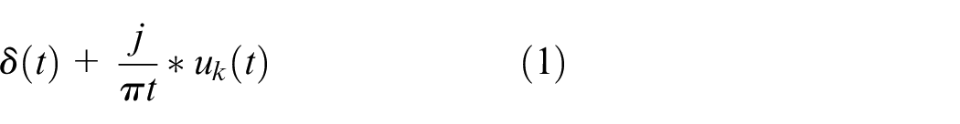
In the formula, δ(t) is the unit impulse function, * is the convolution operation, and j is the imaginary unit;
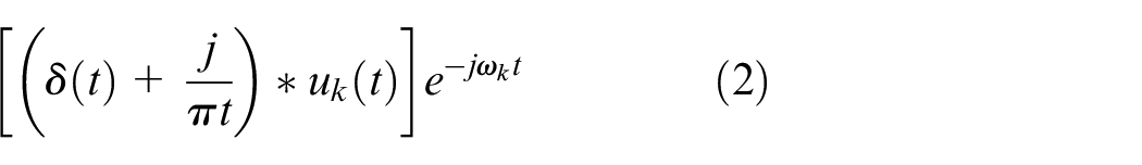
Through exponential correction, its unilateral spectrum is transferred to the baseband
Then, the gradient of the modulated signal is calculated by the square of L2 the norm to construct the variational problem
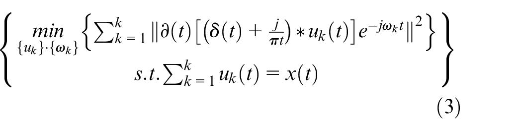
where uk(t) is the set of IMF components obtained by decomposition
Converting the constrained variational problem into an unconstrained variational problem by introducing Lagrange multipliers and quadratic penalty factors on the basis of equation (3), the transformation results
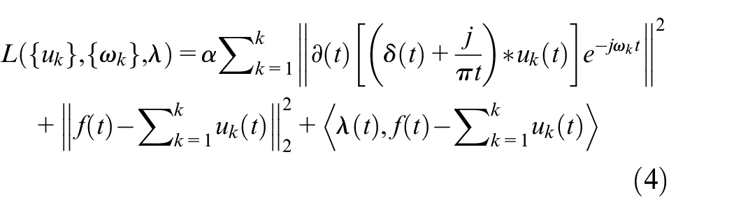
In the formula, λ is the Lagrange multiplier, and α is the quadratic penalty factor.
Finally, the main variable
Update formula for the modal component un+1K
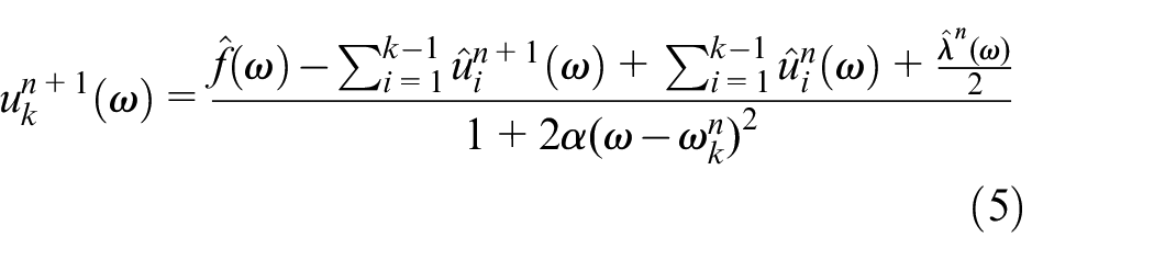
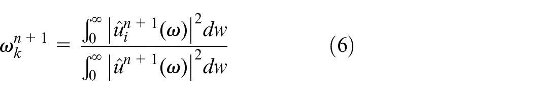
Update formula for central frequency ωn+1 k
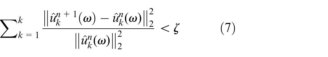
Using the above equation, the iterative update of un+1 K , ωn+1 k is continuously iterated and the termination condition of the iteration
Adaptive parameter determination
VMD involves two critical parameters 29 in the signal decomposition process, and the number of decomposition layers k and the quadratic penalty factor α need to be set in advance before the signal is decomposed. If the number of decomposition layers is set too low, it will be inadequate decomposition of the signal; if the number of layers of signal decomposition is set too high, it will result in redundancy of the individual modal information. The larger the penalty factor and the narrower the bandwidth of the resulting modal component, the smaller the penalty factor, the larger the bandwidth of the decomposed modal component. In this paper, an improved adaptive VMD algorithm is proposed based on the adaptive determination of the number of modal decompositions using energy loss coefficients before the VMD decomposition based on the energy relationship between the decomposed signal and the original signal. The energy loss factor is defined as the difference between the energy of the decomposition residual and the ratio of the energy of the original signal and is calculated as
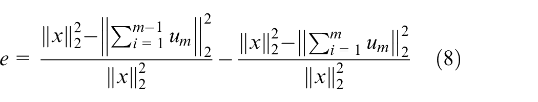
where x is the original signal, u k is the eigenmodal component and e is the energy loss coefficient.
The VMD decomposition is deemed complete when the energy loss coefficient e reaches a set threshold ε. 30 When the number of VMD decompositions is determined, the calculation of the information entropy is introduced and the quadratic penalty factor is determined.
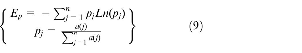
In the formula,
Information entropy mainly reflects the uncertainty of the system. When the rolling bearing failure occurs, it will produce periodic uniform pulse shock. When the signal is considered to be ordered, the information entropy value is relatively small. The IMF component of the VMD decomposition will contain fault information, and the VMD decomposition is considered complete when the information entropy value reaches a minimum.
Source number estimation and screening of high-quality IMF fractions
Once a bearing has failed, the number of sources of failure is often not determined, and this paper relies on the method of proximity dominance to estimate the number of sources of failure. After the VMD decomposition to obtain k IMF components, the original signal is formed into a new feature matrix with k IMF components ximf = [x (t), u1 (t), u2 (t) ……uk (t)], Construction of the covariance matrix Rimf = [ximf(t), xTimf(t)], and perform the singular value decomposition to obtain the eigenvalue matrix [λ1, λ2, λ3 …… λk], eigenvalues are then arranged in descending order, and the ratio between two adjacent eigenvalues is found Δ = λ1/λ2
The number of source signals is determined by the maximum ratio between adjacent eigenvalues.
The VMD decomposition yields k IMF components, which need to be filtered to exclude spurious components. This paper uses principles based on the number of interrelationships and the selection of the kurtosis index to screen for valid IMF components. The number of interrelationships directly represent the degree of similarity to the original signal, and the kurtosis index can better characterize the bearing failure shock characteristics. The screened IMF components are used to construct a multi-channel feature set as input to the blind source separation algorithm.
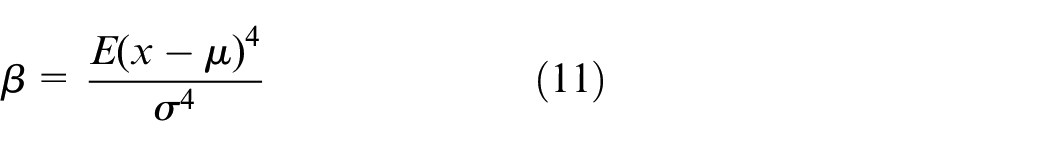
The formula for kurtosis is
The cross-correlation coefficient is calculated as
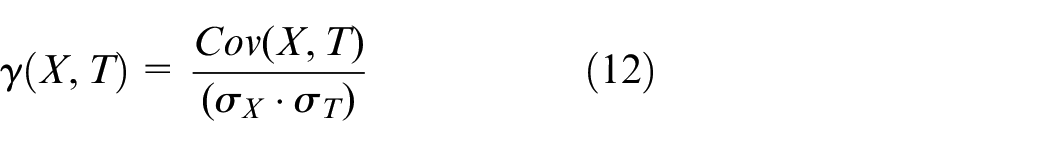
In formulas (11) and (12), E is the mathematical expectation,
Blind source separation of FastICA based on Tukey M estimation
Single-channel blind source separation
The blind source separation solution process makes three assumptions: (1) each source signal xm must be independent of each other; (2) the number of observed signals must be greater than the number of source signals; and (3) the mixing matrix column is full rank. None of these three conditions can solve the blind source separation problem if one is missing. Depending on the relationship between the number of sensors and the number of fault sources, they are classified as positive, underdetermined and overdetermined blind source separation. In the actual rolling bearing work process, due to the constraints of actual conditions, often the number of sensors will be smaller than the number of fault sources, belonging to the underdetermined blind source separation problem. This paper investigates the particular case of the underdetermined blind source separation process, the single-channel blind source separation problem, where the recovery of the faulty source signal is achieved by collecting the signal through only one channel with relatively less known information.
Single-channel blind source separation model
Where y(t) is the signal collected by a single channel, xi is the signal from multiple fault sources, and ai is the mixing matrix coefficient.
This paper uses the virtual channel method to solve the problem of requiring the number of observed signals to be greater than or equal to the number of fault source signals. The virtual channel method is the process of converting a single channel signal into multiple virtual channel signals through signal processing, which varies to increase the known signal. In this paper, we mainly use the variational modal decomposition to decompose the single channel signal into multiple virtual channel signals, which can better overcome the modal mixing problem, and finally achieve the feature separation of the signal by FastICA with Tukey-M estimation.
FastICA algorithm based on Tukey M estimation
When the ICA model is used to process mixed signals, it is necessary to perform pre-processing operations such as averaging and whitening. The objective function of the ICA algorithm and the selection of the optimization algorithm will directly affect the final separation effect. The objective function mainly selects some independence metric functions, and the extreme value of the objective function is obtained so that the independence or non-Gaussianity of the target signal can be maximized. Common independence metric functions mainly include the likelihood function, the non-Gaussianity metric and the mutual information related constraint function. The non-Gaussianity metric mainly consists of two kinds based on negative entropy and cliff metrics.
FastICA has advantages of faster convergence and higher separation accuracy. It does not involve selecting parameters such as the step size and the convergence, which is a fast and stable algorithm. The selection of the FastICA objective function will also directly affect the final separation effect. This section introduces the negative entropy-based non-Gaussianity measure. The larger the negative entropy, the larger the non-Gaussianity, so the FastICA algorithm based on negative entropy maximization focuses on finding a matrix
Negative entropy can be expressed as

Where ygauss is the Gaussian signal and y is the observed signal, both have the same variance. H(•) is the differential entropy, which represents the expectation of a continuous random variable
When two signals have the same variance, the signal that obeys the Gaussian distribution has the highest entropy value. In practice, it is not possible to obtain a probability density distribution of a vibrational signal that can be solved for negentropy in differential entropy form. Negative entropy can be approximated by expressing

Where E[•] is the mathematical expectation and G[•] is an arbitrary second-order continuous derivative function, where the choice of G[•] directly affects the final separation. g[•] is the derivative of G[•]. A common G[•] function contains the following three

Where a1 is a constant, chosen in the range,1,2 usually the value of a is chosen as 1; G3(y) is an expression for the kurtosis, the separation effect on G1(y) and G2(y) is a little better.
The FastICA algorithm constructs the Lagrangian equations by introducing Lagrangian factors and solving the Jacobian matrix using Newton iteration, and the iterative results are obtained as shown below.

The steps of FastICA algorithm based on negative entropy are as follows:
(1) Data pre-processing (averaging, whitening) of the observed signal x;
(2) Set the number of separated signals k;
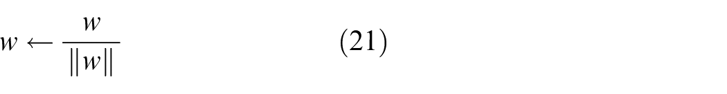
(3) Randomly initialize the matrix w, and the norm is equal to 1;
(4) Iteration
(5) Determine whether
(6) Output the estimated signal.
In this paper, the Tukey M estimate is chosen as the second-order continuously derivable function for the (G[•]) negative entropy calculation. Tukey M-based estimation can better solve the problem of the least squares estimation, which is susceptible to the influence of some large residuals when performing least-squares estimation. Tukey M-based estimation can internally assign a small weight to hefty residuals and a large weight to small residuals, thus significantly reducing the influence of individual residuals on the estimation results, and the Tukey M-based estimation improves the robustness of the estimation to some extent.
The specific expression for the Tukey M estimate is
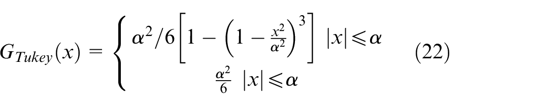
Where α is the threshold value, mainly to address the impact due to outliers in the estimation, based on statistical regression analysis, usually α is taken as 4.68.
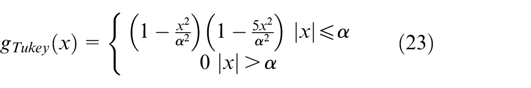
The second-order derivative
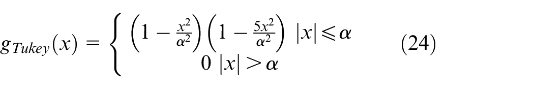
As can be seen from the first-order derivatives of which the second-order derivatives do not involve the associated complex operations of exponential, trigonometric and inverse trigonometric, the calculation process is relatively simple and faster compared to the traditional FastICA calculation.
Fault diagnosis process
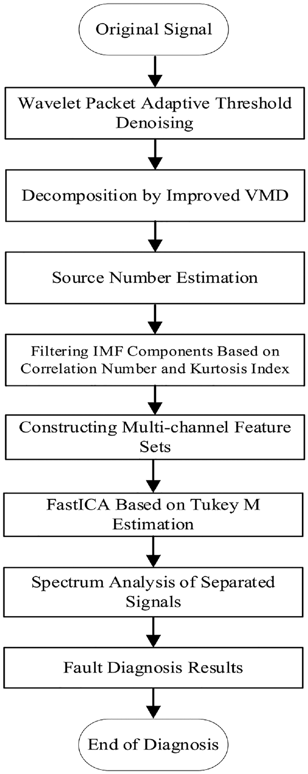
To realize the fault diagnosis of rolling bearings under the mutual coupling of multiple fault source signals, this paper proposes a single-channel blind source separation rolling bearing composite fault diagnosis method based on VMD and Tukey M estimation, which can accurately estimate the number of fault sources and overcome the modal mixing problem arising from the traditional signal decomposition, while improving the computational efficiency and the accuracy of fault diagnosis. The compound fault diagnosis process is shown in Figure 1. The specific blind source separation fault diagnosis framework is as follows:
(1) Adaptive threshold denoising of wavelet packets on the acquired signal, which can effectively filter out the high-frequency noise while retaining the feature information of low-frequency signals and signal integrity to the maximum extent;
(2) Determine the number of decomposition layers and the quadratic penalty factor using the energy loss coefficient and the information entropy, and implement the VMD decomposition;
(3) The decomposed IMF components and the original signal are formed into a new feature matrix, and the covariance matrix is constructed for the singular value decomposition to determine the number of source signals;
(4) The cross-correlation coefficient and kurtosis are used as indicators to screen IMF components, and IMF components with the same number of fault sources and the best indicators are selected;
(5) Build a multi-channel feature set with filtered IMF components
(6) Use the multi-channel feature set as the input of the blind source separation algorithm, and the feature set is separated by FastICA algorithm based on Tukey M estimation to recover the fault source signal and separate the fault features;
(7) Spectrum analysis of the separated signal to achieve composite fault diagnosis.
Fault diagnosis process.
Results and discussion
Public data verification
Using publicly available data from Case Western Reserve University, B021-2 fault data of drive end bearing roller and IR014-3 fault data of inner race are adopted. The fault frequency of inner race is 119.732Hz, and the fault frequency of roller is 92.341 Hz. The time domain and frequency domain of single fault signal are shown in Figures 2 and 3.
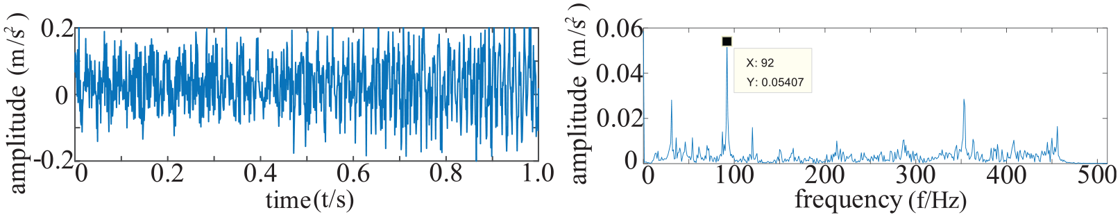
Rolling element fault signal waveform.
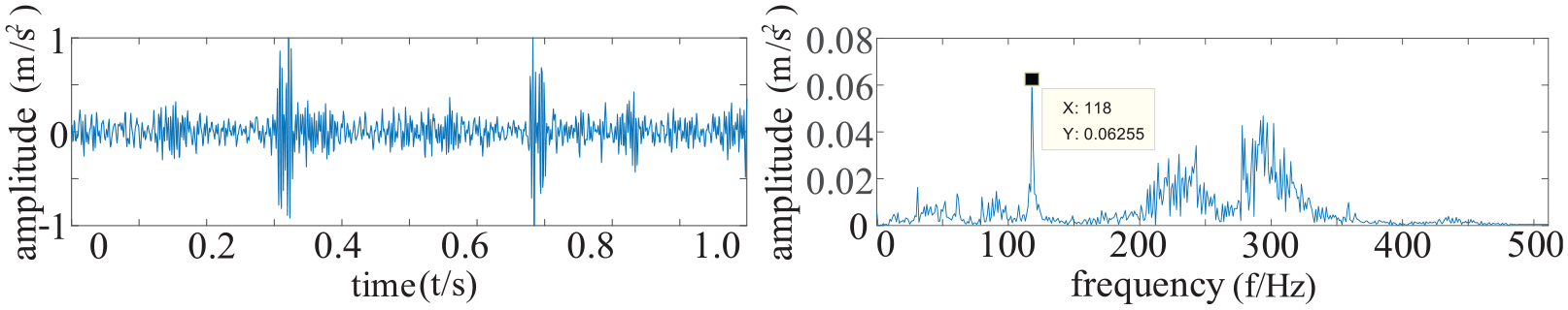
Inner ring fault signal waveform diagram.
Two single fault signals are mixed by the random matrix A = [1.58,1.32] to get the observation signal X. The time and frequency domain of the observation signal are shown in Figure 4.
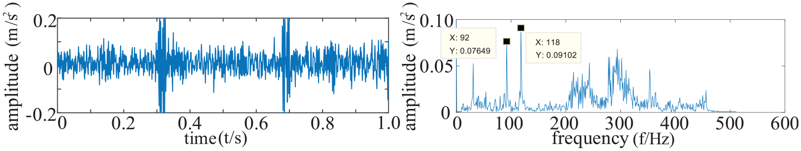
Complex fault signal waveform.
The wavelet packet adaptive thresholding is used to denoise the compound fault signal, and the denoised compound fault signal is processed with improved VMD to determine the complete signal decomposition when the number of decomposition modes is 5. The penalty factor is continuously changed, and the lowest information entropy is obtained when α = 1750. Determine the decomposition parameters k = 5, α = 1750, and decompose the signal to obtain the time domain frequency domain diagram shown in Figure 5.
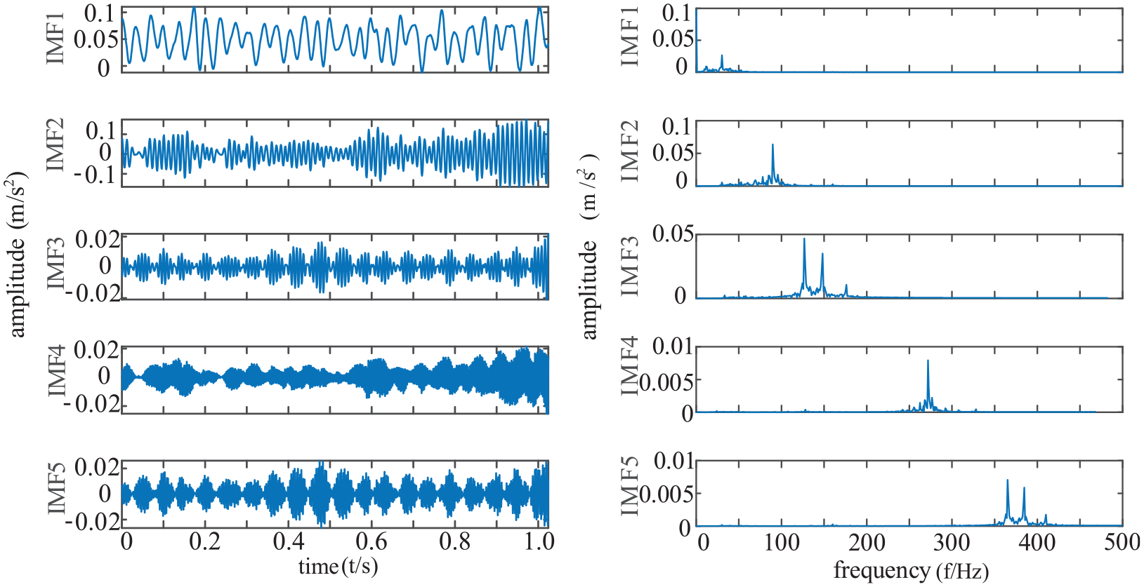
VMD signal decomposition waveform.
The original signal and the decomposed signal are reconstructed, the covariance matrix is constructed and the singular value is decomposed to obtain the individual eigenvalues. The ratio between adjacent eigenvalues is made to obtain the number of fault sources as 2, which is consistent with the actual number of fault sources. Based on the correlation and kurtosis indexes of the IMF components for screening, IMF2 and IMF3 were selected as high-quality components for the matrix reconstruction and used as blind source separation signal inputs. The filtered high-quality IMF components were input to KL-ICA and FastICA algorithms for comparison and analysis to obtain the results below.
As can be seen in Figure 6, the two fault impact frequencies after KL-ICA are not divided, the separation effect is poor, and there is a lot of high-frequency disorderly information. From Figure 7, it can be seen that the time domain signal after VMD-FastICA has some similarity with the original signal, and from the frequency domain plot it can be seen that the rolling body fault frequency 92.341Hz is separated out, but in the second frequency domain plot the inner ring fault frequency of 119.732Hz is not achieved a better separation, and it also contains the rolling body fault frequency. FastICA based on Tukey M estimation performs source signal recovery on the virtual multichannel signal obtained from VMD and obtains the blind source separation results, as shown in Figure 8.
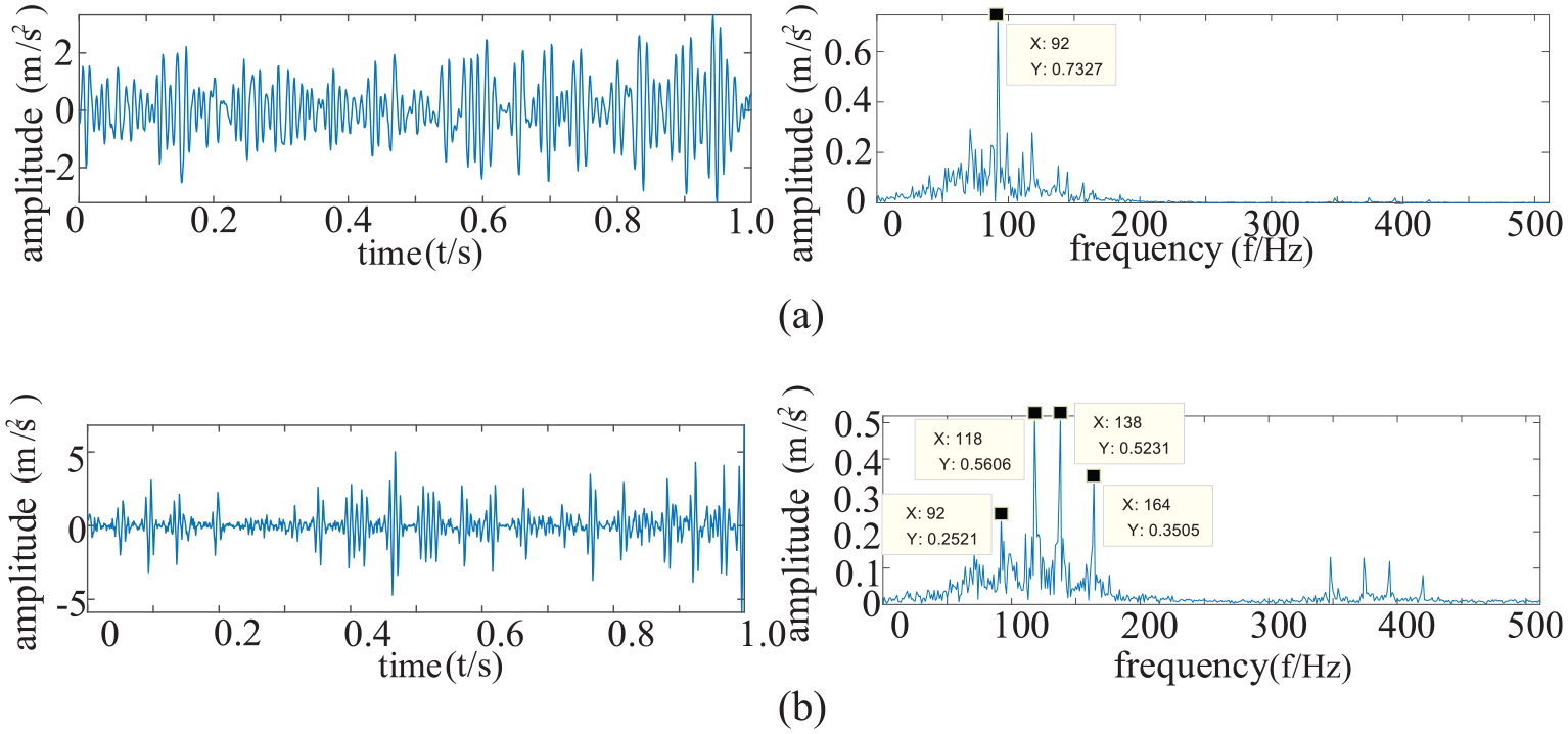
Time-frequency domain diagram after KL-ICA: (a) IMF2 time-frequency domain diagram and (b) IMF3 time-frequency domain diagram.
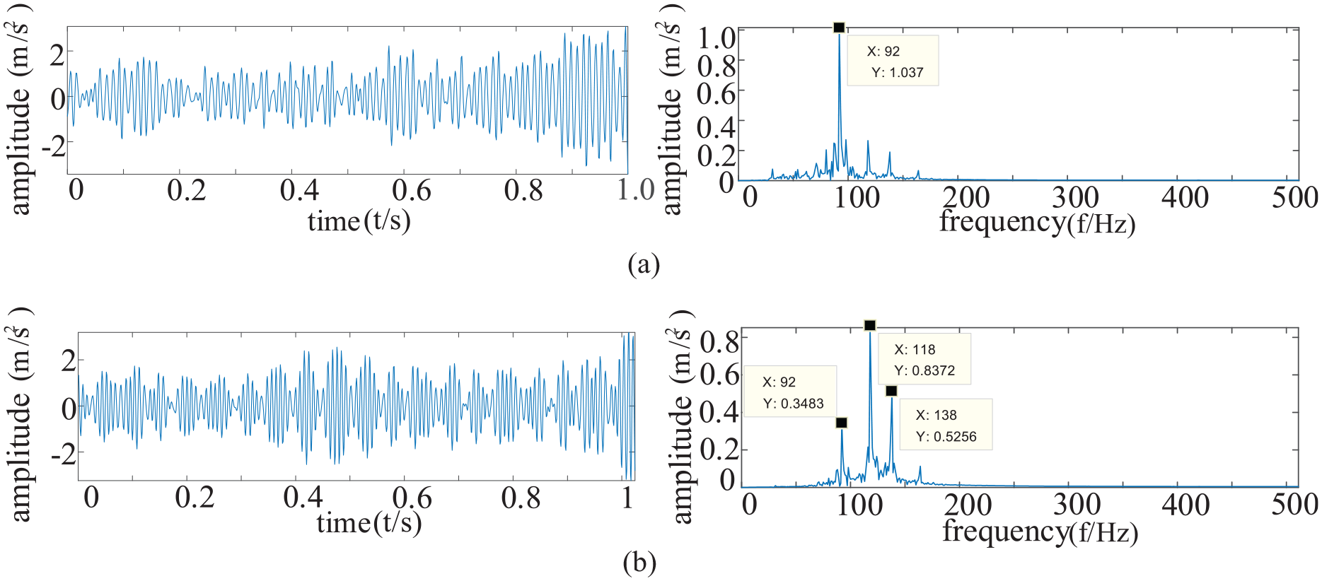
Time-frequency domain diagram after VMD-FastICA: (a) IMF2 time-frequency domain diagram and (b) IMF3 time-frequency domain diagram.
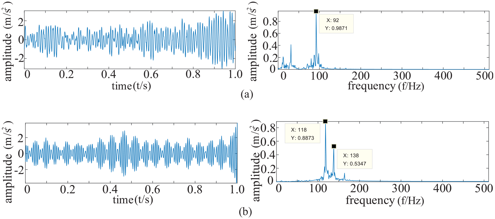
Time-frequency domain diagram after VMD-Tukey M-FastICA: (a) IMF2 time-frequency domain diagram and (b) IMF3 time-frequency domain diagram.
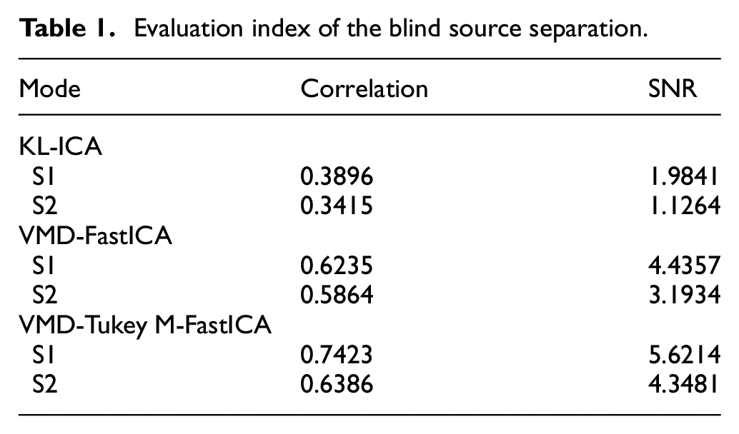
From the time domain diagram, it can be seen that the signal after the FastICA separation estimated by Tukey M has a high similarity with the original signal. The signal-to-noise ratio and the correlation analysis of the separated signals are shown in Table 1.
Evaluation index of the blind source separation.
Laboratory data verification
In this section, a single-row angular contact bearing failure simulation test is used to verify the effectiveness of the FastICA single-channel blind source separation method based on adaptive variational modal decomposition and Tukey-M estimation. The rolling bearing fault simulation test bench is shown in Figure 9.
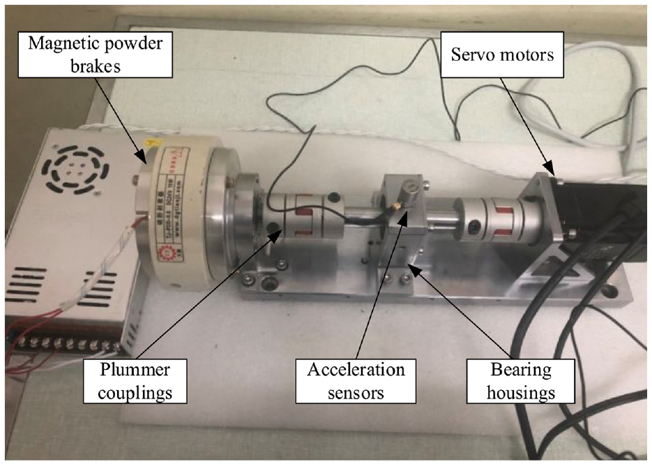
Rolling bearing fault simulation test bench.
The main components of the test bench are:
(1) YASKAWA/Yaskawa servo motor, rated voltage 200V, speed response frequency 3.1 kHz, rated power 0.1 kw, maximum speed 6000 r/min;
(2) CT1005LCICP/IEPE acceleration sensor, sensitivity 50 mv/g, frequency range 0.5–8000 Hz;
(3) TJ-POD-A magnetic powder brake, mass 0.6 kg, voltage 24 V, current 0.81 A, slip power 130W, maximum speed 1800 r/min, damping 1.35 lbs constant in the experiment;
(4) GFC coupling with elastic spider, nominal torque 12.5 N.m;
(5) Base and bearing seat, connections and fasteners.
The data acquisition system is the CoCo-80 Dynamic Signal Analyzer, as shown in Figure 10. The accuracy and performance of the device are at the front of the industry, and it also has advantages of low-cost, portable, battery-powered, and easy operation. The data is collected by the acceleration sensor and saved to the SD card of CoCo80. The data is imported into the computer from the SD card and converted into .mat files by the EDM software for further data processing.
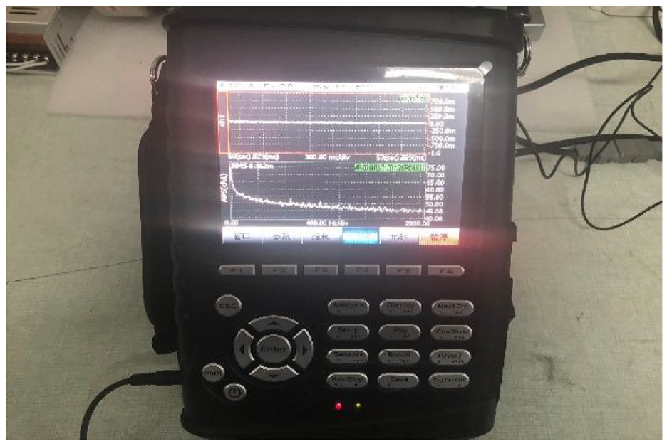
CoCo-80 data acquisition analyzer.
This paper mainly uses the rolling bearing outer ring and the rolling body compound fault data. Experiments refer to CWRU University’s experimental ideas through the EDM wire cutting of different positions of the bearing for certain damage, simulating bearing failure. The experimental speed is 2000 r/min, the sampling frequency is 1024 Hz, the theoretical rotational frequency is 33.33 Hz, the theoretical failure frequency of the rolling body is 77.186 Hz, and the failure frequency of the outer ring is 128.429 Hz. When the bearing operation is stable, from which two consecutive seconds of the stable operation are selected, the time domain frequency domain of the original data of the compound fault is shown in Figure 11.
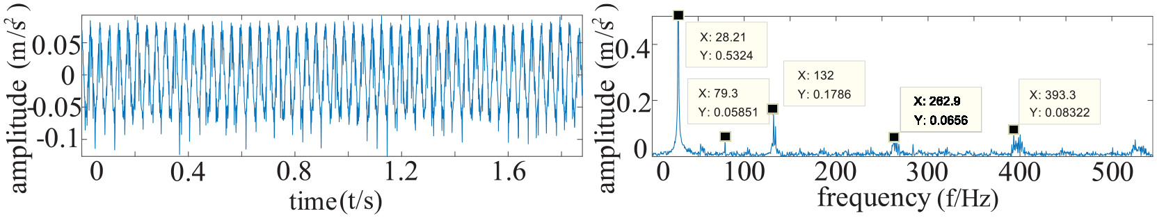
Compound fault vibration signal waveform diagram.
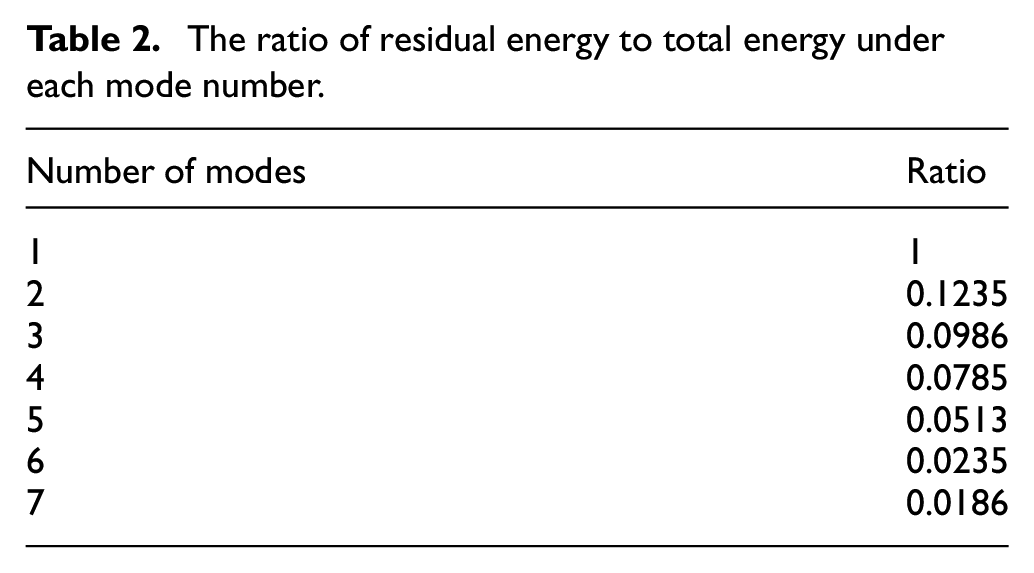
The bearing vibration signal is characteristically up-dimensioned by VMD, and the results of the ratio of residual energy to total energy Ei (i = 1, 2, 3) at each modal number are obtained based on the VMD decomposition as shown in Table 2.
The ratio of residual energy to total energy under each mode number.
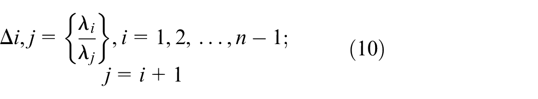
The energy convergence factor Δij(i = 1,2,3,…,N,j=i+1) calculated according to Formula 8 is shown in Table 3.
Difference of energy ratio between adjacent modes.
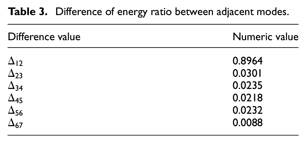
From the table, we can see that Δ67 < ε. It is considered that the signal decomposition is complete when the modal number is 6. Then the signal is decomposed based on the modal number of 6, the penalty factor is continuously changed, and the lowest information entropy is obtained when α = 1000. Determine the decomposition parameters k = 6, α = 1000, and decompose the signal to obtain the time-frequency domain diagram shown in Figure 12.
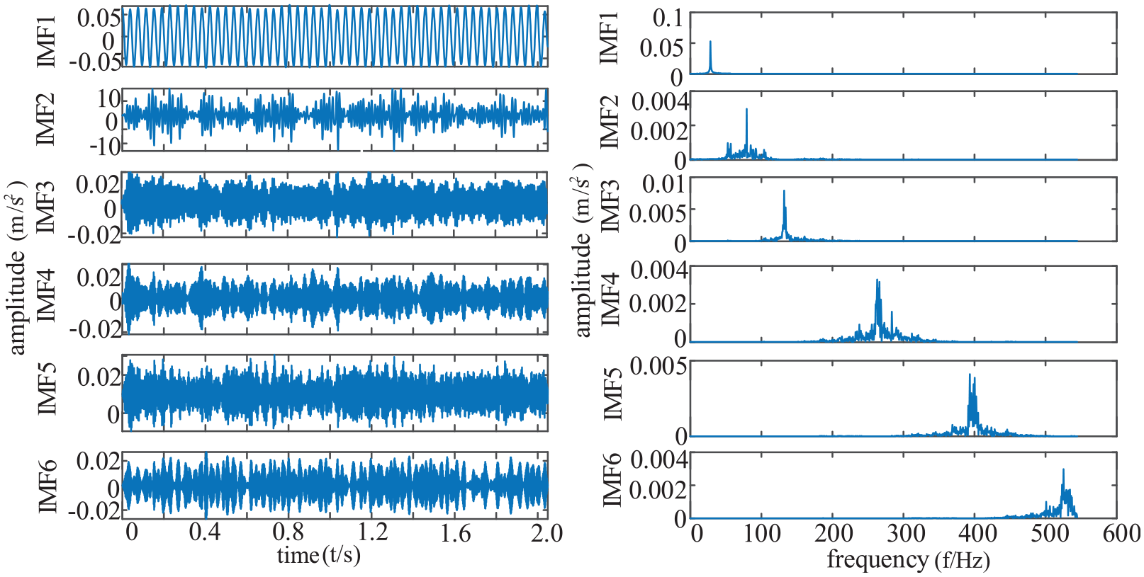
Time-frequency domain diagram of VMD signal decomposition.
The original signal and the decomposed signal are reconstructed, then the covariance matrix is constructed, and each of its eigenvalues is obtained by the singular value decomposition, and the ratio between adjacent eigenvalues is made to obtain the maximum Δ = 21.0784, which gives the number of fault sources as 2, which is consistent with the actual number of fault sources. Therefore, two optimal IMF components are selected from IMF components after the improved VMD decomposition for the matrix reconstruction. Their decomposed correlations for each IMF component and the kurtosis values are shown in Table 4.
Quality IMF component selection criteria for VMD decomposition.
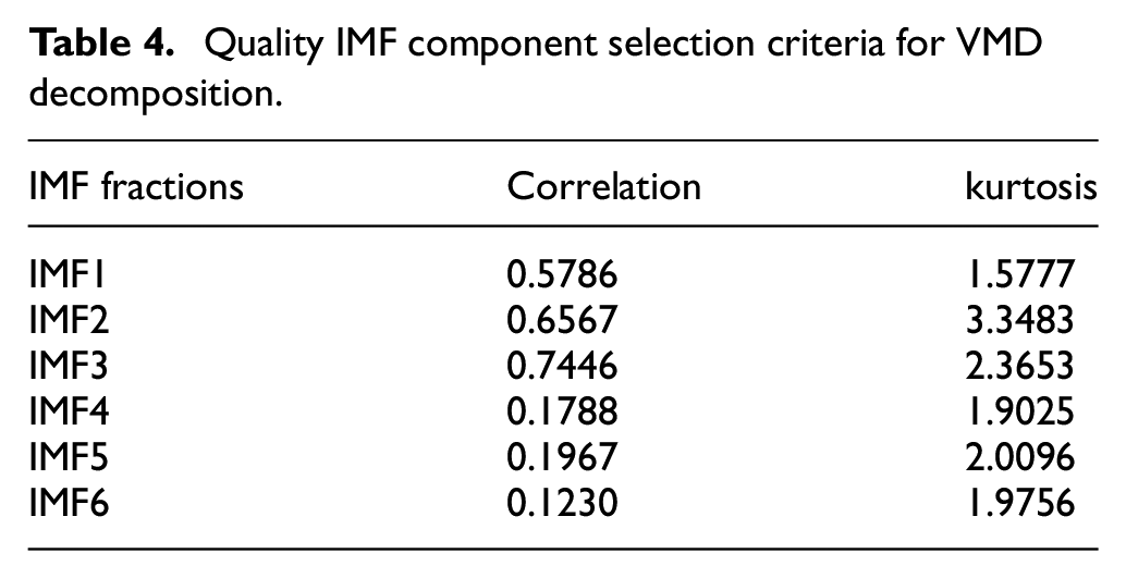
As can be seen in Table 4: the correlation between the second IMF component and the third IMF component is 0.6567 and 0.7446, respectively. And since two components including IMF2 and IMF3 have the greatest kurtosis, IMF2 and IMF3 are chosen as high-quality components for the matrix reconstruction technique. They are used as blind source separation signal inputs. After the Tukey M estimation based on the FastICA algorithm for the blind source separation of the reconstruction matrix, the recovery of the fault source signal, and the separation of fault features to achieve compound fault diagnosis, results are shown below.
As shown in Figures 13 and 14, the division of the failure frequency is not implemented. Only the rotating frequency is separated out. After VMD-FastICA separation, fault frequencies are not clearly divided. Compound fault frequencies contain each other, but the primary and secondary fault frequencies in each separated signal can be clearly seen. It can be seen from Figure 15(a) that the fault frequency separation effect of the VMD FastICA algorithm based on Tukey M estimation is good. The peak occurs at 28 Hz, which is close to the theoretical conversion frequency of 33.3 Hz, and the fault impact frequency of 79.3 Hz is close to the fault frequency of the rolling unit of 77.186 Hz. It can be judged that the rolling element of this bearing is faulty to a certain extent. It can be seen from Figure 15(b) that the oscillation impact occurs at 124 Hz, which is close to the theoretical fault frequency of the outer ring of 128.429 Hz. It also can be seen that the outer ring of the bearing is damaged to some extents. There is a certain error between the theoretical fault frequency and the actual fault frequency, but it can be within an acceptable range. This fully shows that the proposed method can effectively realize the blind source separation, the bearing compound fault diagnosis, and the recognition.
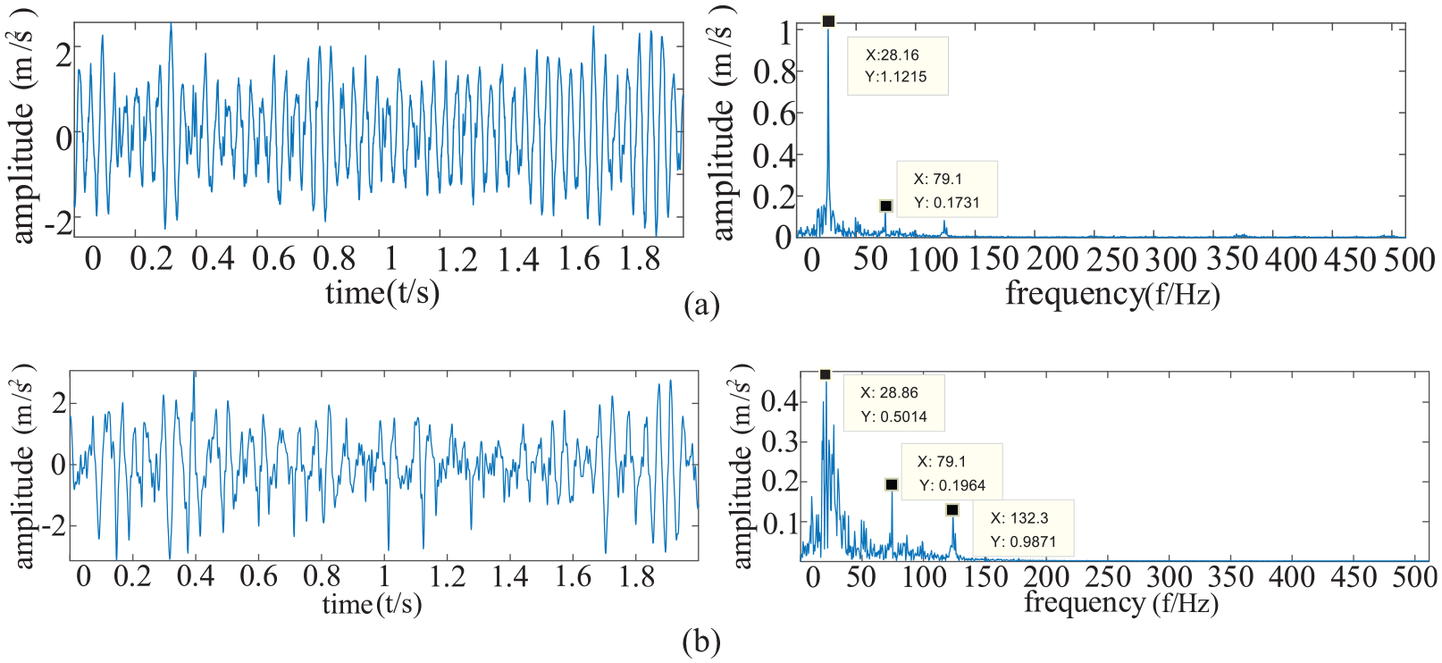
Blind source separation for KL-ICA: (a) IMF2 time-frequency domain diagram and (b) IMF3 time-frequency domain diagram.
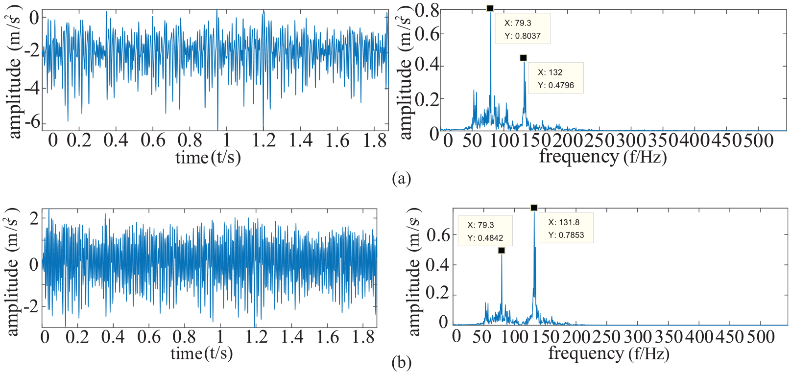
Blind source separation for VMD-FastICA: (a) IMF2 time-frequency domain diagram and (b) IMF3 time-frequency domain diagram.
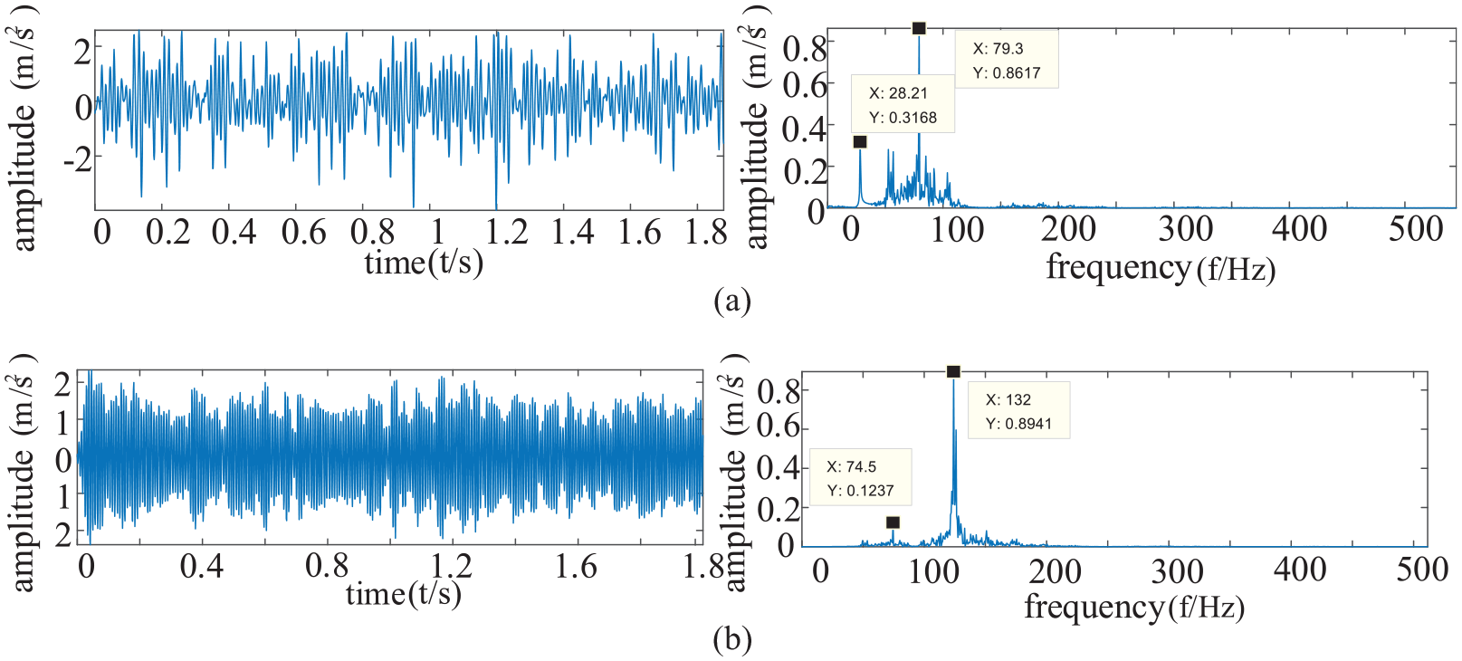
Blind source separation for VMD-Tukey M-FastICA: (a) IMF2 time-frequency domain diagram and (b) IMF3 time-frequency domain diagram.
Conclusion and future work
This paper proposes a single-channel blind source separation rolling bearing composite fault diagnosis method based on VMD and Tukey M estimation, which solves the problem that the previous single-channel blind source separation algorithm cannot recover the fault source signal accurately, and improves the accuracy of composite fault diagnosis. The feature dimension raising method based on the improved VMD can adaptively determine the number of decomposition and quadratic penalty factor, accurately estimate the number of fault sources, better divide the spectrum, and overcome the problem of modal aliasing. The FastICA algorithm based on Tukey M estimation is able to assign appropriate weights according to the size of the residuals, thus reducing the influence of individual residuals on the estimation results so as to improve its convergence speed and robustness. The method is verified by the public data set of Case Western Reserve University and the composite fault test bench, and compared with KL-ICA and VMD-FastICA algorithms. The improved blind source separation method in this paper has the largest correlation and signal-to-noise ratio between the separated signal and the original signal, which shows that the VMD-Tucky m-FastICA algorithm has better fault diagnosis accuracy.
The shortcoming of this paper is that the method has been experimentally validated only at low speed and stable operating conditions, and no relevant experiments have been conducted at high speed and variable operating conditions. In the future, the proposed method will be further improved and optimized, and the related research on composite fault diagnosis under high speed and variable operating conditions will be conducted.
Footnotes
Acknowledgements
The authors would like to thank Key Laboratory of Advanced Manufacturing Intelligent Technology of Ministry of Education for helpful discussions on topics related to this work. The authors are grateful to Ruofan Cao for his help with the preparation of figures in this paper.
Author contributions
Conceptualization, Wang.Y.P., Xu.D. and Zhang.Q.S; methodology, Wang.Y.P., Xu.D. and Zhang.Q.S; validation, Wang.Y.P., Xu.D. and Cao.R.F.; formal analysis, Wang.Y.P., Xu.D. and Cao.R.F.; investigation, Wang.Y.P., Xu.D. and Cao.R.F.; resources, Wang.Y.P., Xu.D. and Cao.R.F.; data curation, Wang.Y.P. and Cao.R.F.; writing—original draft preparation, Wang.Y.P. and Zhang.Q.S; writing—review and editing, Wang.Y.P. and Zhang.Q.S; visualization, Wang.Y.P. and Cao.R.F.; supervision, Wang.Y.P. and Cao.R.F.; project administration, Wang.Y.P. and Xu.D.; funding acquisition, Wang.Y.P. and Dai.Y.; All authors have read and agreed to the published version of the manuscript.
Declaration of conflicting interests
The author(s) declared no potential conflicts of interest with respect to the research, authorship, and/or publication of this article.
Funding
The author(s) disclosed receipt of the following financial support for the research, authorship, and/or publication of this article: This work was supported by the National Natural Science Foundation of China, grant number 52175502.
Data availability statement
Data is contained within the article.