
Abstract
Feature selection plays an important role in algorithms for processing high-dimensional data. Traditional pattern classification and information theory methods are widely applied to feature selection methods. However, traditional pattern classification methods such as Fisher Score, Laplacian Score, and relief use class labels inadequately. Previous information theory based feature selection methods such as MIFS ignore the intra-class to tight inter-class to sparse property of the samples. To address these problems, a feature selection algorithm for the binary classification problem is proposed, which is based on class label transformation using self-organizing mapping neural network (SOM) and cohesive hierarchical clustering. The algorithm first converts class labels without numerical meaning into numerical values that can participate in operations and retain classification information through class label mapping, and constitutes a two-dimensional vector from it and the attribute values to be judged. Then, these two-dimensional vectors are clustered by using SOM neural network and hierarchical clustering. Finally, evaluation function value is calculated, that is closely related to intra-cluster to tightness, inter-cluster separation, and division accuracy after clustering, and is used to evaluate the ability of alternative attributes to distinguish between classes. It is experimentally verified that the algorithm is robust and can effectively screen attributes with strong classification ability and improve the prediction performance of the classifier.
Introduction
With the development and application of information technology, more and more high-dimensional data such as: digital images, financial time series, and gene expression microarrays have been accumulated. Feature selection has become an indispensable pre-processing step in algorithms for processing high-dimensional data. Feature selection refers to the process of selecting a subset of features from all attributes that are most beneficial for subsequent operations to reduce the dimensionality of the feature space while keeping the decision-making capability of the information system unchanged. As an important part of knowledge discovery techniques, feature selection can improve the speed of knowledge learning, enhance the compactness of learning models, increase the generalization ability of models, 1 and enable one to utilize data with minimal complexity in order to improve the level of awareness of information implicitly contained in huge data.
Filter feature selection has been a hot research topic.2–6 It uses the intrinsic characteristics of the training data to judge the merits of the attributes to be selected and is independent of the learning algorithm. 3 According to the evaluation measures adopted, filter algorithms can be roughly classified into: information, distance, dependency, consistency, similarity, and statistics measures.4,7 Existing filter methods can be broadly categorized as either univariate or multivariate.4,5,8 Univariate methods (i.e., feature weighting/ranking) test each attribute and score them according to their relevance to class labels.4,5 FS, 9 LS, 10 SPEC, 11 and relief 12 are typical of univariate assessments using different evaluation measures. 4 There is a consensus in univariate assessment for attributes that facilitate classification: similar (or close) attribute values for samples of the same class; large differences (or far away) in attribute values for samples of different classes; and class labels of samples containing important information that helps in attribute screening.13,14 The FS, LS, SPEC, and relief algorithms score single attributes based on the intra-class to tight inter-class to sparsity criterion, during which relief uses sample class labels implicitly in a nearest sample manner, 12 FS, LS, and SPEC in a graphical manner.11,15 (In fact, some recent algorithms16–19 have also used graph to organize the attributes.) Multivariate methods directly focuses on those combinations of attributes that can represent all attributes, and a group of algorithms based on information theory20–25 represented by MIFS 20 is the main representative of multivariate method. 5 The MIFS algorithm takes advantage of the characteristics that mutual information can describe the nonlinear correlation and spatial transformation invariance among attributes, 23 and uses the mutual information between attributes and class labels and between attributes and attributes as the basis for whether attributes can enter the feature subset, but it ignores the intra-class to tight inter-class to sparsity property to some extent.
To address the above problems, this paper proposes a feature selection algorithm based on class labels, self-organizing mapping neural network (SOM) and hierarchical clustering (FS-CSH) for binary classification, that takes into account intra-class to tight inter-class to sparsity and explicitly uses class labels. The main ideas of this algorithm are (1) mapping class labels, converting class labels without numerical meaning into values that can participate in operations and retain classification information, and forming a two-dimensional vector from it and the attribute values to be selected; (2) clustering this two-dimensional vector using SOM neural networks and hierarchical clustering; (3) calculating the evaluation function values closely related to intra-cluster to tightness, inter-cluster separation and division accuracy after clustering as attribute scores. The algorithm measures the relationship between all attributes and classes, and evaluates the ability of attributes to distinguish between classes. It is experimentally verified that the algorithm is robust, and can effectively rank the attributes according to their classification ability, and improve the prediction performance of the classifier.
Problem formulation
Without loss of general description, let
For binary classification, the general naive view of whether an attribute
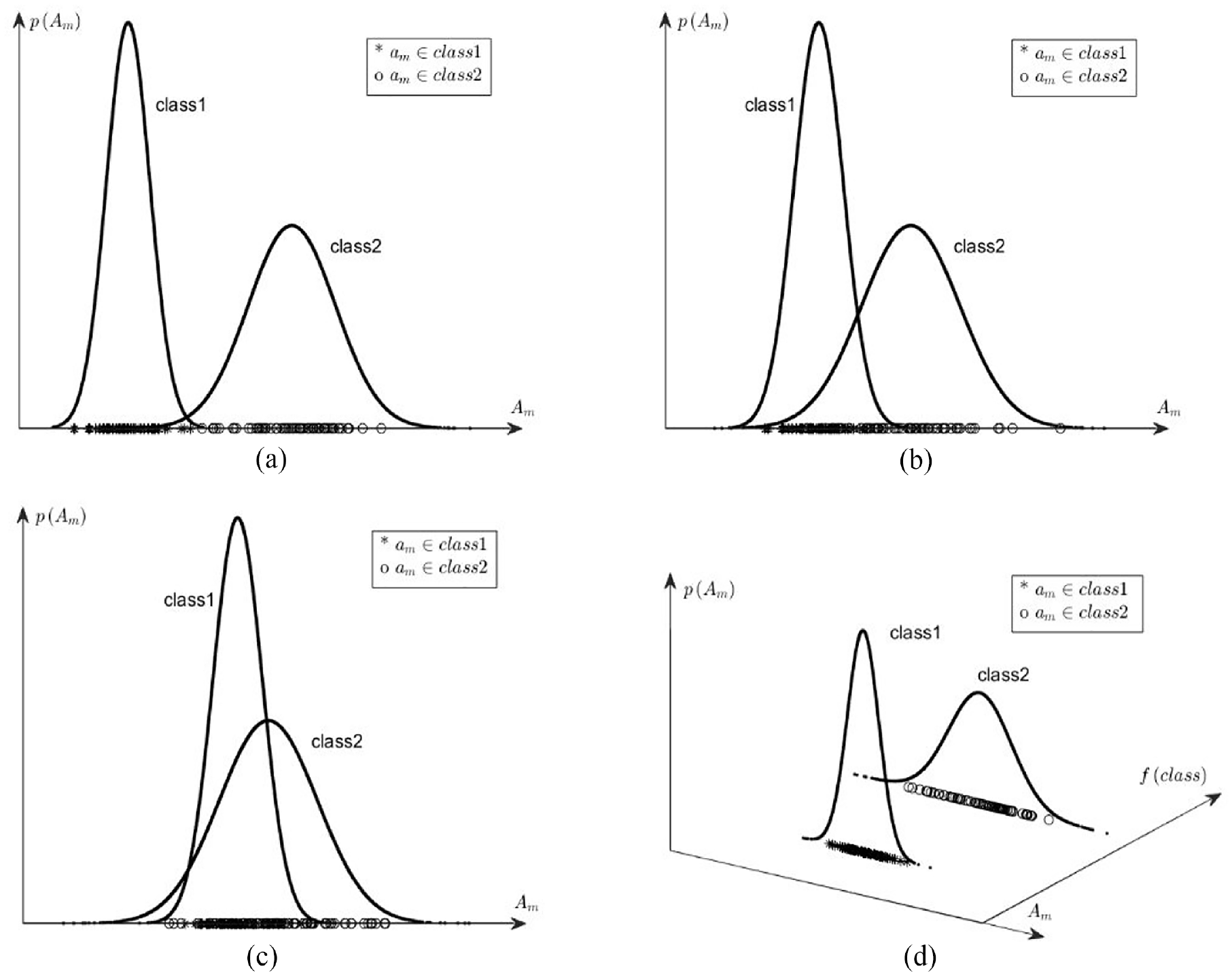
(a) Strong two-region distribution of
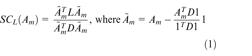
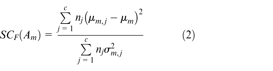
FS selects attributes with close intra-class values and scattered inter-class values. It scores the mth attribute
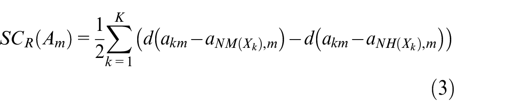
The relief scores the mth attribute
There is no trace of sample class labels in the above expressions. In fact, the implicit mapping between the distribution of
In addition, when the implicit single mapping between the distribution of
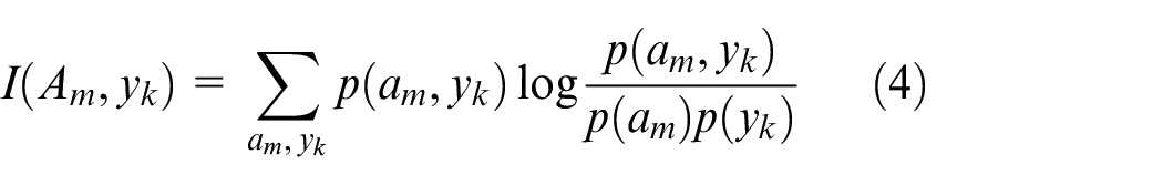
MIFS makes use of class labels in an explicit way, and it focuses on mutual information to evaluate the relevance of attributes and classes, and attributes to attributes, but it underexpresses the sample property of “intra-class to tight, inter-class to sparse.” In summary, this paper investigates a way to explicitly fuse class labels with attributes, and organizes the fused data in a clustering manner to discriminate the class differentiation ability of attributes based on inter-cluster and intra-cluster distances, and proposes a feature selection algorithm based on class labels, SOM, and hierarchical clustering.
Feature selection for binary classification based on class labeling and clustering
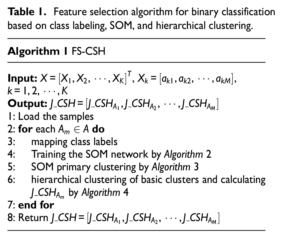
The proposed algorithm is shown in Table 1, which evaluates all the attributes one by one. Because of the need to explicitly use the guidance role of the class labels, this algorithm firstly fuses the sample values with their class labels to generate new 2-D vector samples. Then considering that attributes with significant classification performance possess the characteristics of similar (or close) attribute values for samples of the same class and large (or far) differences in attribute values for samples of different classes, this algorithm uses SOM neural network clustering and hierarchical clustering to automatically organize the division of the two-dimensional vector samples; Finally, the evaluation function of attribute
Feature selection algorithm for binary classification based on class labeling, SOM, and hierarchical clustering.
Mapping class labels
In order to play a guiding role of class labels in the feature selection process, the attribute values of the samples are combined with the class labels. For the attribute
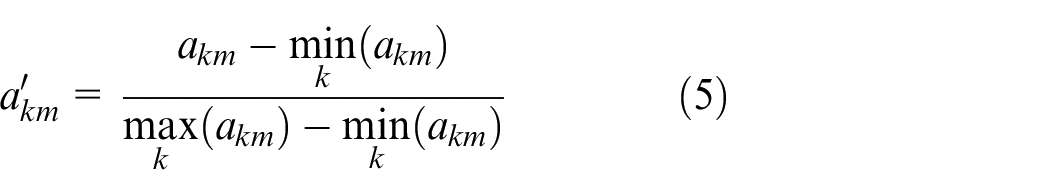
Using equation (5) to normalize all the sample values of
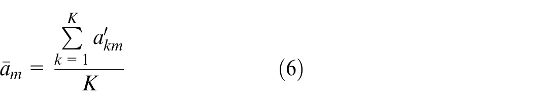
Equation (6) gives the normalized sample mean

Equation (7) maps the class label
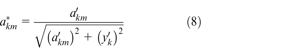
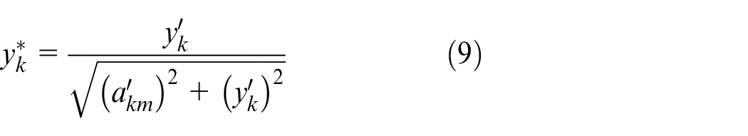
Through the above steps, the two-dimensional vector
Training the SOM network
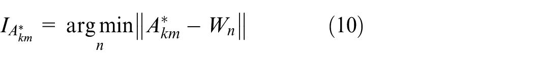
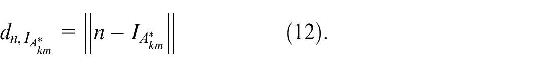
SOM neural network is different from other neural networks and also different from other clustering algorithms. It is able to reproduce the topological relationships among the input patterns with the topological relationships of the output layer neurons obtained from the mapping, and the spatial distribution of the trained network connection weight vectors reflects the statistical properties of the input patterns. 26 The general SOM neural network adopts a “planar” topology, which maps the high-dimensional input patterns to the output layer neurons with two-dimensional planar distribution through competition, cooperation, and adaptive steps, and reflects the aggregation characteristics of the input patterns by the distribution characteristics of the weight vectors of these neurons to form clusters after clustering. 27 At this case the clusters are distributed on a two-dimensional plane, which can complicate the subsequent hierarchical clustering. In fact, as mentioned in the literature, one-dimensional SOM is significantly superior than two-dimensional SOM in many aspects such as maintaining and achieving linear separability of classes, expressing the similarity between data and the clarity of inter-class location relationships, and the ease of visualizing class boundaries. 28 In addition, using clustering methods based on one-dimensional SOM to cluster unknown datasets can overcome the problem of not knowing the structure of the dataset and not being able to choose the correct clustering method, avoid the phenomenon of not getting the correct clustering results due to the unsuitability of the method, and provide a method to ensure that the clustering and structural characteristics of the unknown dataset can be better discovered. 28 The one-dimensional SOM can be used as the basis for clustering any type of dataset. Therefore, in this paper, a one-dimensional SOM is chosen and the output layer neurons are organized in a ring topology, as shown in Figure 2. It has l source nodes in the input layer and n neurons in the output layer, with full connectivity between neurons and source nodes. The neurons in the output layer are topologized in the form of a “closed curve,” where any neuron is directly connected to the neurons on either side of it, and the inhibition of the winning neuron on its neighboring neurons extends along both sides of the curve during the “weight coefficient update” phase of network training. The Gaussian topology field of winning neuron is shown in Figure 3. The neurons in the output layer after SOM training are distributed along the closed curve.
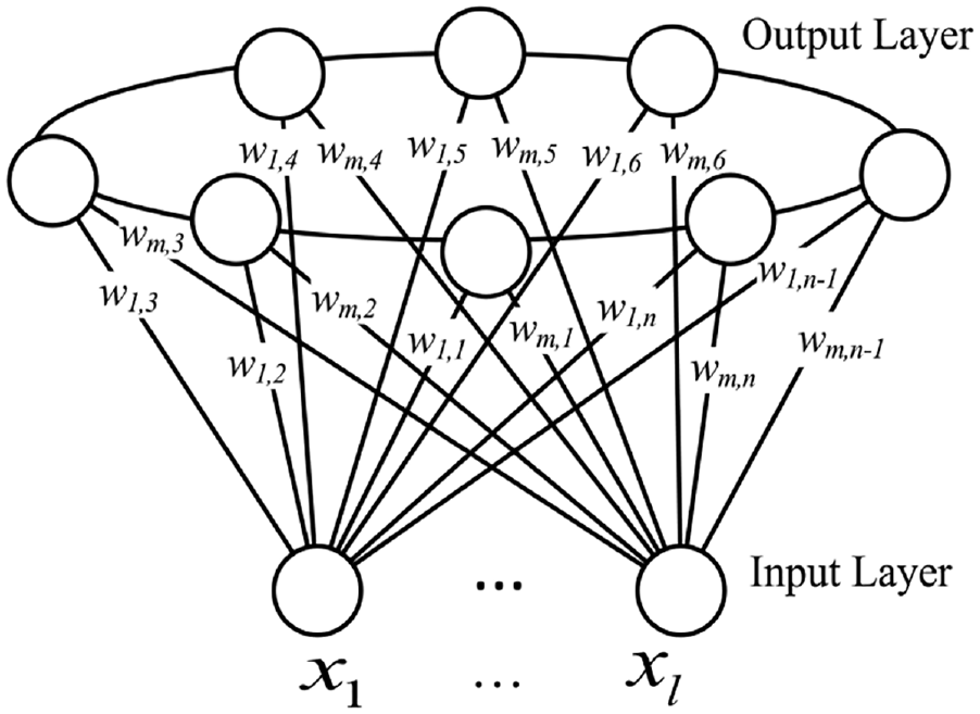
One dimensional ring SOM structure.
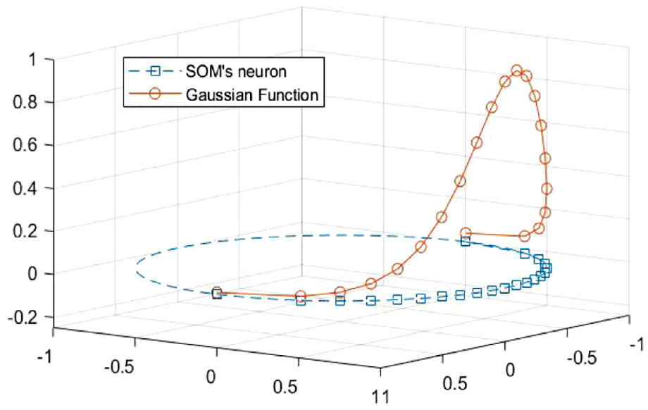
Gaussian topology field of winning neuron.
Training SOM network.
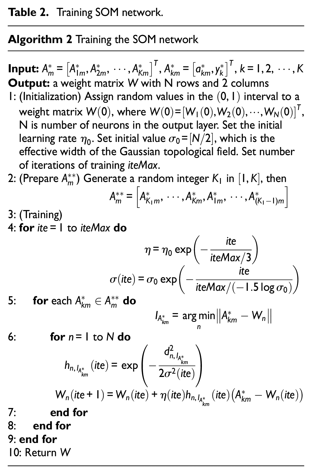
The winning neuron during the competition for SOM training is noted as
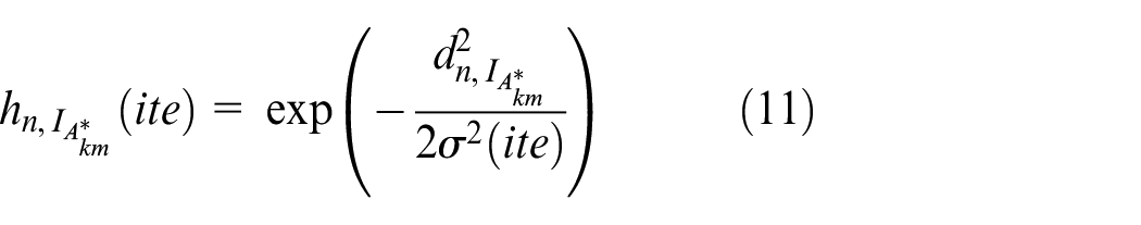
Where
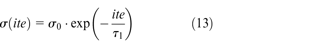
To accelerate the rate of Gaussian topological field reduction, the constant

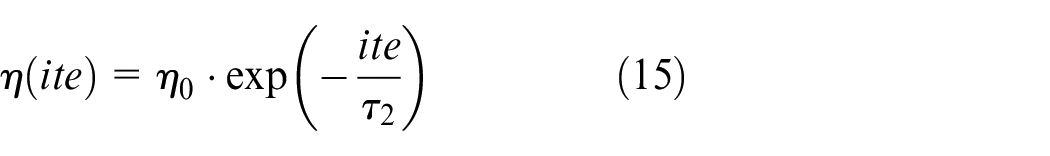
To ensure the convergence accuracy of SOM training, the constant

At the end of the network training, the neurons in the output layer are mapped and shot to different locations in the ring topology, which was influenced by the two-dimensional vector
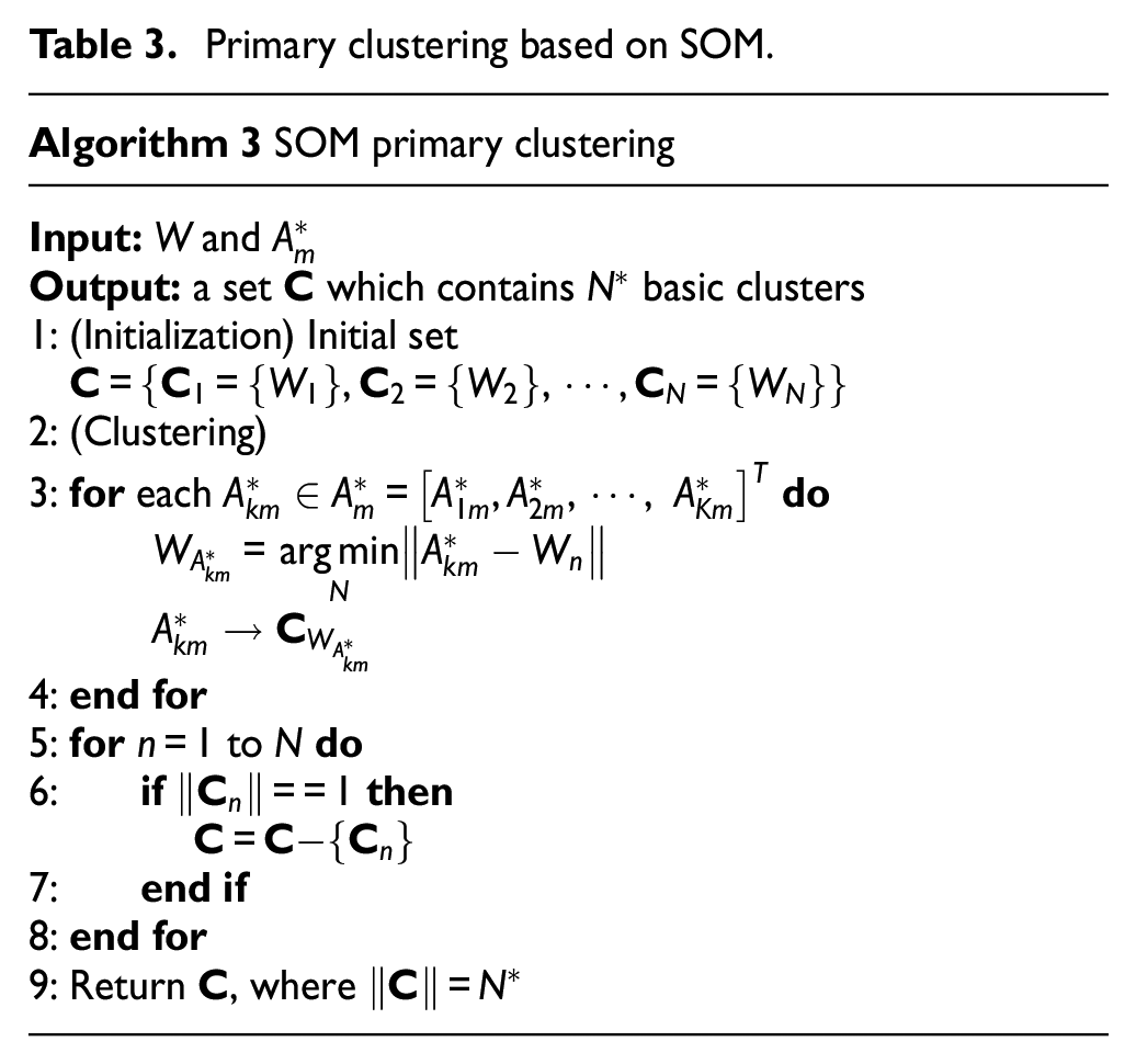
SOM primary clustering
In order to achieve binary clustering of the two-dimensional vectors
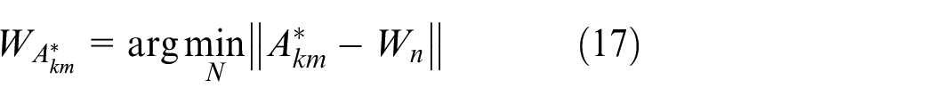
Primary clustering based on SOM.
Cohesive hierarchical clustering of basic clusters
On the basis of the primary clustering, cohesive hierarchical clustering is performed on the basic clusters until only two clusters remain. At this point all two-dimensional vectors
Cohesive hierarchical clustering of basic clusters.
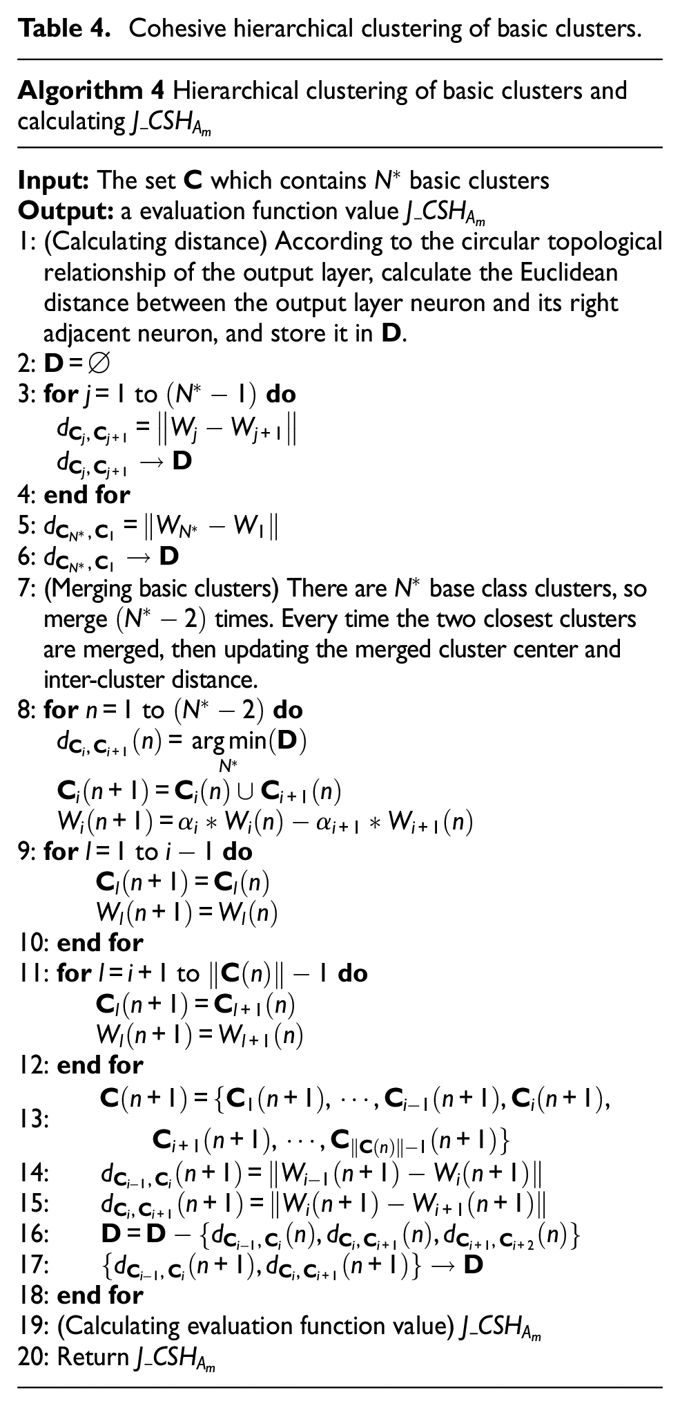
In the hierarchical clustering, the Euclidean distance between the neuron in the output layer and its right neighboring neurons is calculated in turn with reference to the “circular” topology of the SOM output layer and stored in the distance set

Where
Collate the set
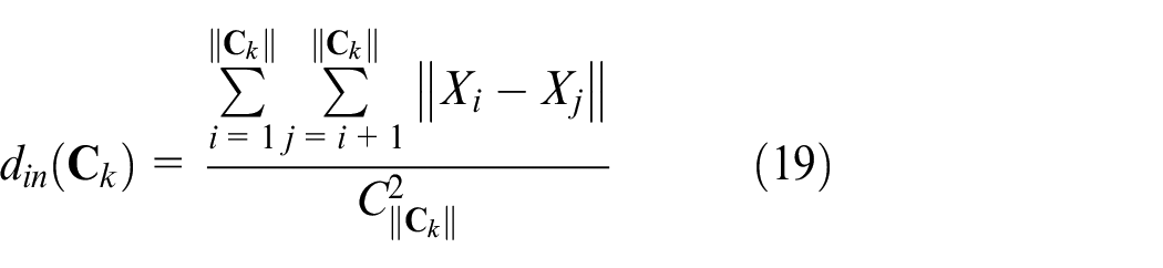
Where

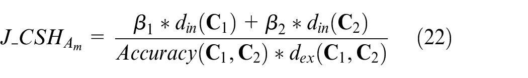
Where
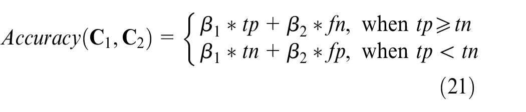
Where
Time complexity analysis of the algorithm
In terms of time complexity, firstly, the number of attributes M affects the time overhead of the above algorithm as it calculates the evaluation function for all attributes one by one. Secondly, the training process of the SOM network takes up most of the time compared to the initial and hierarchical clustering process when examining any of the attributes, and the time overhead of the process is mainly determined by the number of iterations
Experimental analysis and discussion
Software resources used for the experiments include: Python 3.8.11 (https://www.python.org/) and Spyder IDE 5.1.5 (https://www.spyder-ide.org/). They are used to provide a scripting language environment and an integrated development environment, respectively. The hardware platform of the computer used for the experiments is mainly: Intel Core i7-10750H 2.60 GHz processor and 8 GB 2933 MHz memory.
In order to test the algorithm proposed in this paper, firstly, artificial data are used to verify its ability and robustness in distinguishing attributes; secondly, for real data from different sources, the algorithm of this paper is used to compare with classical mainstream algorithms (such as MI,
20
FS,
9
LS,
10
and reliefF
12
) for feature selection and compare the performance of classifiers after feature selection by LR (Logistic Regression), K-NN (K-Nearest Neighbor), DT (Decision Tree), and SVM (Support Vector Machine) classifiers to evaluate the practicality of the FS-CSH algorithm. Regarding LR, the regularization parameters adopts “l2,” the optimization method of loss function is “liblinear,” the residual convergence condition is specified as
The relevant parameters of the SOM network in the experiments are set as follows: number of input units
Artificial data sets
Two-dimensional uniformly distributed data
Consider the classification problem in the two-dimensional feature space of Figure 4.20,29 The attribute vector of the sample
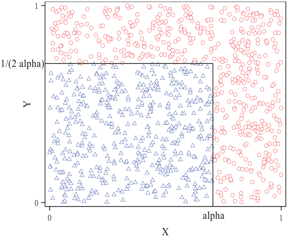
Two-dimensional sample distribution.
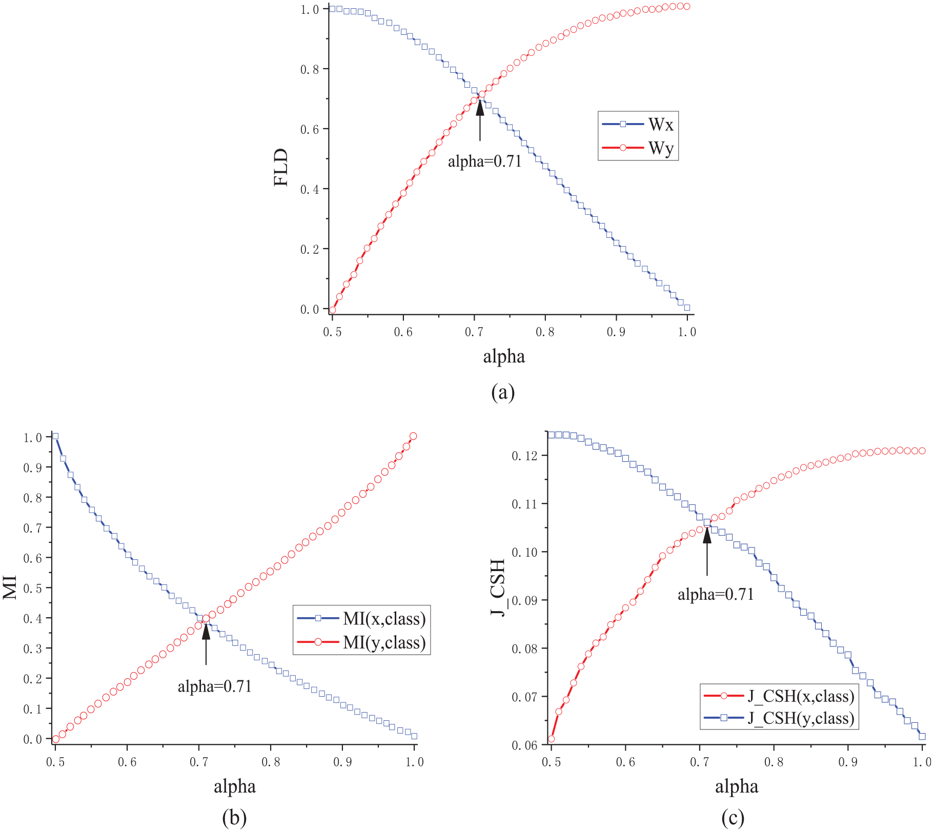
(a) Fisher linear discriminant vector values, (b) mutual information values, and (c) evaluation function values J_CSH.
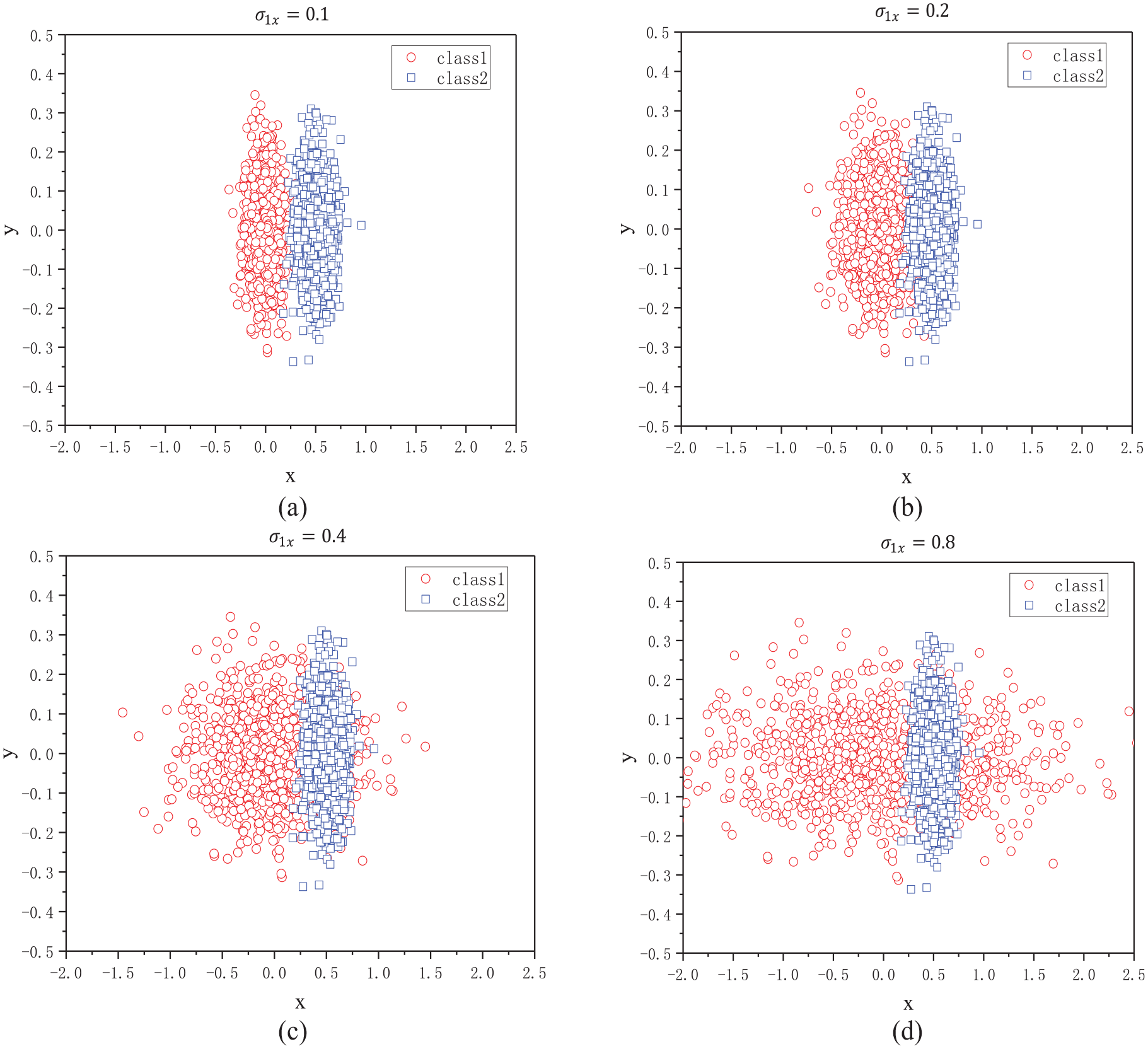
Two-dimensional Gaussian mixed probability density data
The robustness of the algorithm was verified by choosing different Gaussian probability densities for the case of binary classification of two-dimensional Gaussian mixed distribution data.
20
Consider a two-dimensional sample space attributed to two classes, with samples described by the attribute vector
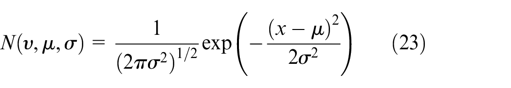
The Gaussian mixture probability density of class 1 and class 2 is simply expressed as:


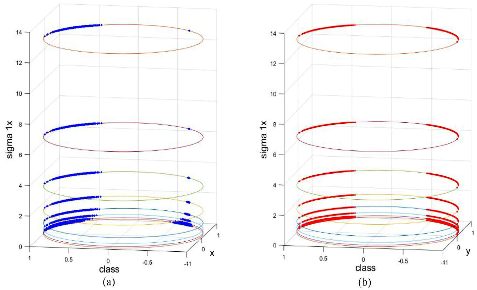
To simulate a real classification task, a series of value-added tests of
(a)
The attribute evaluation function values
Comparison of J_CSH, MI and FLD.
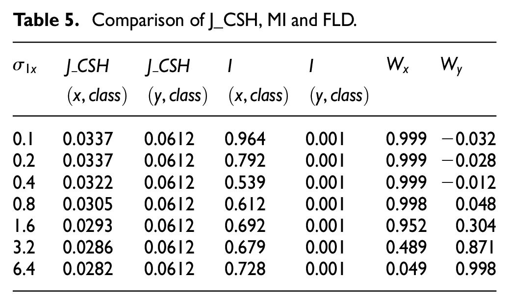
(a)
Real data sets
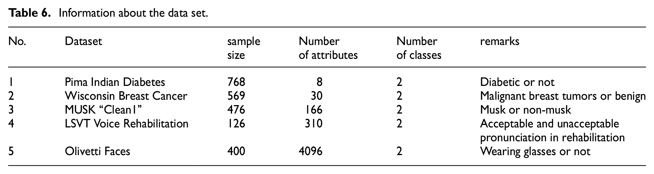
In the experiments, five binary classification datasets widely used for feature selection algorithms and classifier performance validation will be used, which belong to different domains and have a progressively increasing number of attributes and can be found in UCI (http://archive.ics.uci.edu/ml/index.php). These datasets include: Pima Indian Diabetes, Wisconsin Breast Cancer Database, 30 MUSK “Clean1” Database, 31 LSVT Voice Rehabilitation Dataset, 32 Olivetti Faces Database, as detailed in Table 6.
Information about the data set.
The feature selection algorithms of the same type: MIFS, FS, LS, and reliefF were selected for comparison. MIFS, FS, and reliefF are the higher scoring attributes are more important, and their scores are normalized to min-max; the algorithms in this paper and LS are the lower scoring attributes are more important, and their scores are normalized to min-max after taking the inverse. To evaluate the classification accuracy of the classifier after feature selection, 80% of the data are training data and 20% are test data, and the training data are subjected to 10-fold cross-validation for 20 times to test the classification accuracy; the test data are subjected to 20 classification experiments to obtain the classification accuracy.
Pima Indian Diabetes dataset
Pima Indian Diabetes was used to study the classification problem between the class label “diabetic or not” and eight attributes. It has 768 data of Pima Indian female patients over 21 years of age, 268 of them have diabetes and 500 do not. The proposed algorithm was used to calculate the J_CSH values of the eight attributes shown in Figure 8. The J_CSH values of these attributes, in descending order, were: 2 Glucose, 6 BMI, 3 Blood Pressure, 7 Diabetes Pedigree Function, 8 Age, 1 Pregnancies, 4 Skin Thickness, and 5 Insulin. The top-ranked attributes with J_CSH values were selected as the result of feature selection. The two attributes with the lowest J_CSH values were 2 Glucose and 6 BMI, which is consistent with the conclusion stated by the authors Chen et al., 33 and in line with the opinion of the authors Gong et al. 34 that the most dominant attributes in Pima India Diabetes are Glucose and BMI.
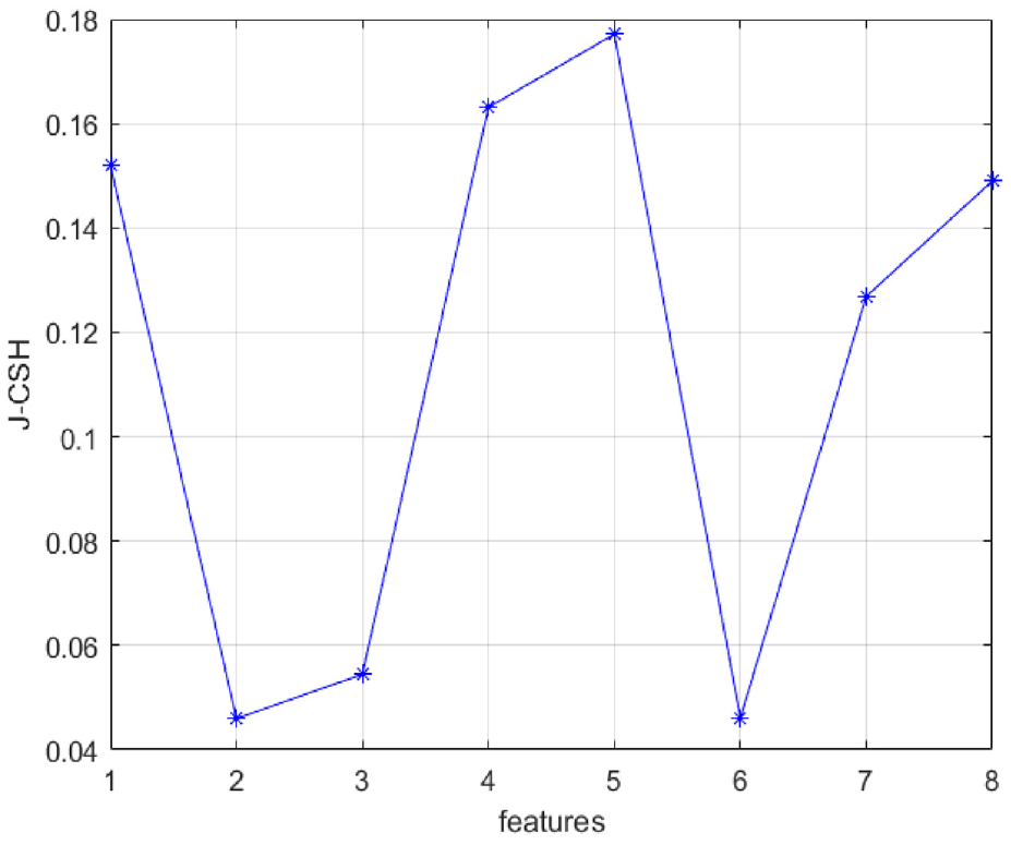
J-CSH value of features for Pima.
The scores of MIFS, FS, LS, relief, and the algorithm in this paper regarding all attributes are shown in Figure 9. MIFS and FS can select the attributes Glucose and BMI that have a major impact on the classification, while reliefF and LS undergo a deviation. The algorithm in this paper, FS_CSH, is not only able to select the important attributes that are effective for classification, but also its ability to point out the categories for attribute differentiation is more obvious.
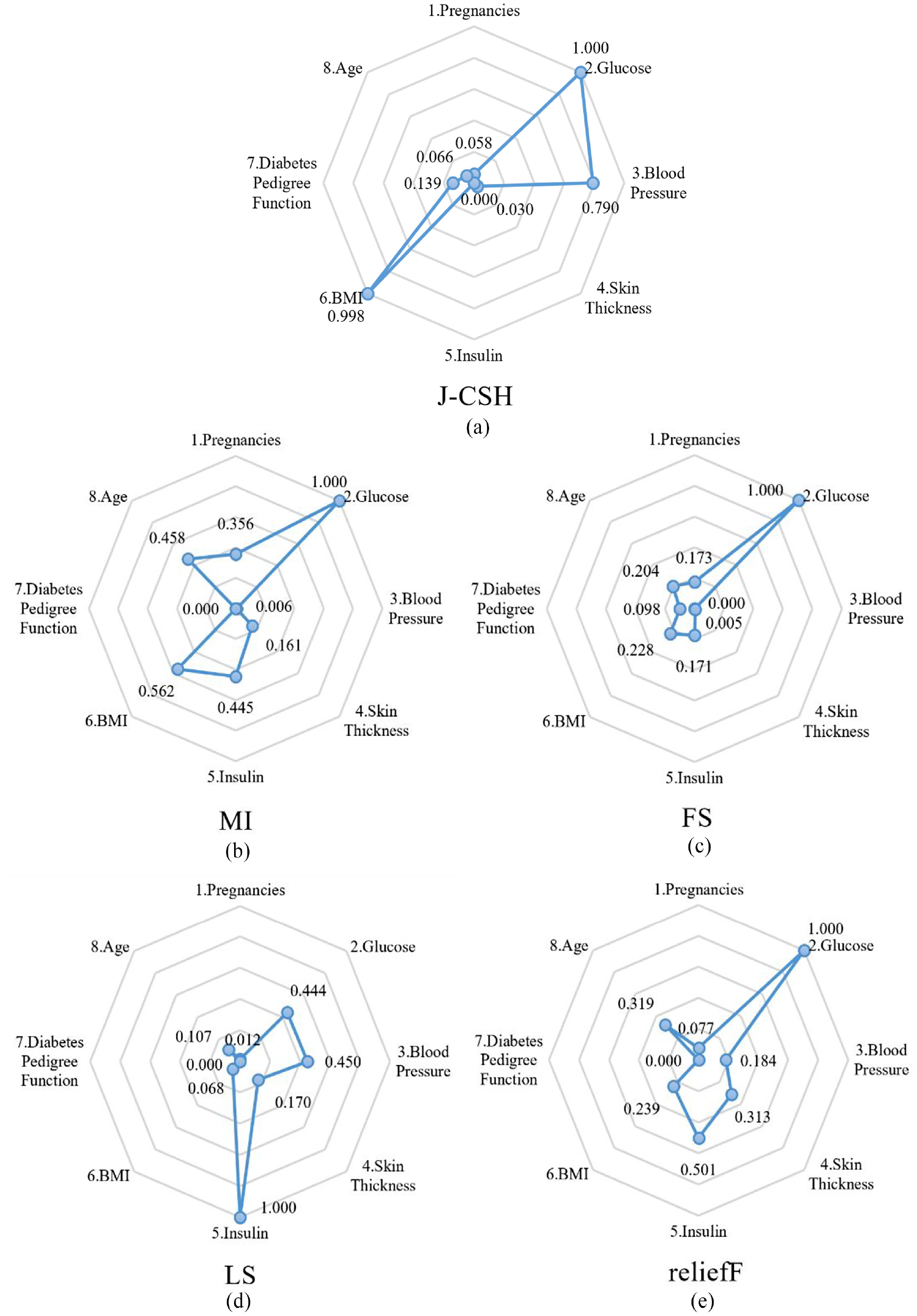
(a) J-CSH value of features for Pima, (b) MI value of features for Pima, (c) FS value of features for Pima, (d) LS value of features for Pima, and (e) reliefF value of features for Pima.
Finally, the impact of the above algorithms on the classification accuracy was evaluated using LR and SVM classifiers. The average value of accuracy after 20 times of cross-validation of 10 folds of training data is shown in Figure 10; the average value of accuracy after 20 times of classification of test data is shown in Figure 11. The attributes selected by the algorithm FS_CSH in this paper can effectively improve the classification accuracy, and its ranking of attributes is generally higher than the cases of other feature selection algorithms when different numbers of attributes are required.
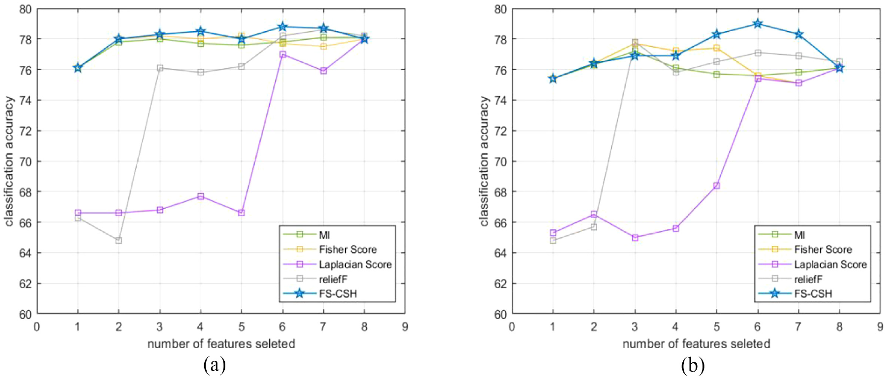
(a) LR_80%Train_10fold and (b) SVM_80%Train_10fold.
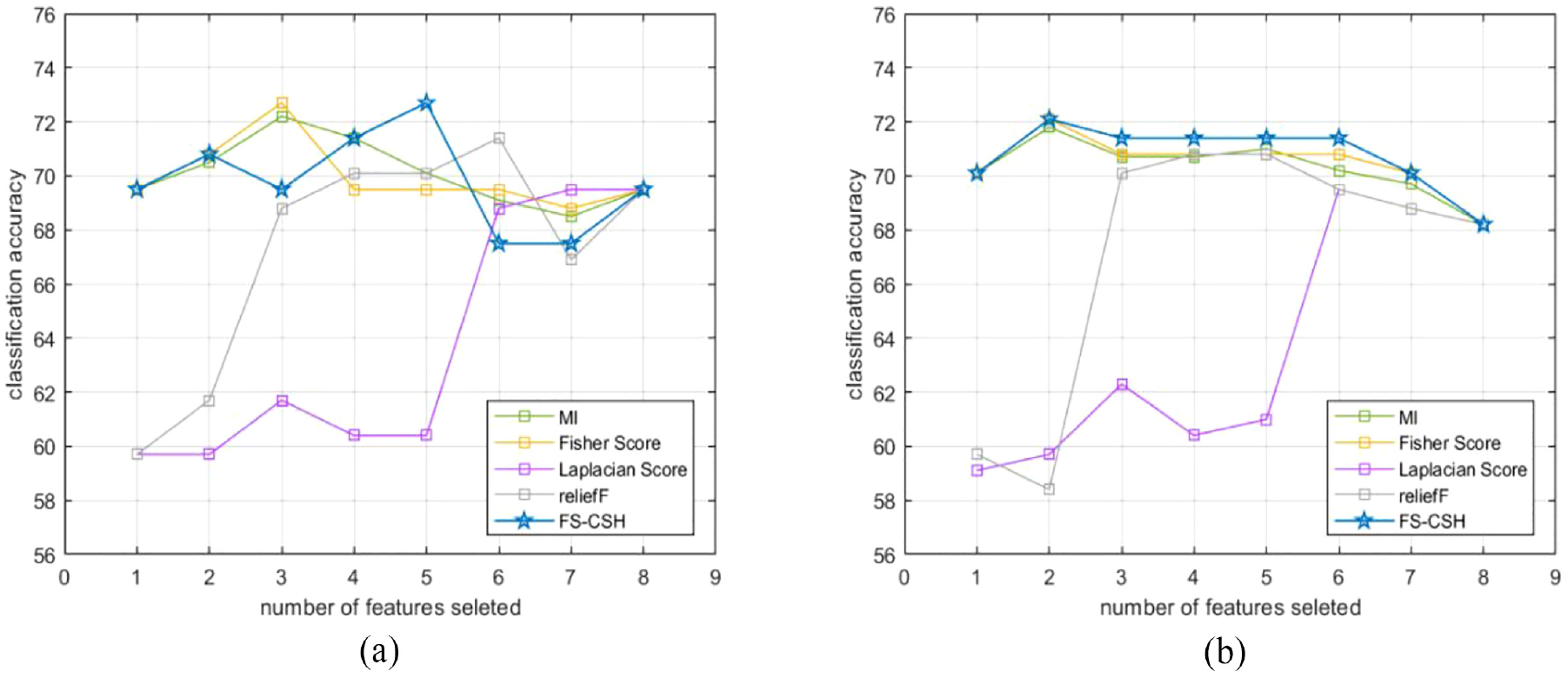
(a) LR_20%Test and (b) SVM_20%Test.
Wisconsin Breast Cancer dataset
The Wisconsin Breast Cancer dataset (WBCD) is pathological information of women with breast cancer in Wisconsin, USA. It contains data from 569 individuals, 212 of whom have malignant breast tumors and 357 of whom are benign, with 30 attributes per data entry. The evaluation function value J_CSH of the 30 attributes was calculated using the algorithm in this paper, as shown in Figure 12. The top 20% of J_CSH values in ascending order were selected: the 21st, 5th, 23rd, 1st, 3rd, and 28th attributes constituted a new feature subset. The classification accuracy of LR and SVM is verified by compared to the feature subsets selected by MIFS, FS, LS, and reliefF algorithms.
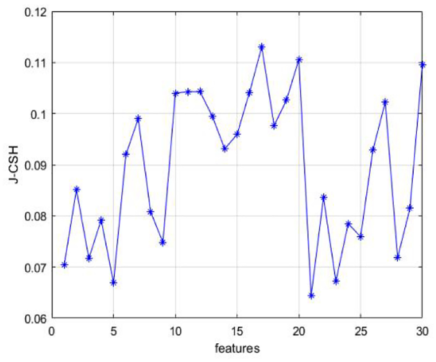
J-CSH value of features for WBCD.
Figure 13(a) shows the accuracy of 10-fold cross-validation for LR 80% training data, the proposed algorithm outperforms MIFS, relief, and FS algorithms overall, and is very close to the effect of LS algorithm. Figure 14(a) shows the accuracy of LR 20% test data, only in the case of attribute number 2 FS-CSH algorithm corresponds to 92.1% accuracy, which is slightly lower than MIFS, FS, and LS algorithms, but still higher than reliefF algorithm. The accuracy of the FS-CSH algorithm is either second or tied for first place with other algorithms for the number of attributes 1, 3, 4, 5, and 6.
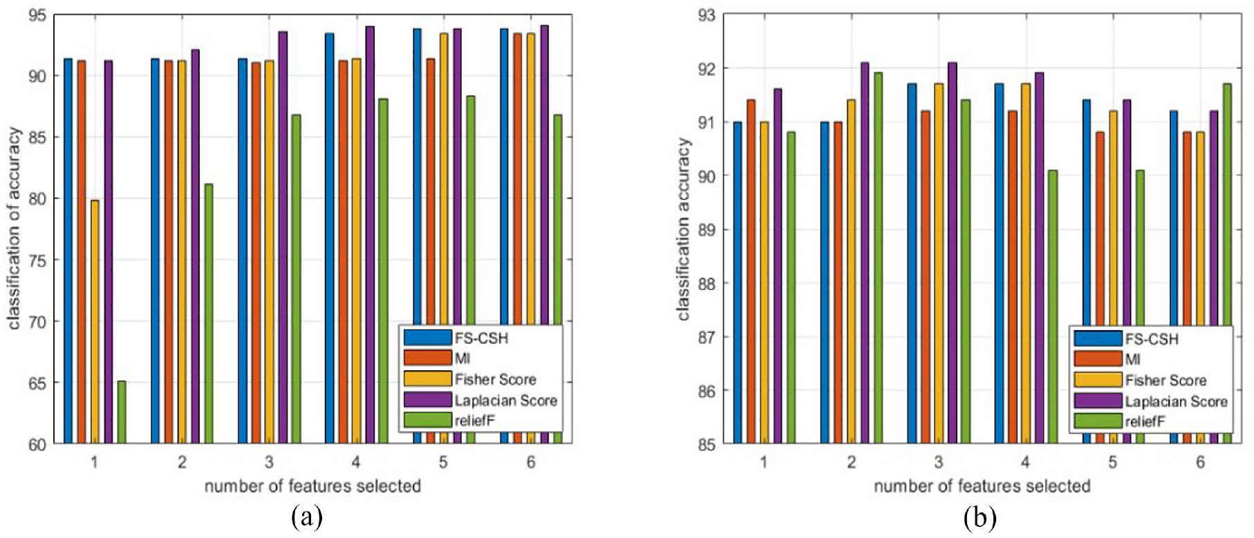
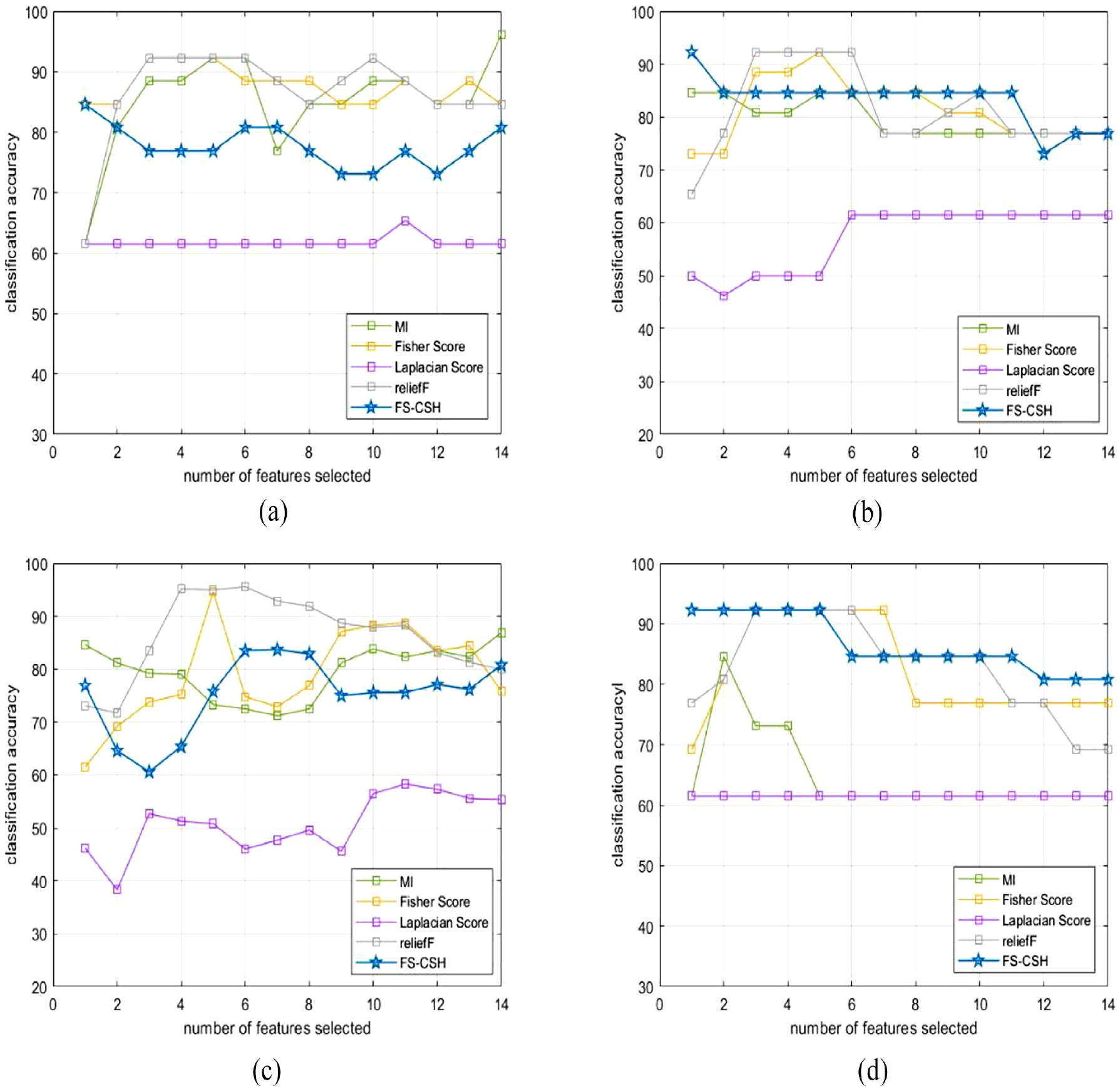
(a) LR_80%Train_10fold and (b) SVM_80%Train_10fold.
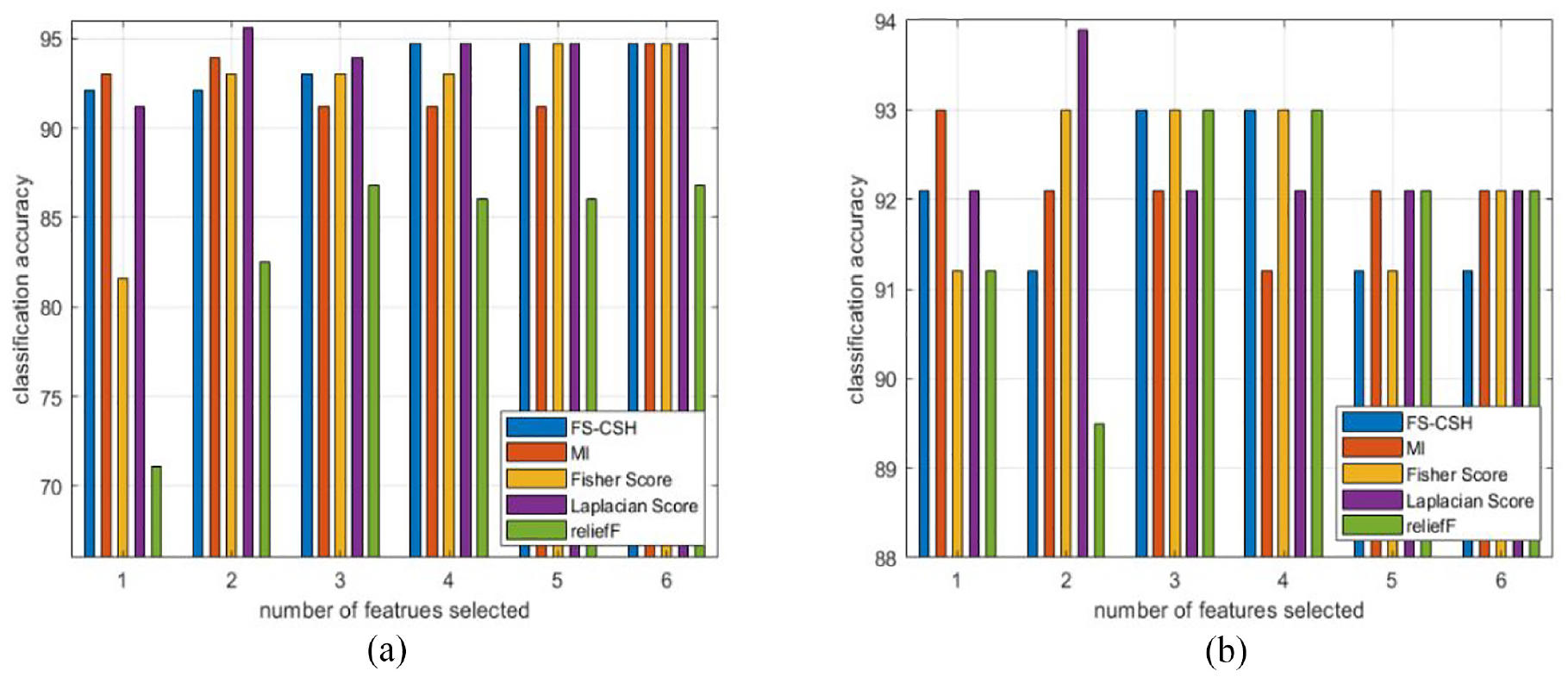
(a) LR_20%Test and (b) SVM_20%Test.
Figure 13(b) shows the classification accuracy of SVM 80% training data with 10-fold cross-validation. When the number of attributes is 1, the accuracy of the proposed algorithm is the same as FS, higher than reliefF, and slightly lower than MIFS and LS; when the number of attributes is 2, the accuracy of FS-CSH is the same as MIFS; when the number of attributes is 3 and 4, the accuracy of FS-CSH is the same as FS and only lower than that of LS; when the number of attributes is 5, the accuracy of FS-CSH is the highest; when the number of attributes is 6, the accuracy of FS- CSH has the same accuracy as LS and is only lower than the accuracy of the reliefF algorithm. Figure 14(b) shows the accuracy of SVM 20% test data. When the number of attributes is 1, the accuracy of FS-CSH is the same as LS, higher than FS and reliefF, and slightly lower than MIFS; when the number of attributes is 2, the accuracy of FS-CSH is slightly lower than MIFS, FS, and LS, but still stronger than reliefF; when the number of attributes is 3 and 4, the accuracy of FS-CSH is the same as FS and reliefF, and the highest; when the number of attributes is 5 and 6, the accuracy of The accuracy rate of FS-CSH still reaches 91.2%. The above analysis shows that the proposed algorithm is effective in the Wisconsin Breast Cancer dataset and can filter out the subset of features that are beneficial for classification.
MUSK “Clean1” dataset
The Clean1 part of the MUSK dataset contains 476 molecular samples, described by 166 attributes, 207 samples are labeled as “musk” and 269 as “non-musk.” The algorithm of this paper is used to calculate the evaluation function values of 166 attributes J_CSH, as shown in Figure 15. Considering that the MUSK dataset is the structural description of microscopic molecules with linear indistinguishability, the classification accuracy of the above-mentioned feature subsets is examined on K-NN, DT, and SVM, as shown in Table 7. The accuracy of the proposed algorithm is lower than MIFS and reliefF only when the 10-fold cross-validation of 80% training data is performed on DT, and the remaining cases are higher than other algorithms. It can be concluded that the proposed algorithm FS-CSH is effective on the MUSK “Clean1” set, and the algorithm can filter the subset of features favorable for classification when the number of attributes is 10% of the total.
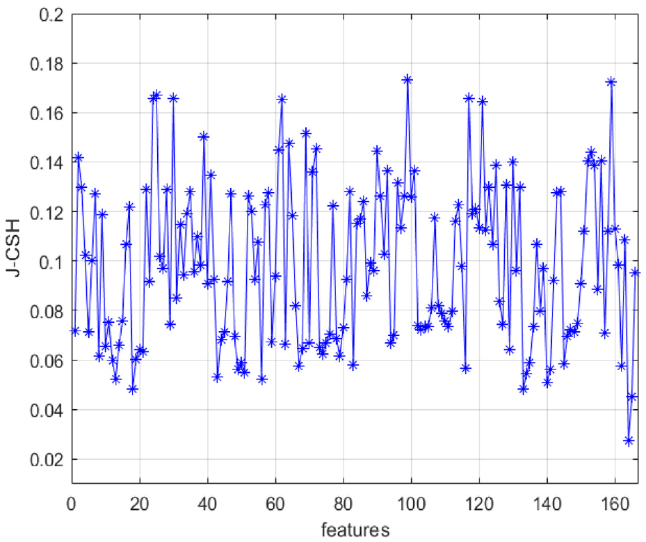
J-CSH value of features for MUSK.
Average classification accuracy of K-NN, DT, and SVM.
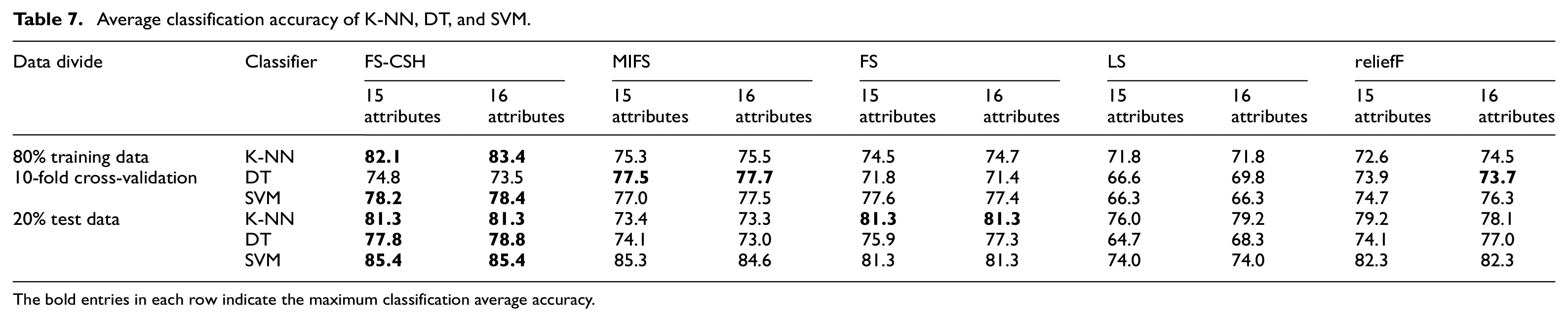
The bold entries in each row indicate the maximum classification average accuracy.
LSVT Voice Rehabilitation dataset
LSVT Voice Rehabilitation was created by Athanasios Tsanas of the University of Oxford, who obtained clinical information on 14 patients from the voice signals provided by LSVT Global. These patients were diagnosed with Parkinson’s disease and were receiving LSVT-assisted voice rehabilitation. The set characterizes 126 speech signals using 309 algorithms, that is, it has 126 samples of speech signals, each described by 309 attributes and labeled as “acceptable” and “unacceptable.”
Due to the specificity of the data distribution of each attribute in this dataset, it is more challenging to perform operations such as feature selection, feature extraction, and classifier performance validation on this dataset. In this experiment, a two-step preprocessing was performed on this set: 1 Eliminate attributes with small variances. The unbiased estimated variance of
The evaluation function values J_CSH of the remaining attributes were calculated using the algorithm in this paper, and the values of J_CSH for the excluded attributes were set to 0.2 uniformly, as shown in Figure 16. The two attributes with the lowest J_CSH values were: 153 entropy_log_4_coef and 84 MFCC_0th coef. On LR, K-NN, DT, and SVM, compared with algorithms such as MIFS, FS, LS, and reliefF are shown in Figures 17 and 18.
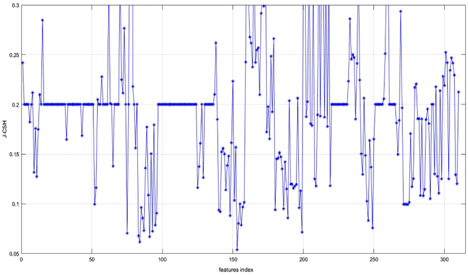
J-CSH value of features for LSVT Voice Rehabilitation dataset.
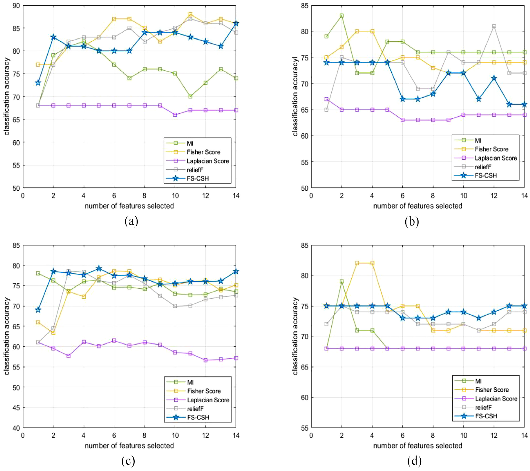
(a) LR_80%Train_10fold, (b) K-NN_80%Train_10fold, (c) DT_80%Train_10fold, and (d) SVM_80%Train_10fold.
(a) LR_20%Test, (b) K-NN_20%Test, (c) DT_20%Test, and (d) SVM_20%Test.
Figure 17 shows the accuracy of the 10-fold cross-validation for 80% of the training data for the four classifiers. With the number of attributes of 2, the accuracy of the proposed algorithm is highest on LR and DT, inferior to MIFS, FS, and reliefF on K-NN, and equal to FS and reliefF and slightly inferior to MIFS on SVM. When the number of attributes is greater than 2, the accuracy of the proposed algorithm is comparable to other algorithms, only inferior to MIFS, FS, and reliefF on K-NN.
Figure 18 shows the accuracy of 20% of the test data for the four classifiers. With the number of attributes of 1, the accuracy of the proposed algorithm is only slightly lower than the MIFS algorithm on DT, and higher or equal to the rest of the algorithms. For the number of attributes >2, the proposed algorithm shows higher accuracy with MIFS, FS and reliefF on K-NN and SVM, better than LS on LR, and indistinguishable from MIFS, FS, and reliefF on DT. In summary, for the high-dimensional complex dataset LSVT Voice Rehabilitation, the algorithm FS-CSH still shows a trustworthy screening ability and its selected feature subset is effective in improving the classification accuracy of the classifier.
Olivetti Faces dataset
The Olivetti Faces set contains a total of 400 face images from 40 subjects with 10 faces each. Each image is 64 × 64 pixels, described as a 4096-dimensional vector, and each pixel has 256 gray levels. For this set, determining whether a person is wearing glasses or not is a typical binary classification problem. Before the experiment, this face image data was histogram equalized, and each piece of data was assigned a label of 0 or 1 depending on whether the face in each image was wearing glasses, with 1 being wearing glasses and 0 being not.
The 4096 attribute (pixel) evaluation function values J_CSH are calculated using the algorithms in this paper, as shown in Figure 19. Then the scores of MIFS, FS, LS, and reliefF algorithms are calculated for each attribute (pixel). The top 32 to 256 attributes (pixels) of each algorithm are selected to construct new feature subsets, and the classification accuracy of the selected feature subsets is checked by SVM.
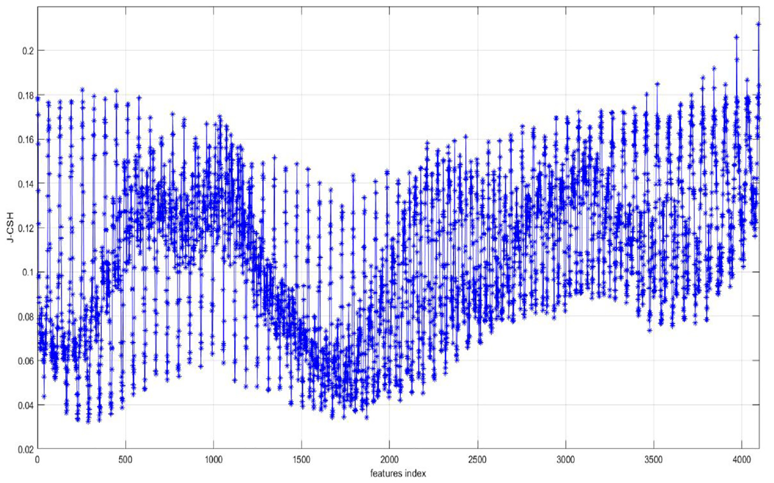
J-CSH value of features for Olivetti Faces.
In Figure 20(a), the average accuracy of the proposed algorithm is slightly lower than the MIFS algorithm when the number of attributes (pixels) is 32 and 64, on par with FS and reliefF, and higher than the LS algorithm; in the rest of cases, the average accuracy algorithm proposed in this paper is comparable to that of MIFS, and higher than other similar algorithms. In Figure 20(b), when the number of attributes (pixels) grows from 32 to 296, the average accuracy rates of FS-CSH, MIFS and reliefF alternately lead: FS-CSH leads four times, MIFS algorithm leads one time and reliefF algorithm leads three times. And they all have higher average accuracy than the FS and LS algorithms.
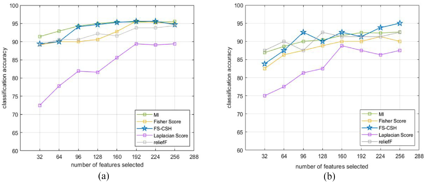
(a) SVM_80%Train_10fold and (b) SVM_20%Test.
To visualize the effect of the proposed algorithm on the selection of face pixels, Figure 21(a) shows 119 images of faces wearing glasses out of 400 face data, and Figure 21(b) shows the distribution of selected pixels (marked by black pixel dots) in these face data images. Comparing Figure 21(a) and (b), the pixel points selected by the proposed algorithm are mainly concentrated in the cheek area below the eyes, while avoiding the frame area. The former is influenced by the refractive effect of the eyeglass lens, which makes this part more favorable for distinguishing whether glasses are worn or not; while the latter is influenced by the lateral shadow of the eyebrows and the bridge of the nose, resulting in its ineffectiveness for determining whether glasses are worn or not. Therefore, it can be concluded that the feature selection algorithm FS-CSH proposed in this paper is effective on the set of Olivetti Faces and can filter out the subset of features that are favorable for classification, which is slightly superior to the MIFS and reliefF algorithms that also utilize classification information.
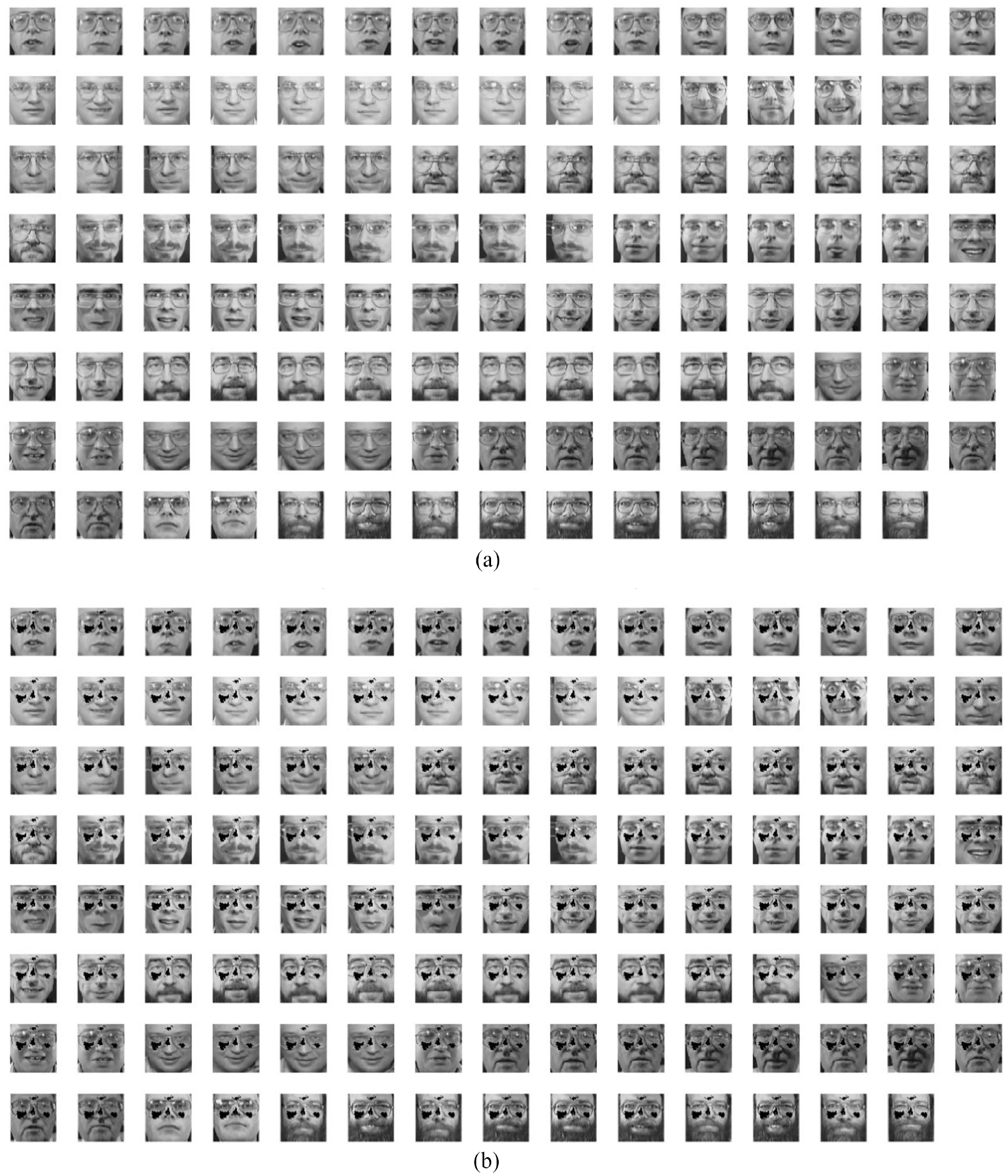
(a) Pictures of people wearing glasses and (b) selected pixels on pictures of people wearing glasses.
Conclusion
In this paper, a feature selection algorithm FS-CSH is proposed for the binary classification problem. The algorithm explicitly incorporates class labels, goes through SOM and hierarchical clustering, scores each attribute, evaluates their relevance to the category, and filters the subset of features with the maximum decision classification capability that can improve the classification accuracy of the reduced-dimensional dataset. The results of simulation applications on both artificial and real data show the above results. Compared with feature selection algorithms of the same type (i.e., algorithms that examine each attribute for scoring), the one proposed in this paper is a heuristic algorithm with a clear physical meaning, simple computation, effective, and robustness.
Footnotes
Acknowledgements
We gratefully thank the Action Editor and anonymous reviewers for their constructive comments.
Declaration of conflicting interests
The author(s) declared no potential conflicts of interest with respect to the research, authorship, and/or publication of this article.
Funding
The author(s) disclosed receipt of the following financial support for the research, authorship, and/or publication of this article: This work was supported by National Key R&D Program of China (2018YFB1703105) and National Natural Science Foundation of China (grant no. 51865027).