Sage Journals: Discover world-class research

Abstract

In this study, we propose a novel controller architecture and design for the automatic control of agricultural mobile robots to be used in farms and greenhouses. There are two novelties of this study. The first novelty is a completely new type of controller architecture proposed in which reference inputs and measured outputs are fed separately independent from each other to the controller. The controller architecture currently used in the literature uses only the difference between reference and measurement which is the error signal. The proposed architecture in this study is completely novel in the sense that not only the error information is used in the controller but also the information in reference inputs and information in measured outputs are used separately. This means a completely new type of look to control system by utilizing the information maximally in order to achieve superior performance. This performance boost is shown in the paper where the proposed architecture achieves up to 2000% better performance compared with state-of-the-art controllers. Second, controller architecture is grown to a complex structure from an initially simple PID structure. Using the maximal information comes with the cost of computational complexity to design the controller. The second novelty of growing the controller from initially simple PID equivalent controller tackles this difficulty by making the problem tractable and efficient to compute. This way the proposed novel controller can be designed within minutes in a commercially available laptop computer. The proposed controller is tested on a simulated agricultural mobile robot and results are compared with a previous state-of-the-art optimal controller. It is believed that the proposed architecture will be dominant in future automatic controllers and make current state-of-the-art controllers obsolete. This is because of the full utilization of information in controller design which results in robust disturbance rejection performance.

Keywords

Agricultural mobile robot intelligent control single-layer neural-network

Introduction

The use of robotics in agriculture is increasing every day. Robots are mainly used for inspection, planting, harvesting, irrigating, and pest control among other tasks. Agricultural mobile robots help farmers increase their effectiveness and efficiency by automating tasks normally done by human beings. In order to accomplish these tasks automatically, an agricultural mobile robot must have a great degree of autonomy. Autonomous agricultural mobile robots must be able to adjust their linear and angular speed depending on the requirements of the current task they are accomplishing. A lot of work is done in the literature for mobile robot speed control.

A global overview of mobile robot strategies is reviewed and reported by Tzafestas.¹ Among several control strategies, fuzzy and neural control methods are emphasized as intelligent controllers. Adaptive sliding mode attitude control of the wheeled mobile robot is implemented by Pang et al.² Radial basis function neural networks are used for learning. An adaptive neural control strategy for a wheeled mobile robot is used by Eskander Dagher et al.³ In this study, online tuning evolutionary slice genetic algorithm is used for learning parameters of neural networks. In another study,⁴ a reinforcement learning-based optimal controller is used for controlling three mecanum-wheeled mobile robots. The Lyapunov-based analysis is done to probe the stability of the system. In a study by Canbek et al.,⁵ recurrent neural networks (RNN) are used to control a holonomic mobile robot. Positioning drift is estimated using an RNN-based drift compensation algorithm. In In Liu and Cong’s⁶ study, control of a wheeled mobile robot is done using neural networks. Internet of Things (IoT) sensors are used to measure the dynamics and necessary control actions are done using radial basis function networks. In Janglová’s⁷ study, both motion planning and intelligent control of the wheeled mobile robot are done using artificial neural networks. In this study, two layers of neural networks are used. Neural networks are used as closed-loop controllers for mobile robot motion control in the study of Velagic et al.⁸ The error signal is fed to the neural network controller similar to most general cases. In another study,⁹ both simulation and real robot experiments are conducted for tracking control of the wheeled mobile robot. Differential games and H_∞ control are applied as controllers and disturbance rejection capabilities are observed. Nonlinear trajectory tracking control of a nonholonomic car-like mobile robot is considered, reported in Yang et al’s¹⁰ study. Simulation results are displayed and reported using the dynamic feedback linearization technique utilized to ensure stability. In the study of DeVon and Bretl,¹¹ the problem of stabilizing a unicycle-type mobile robot using a time-invariant, discontinuous control law is considered. Simulation results are reported using invariant manifold theory to explain quadratic dynamics. State feedback control law is utilized to ensure the stability of a simple wheeled mobile robot and the performance of the system in presence of model errors and measurement noise is demonstrated in Astolfi’s¹² study. In the study of Tayebi et al.,¹³ the invariant manifold approach is used to show the stabilization of n-dimensional nonholonomic chained systems. A mobile robot is controlled to show the proposed approach’s performance. Tian et al.¹⁴ reported the simulation results of a time-invariant discontinuous feedback law developed to stabilize a wheeled mobile robot. Wheel slippage is also included to have a more realistic mathematical model. Simulation results are reported. In another study,¹⁵ tracking control of wheeled mobile robots with nonholonomic constraints is studied. Nonlinear brushless DC motors are used as actuators and results are reported. Ashoorirad et al.¹⁶ propose wheeled mobile robots, controlled using a model reference adaptive algorithm. Feedback linearization is used to enhance stability. In Rigatos et al.’s¹⁷ study, the reduced complexity sliding-mode fuzzy-logic control technique is used to control mobile robots. Simulation is done to prove the stability of the proposed approach. Tzafestas et al.¹⁸ suggest control of autonomous nonholonomic mobile robots done using a digital fuzzy logic controller. FPGA is used as a controller platform and experimental results are reported. In the study of Das and Kar,¹⁹ trajectory tracking control of nonholonomic mobile robots is done using an adaptive fuzzy controller. A fuzzy logic system is used for function approximation and the system stability is proved using the Lyapunov stability theory. Simulation and real robot experiments are conducted and results are reported.

Optimal control is not limited to mobile robot platforms but other platforms like quadcopters are also controlled using various optimal control techniques. In Altan’s²⁰ study, performances of two metaheuristic optimization algorithms are compared, namely PSO and Harris Hawks Optimization (HHO). Altitude and attitude control of quadcopter is performed using PID control technique and parameters of the PID controller are optimized using aforementioned optimization algorithms. It is shown that HHO’s performance is higher than that of PSO. In Altan et al.’s²¹ study, a hexacopter with load transporting system is controlled using Nonlinear AutoRegressive eXogenous (NARX) neural network model. The performance of the NARX based controller is shown to be better than that of PID based controller. In Slama et al.’s²² study, error and reference signals are used to calculate the control signal with a neural network structure. Both indirect adaptive controller and adaptive PID controller structures are utilized outputs of which are selected using a switch. Experiments with and without disturbance are conducted on nonlinear MIMO systems and results are reported. In another study of Slama et al.,²³ adaptive PID controller is used to control nonlinear MIMO systems. Parameters are tuned using neural networks.

Some recent studies on intelligent mobile robot control also exhibit encouraging results. In Mondal et al.’s²⁴ study, a twofold hybrid control law is proposed. The proposed controller combines the feedback linearization controller (FBC) with the fuzzy logic controller (FLC). Simulations are run for a differential driven wheeled mobile robot with some dynamic obstacles on the path and results are reported. In Thai et al.’s²⁵ study, differential driven wheeled mobile robot is controlled using variable parameter PID controller. The desired trajectory of the robot is generated using NURBS curve. Both simulation results and experimental results on real robot are reported. In Li et al.’s²⁶ study, a dual closed-loop trajectory tracking control strategy for a non-holonomic wheeled mobile robot (WMR) was developed. Sliding mode control was used for inner loop and a simple kinematic controller was used for outer loop. Experiments are conducted on real wheeled mobile robot and a comparison was done with PI controller.

In this study, linear and angular speed control of the agricultural mobile robot is done. A novel controller architecture is proposed and tested. One novelty of the proposed controller is in handling the input information. Classical controllers in the literature use only the error information from input. Some controllers also use reference signal along with the error signal. In the novel controller proposed in this study not only the current values of reference and measured output signals are used but short history of both signals and a short future history of reference input is used to calculate the control signal. This way much more information is utilized to calculate the control signal and as expected better performance is observed as reported in the results section. The organization of the paper is as follows: A brief introduction and literature survey are done in this first section. Materials and methods are given in the following section including the mathematical model of the agricultural mobile robot, the structure of the classical PID controller and proposed novel controller, and a brief explanation of the PSO algorithm. In the third section, results are given in figures. Discussion with remarks is provided in the fourth section. The conclusion and future work are written in the fifth section.

Materials and methods

Mathematical model of agricultural mobile robot

Differential driven agricultural mobile robot is shown graphically in Figure 1.

Figure 1.

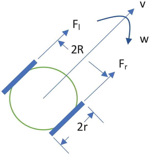
Differential-driven agricultural mobile robot.

There are two power wheels, one on the right and one on the left, to provide thrust and angular torque to the robot. The radius of the wheels is shown as r, and the radius of the robot is shown as R. Right motor wheel produces a force of F_r while the left motor wheel produces a force of F_l. The linear velocity of the robot is shown as v and the angular velocity is shown as w.

The outputs of the system are linear and angular velocities of the robot while inputs are torques produced by the motors of each wheel. So, the system is two input—two output system as shown in Figure 2.

Figure 2.

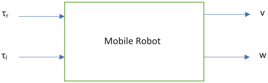
Mobile robot block diagram.

Applying Newton’s second law of motion for linear and angular motion of the robot:

F = m \frac{dv}{dt}

(1)

τ = J \frac{dw}{dt}

(2)

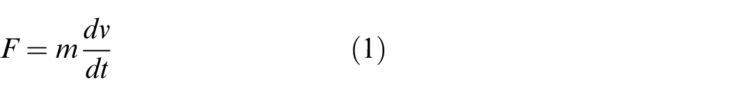
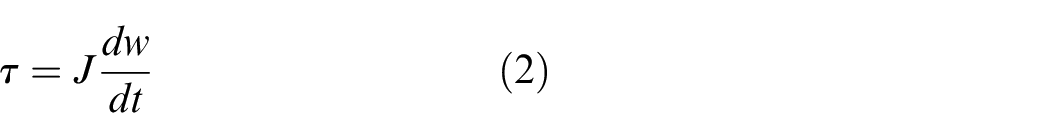
where F is the total linear thrust force, m is the total mass of the robot, v is the linear velocity, τ is the total angular torque, J is the inertia of the robot, and w is the angular velocity.

Linear thrust force and angular torque are calculated using the following formulas:

F = F_{r} + F_{l}

(3)

τ = (F_{r} - F_{l}) R

(4)

F_{r} = \frac{τ_{r}}{r}, F_{l} = \frac{τ_{l}}{r}

(5)

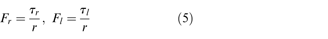
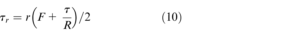
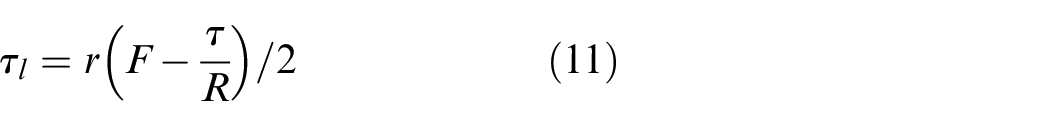
where r is the radius of the wheels, R is the radius of the robot, and τ_r and τ_l are right and left torques generated by corresponding motors, respectively.

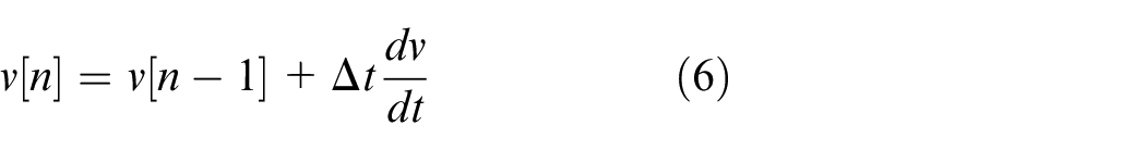
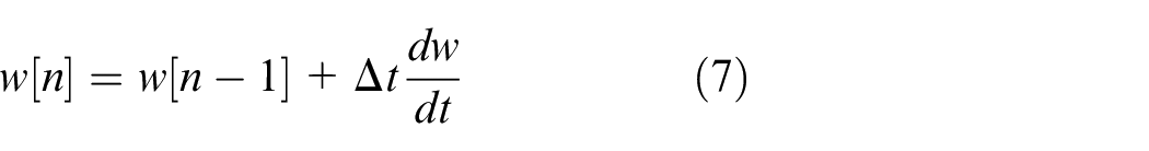
In the simulation, the trapezoid rule is used to calculate new values from old values and the derivatives.

v [n] = v [n - 1] + Δ t \frac{dv}{dt}

(6)

w [n] = w [n - 1] + Δ t \frac{dw}{dt}

(7)

Closed-loop control

The variables to be controlled in this system are linear and angular velocities. These are the outputs of the mobile robot system. It is desired that the outputs are regulated at certain values or track certain trajectories. This aim is achieved by continuously measuring and comparing output values with desired values and giving necessary inputs to the system, namely right and left wheel motor torques so that the outputs are kept at desired values. These necessary input torques are computed by the controller of the system. The Block diagram of the closed-loop control system is given in Figure 3. Note that one important contribution of this study is that reference and measured output information are given separately to the controller. This is different from most of the controller structures in the literature where only the error information is fed as input to the controller. There are some studies that use reference and error information but to our best knowledge this study is novel in the sense that windowed histories of both reference and measured output are fed independently and separately as input to the controller to calculate the control signal.2.3.

Figure 3.

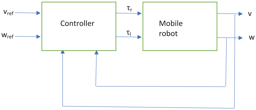
Closed-loop control system.

PID control

By far the most extensively used control system in the industry is the PID controller. In the PID controller, the control signal is computed using combinations of three components, namely proportional, integral, and derivative as the name implies. The formula of the PID controller for the agricultural mobile robot is as follows:

F = K_{pv} e_{v} + K_{iv} \int e_{v} dt + K_{dv} \frac{{de}_{v}}{dt}

(8)

τ = K_{pw} e_{w} + K_{iw} \int e_{w} dt + K_{dw} \frac{{de}_{w}}{dt}

(9)

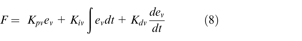
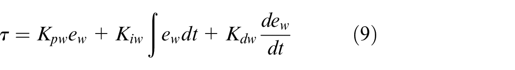
After the necessary intermediate values, F and τ, are computed, the necessary input values τ_r and τ_l are calculated with the following formulas:

τ_{r} = r (F + \frac{τ}{R}) / 2

(10)

τ_{l} = r (F - \frac{τ}{R}) / 2

(11)

PSO

PSO algorithm is used to find the parameters of the PID controller. In PSO, each hypothesis parameter value set is represented as a point in multi-dimensional parameter space. The number of points, namely particles, is a parameter of the algorithm to be determined and is important for the success of the algorithm. Too few points will result in suboptimal results found while too many points will make the computation unnecessarily slow. At the beginning of the PSO, each particle’s position and velocity are initialized to a random value within acceptable limits. After the random initialization of the particles, the position and velocity of each particle are calculated according to a well-established formula given below:

\begin{matrix} v [n] = c_{1} v [n - 1] + c_{2} (p [n - 1] - x [n - 1]) \\ + c_{3} (g [n - 1] - x [n - 1]) \end{matrix}

(12)

x [n] = x [n - 1] + v [n]

(13)

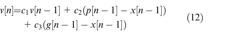
where v is the velocity of the particle, x is the position of the particle, p is the particle’s best-known position up to the current iteration, g is swarm’s best-known position up to the current iteration and c_i’s are constants to be determined as meta parameters of the algorithm.

In PSO optimized PID controller, the parameters of the PID controller are found using PSO algorithm. So, mathematically Kp, Ki and Kd of the PID controller are the parameters to be optimized:

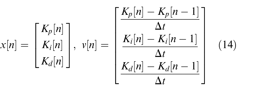
\begin{matrix} x [n] = [\begin{matrix} K_{p} [n] \\ K_{i} [n] \\ K_{d} [n] \end{matrix}], v [n] = [\begin{matrix} \frac{K_{p} [n] - K_{p} [n - 1]}{Δ t} \\ \frac{K_{i} [n] - K_{i} [n - 1]}{Δ t} \\ \frac{K_{d} [n] - K_{d} [n - 1]}{Δ t} \end{matrix}] \end{matrix}

(14)

These are the vectors x[n] and v[n] used in equations (12) and (13).

Single-layer neural-network controller

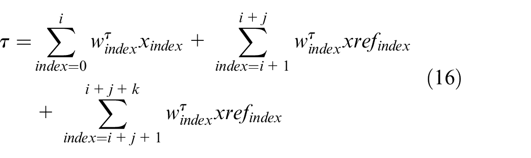
The proposed novel controller architecture consists of a single-layer neural network. The inputs to the network are past and current values of the outputs and past, current, and future values of the references. The outputs of the network are the necessary force and torque to be generated for the robot. The diagram of the proposed controller is given in Figure 4:

Figure 4.

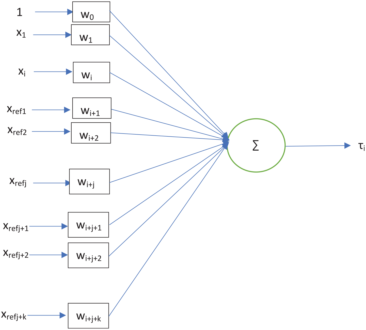
Proposed novel controller architecture.

Here, the inputs to the plant, namely force and torque to be generated for the robot, are calculated using the neural network structure. The inputs to the neural network are past and current values of measured velocities of the robot and past, current and future values of reference velocities of the robot. The outputs of the neural network are force and torque to be generated for the robot. So, the equations of the neural controller are as follows:

\begin{matrix} f = \sum_{index = 0}^{i} w_{index}^{f} x_{index} + \sum_{index = i + 1}^{i + j} w_{index}^{f} xre f_{index} \\ + \sum_{index = i + j + 1}^{i + j + k} w_{index}^{f} xre f_{index} \end{matrix}

(15)

\begin{matrix} τ = \sum_{index = 0}^{i} w_{index}^{τ} x_{index} + \sum_{index = i + 1}^{i + j} w_{index}^{τ} xre f_{index} \\ + \sum_{index = i + j + 1}^{i + j + k} w_{index}^{τ} xre f_{index} \end{matrix}

(16)

By using short histories of both reference and measured output signals and a short future history of reference signal, much more information is utilized to calculate the control signals and this results in enhanced performance as expected and reported in the results section.

Growing from PID equivalent controller

Note that number of parameters of proposed neural controller is much more than conventional optimal PID controllers. So, this results in a much higher dimensional parameter search space for training and finding optimum parameters of the controller. In order to make the training problem tractable, initial points are selected near to points equivalent to PID controller. This way a minimum performance equivalent to PID controller is guaranteed and the training converges to acceptable performance within acceptable time.

Results

Several experiments are conducted to prove the superiority of the proposed controller to the optimal PID controller. For small disturbance amplitudes, there is no important difference between performances but especially when the disturbance amplitudes are driven close to the saturation limits of the system, the proposed controller clearly shows better performance than the optimal PID controller.

All the simulations are done in Python programming language and Jupyter Notebook in the Anaconda environment.

Small disturbance: PID ≈ NN

For small disturbance amplitudes, the performance difference between the two approaches is small as shown in Figure 5.

Figure 5.

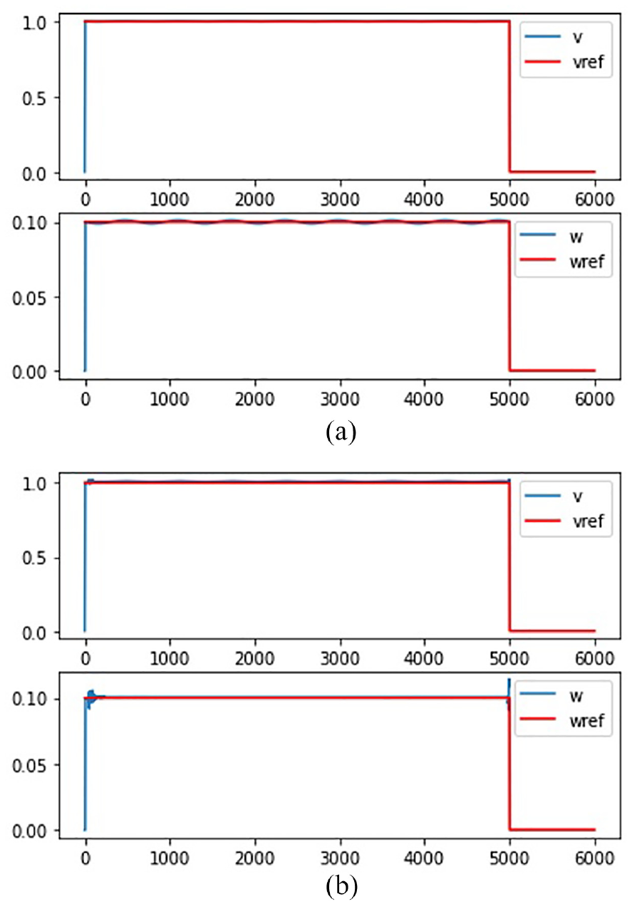
Performance comparison for disturbance amplitude of 1.5e0: (a) PID and (b) NN.

The performance of PID is about 2118 while that of NN is about 2607. Note that for small disturbance amplitude, the PID controller also shows acceptable performance. As the amplitude of the disturbance grows, the performance difference becomes more and more visible.

Step reference, sine disturbance: NN > PID

For greater disturbance amplitude, the performance difference becomes clearly visible as shown in Figure 6. The performance of PID is about 73 while that of NN is about 1470. Note that performance difference is clearly visible for angular velocity while that of linear velocity seems almost indistinguishable.

Figure 6.

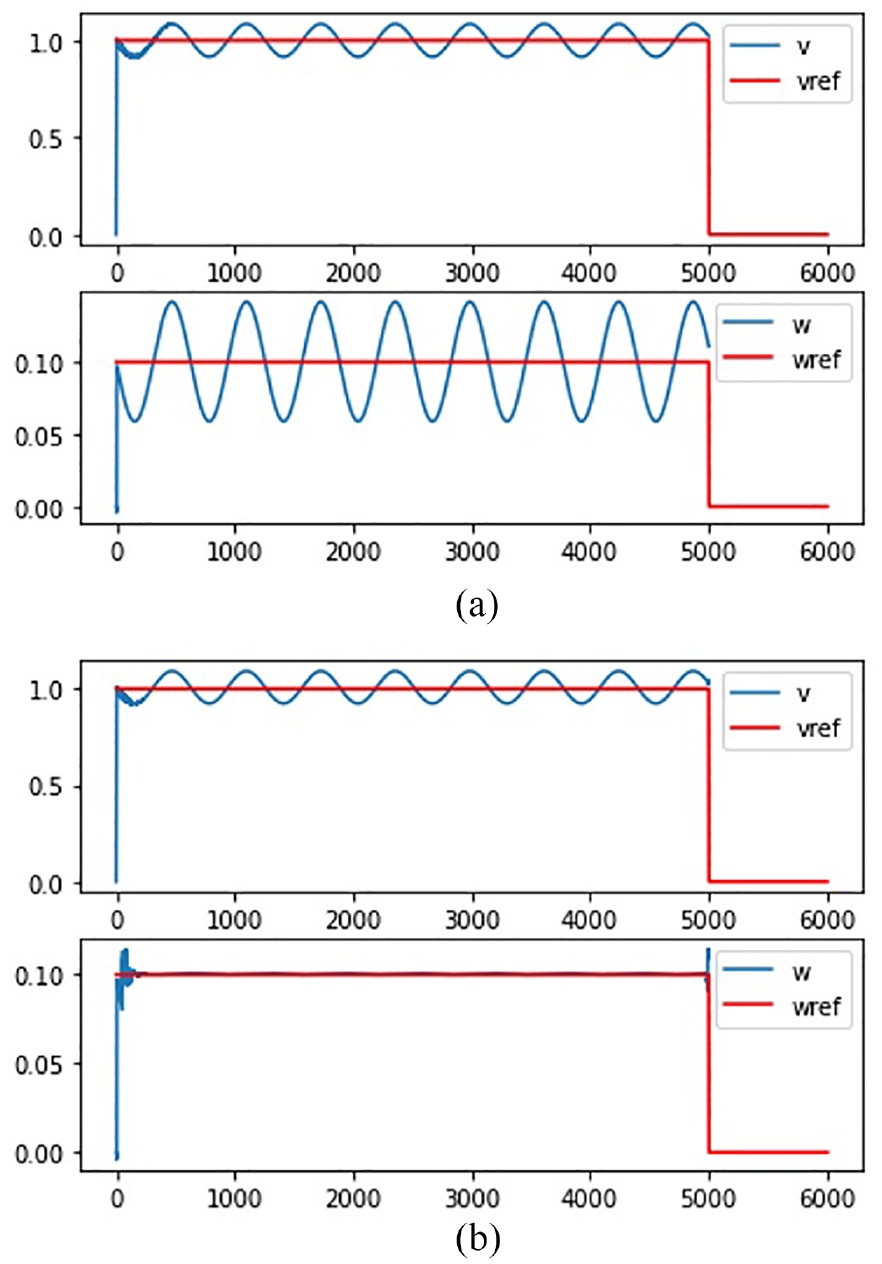
Performance comparison for disturbance amplitude of 4.95e1: (a) PID and (b) NN.

Sine reference, sine disturbance: NN > PID

For sinusoidal reference, the NN controller performs slightly better than the PID controller as shown in Figure 7. The performance of PID is about 74 while that of NN is about 93.

Figure 7.

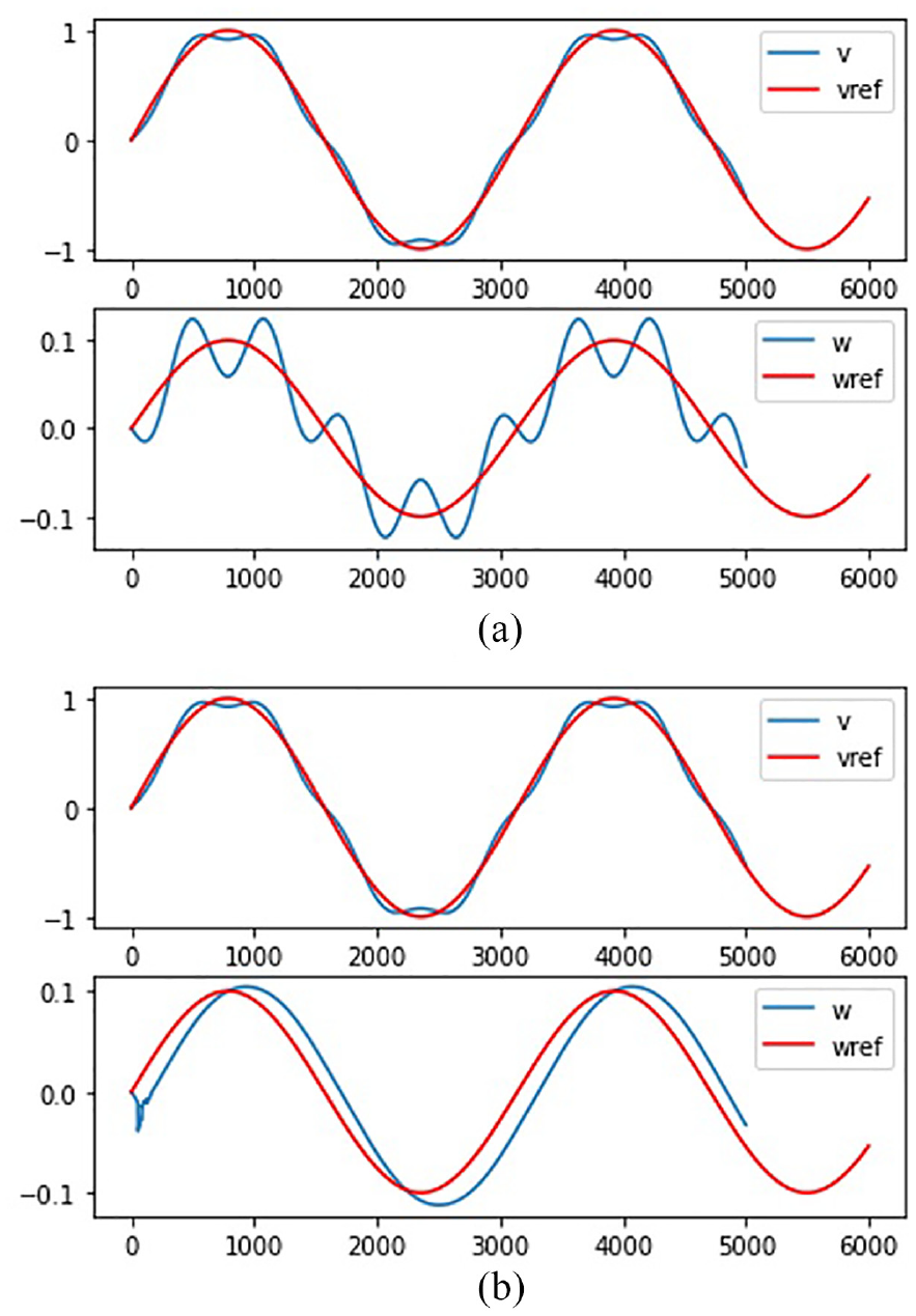
Sinusoidal reference: (a) PID and (b) NN.

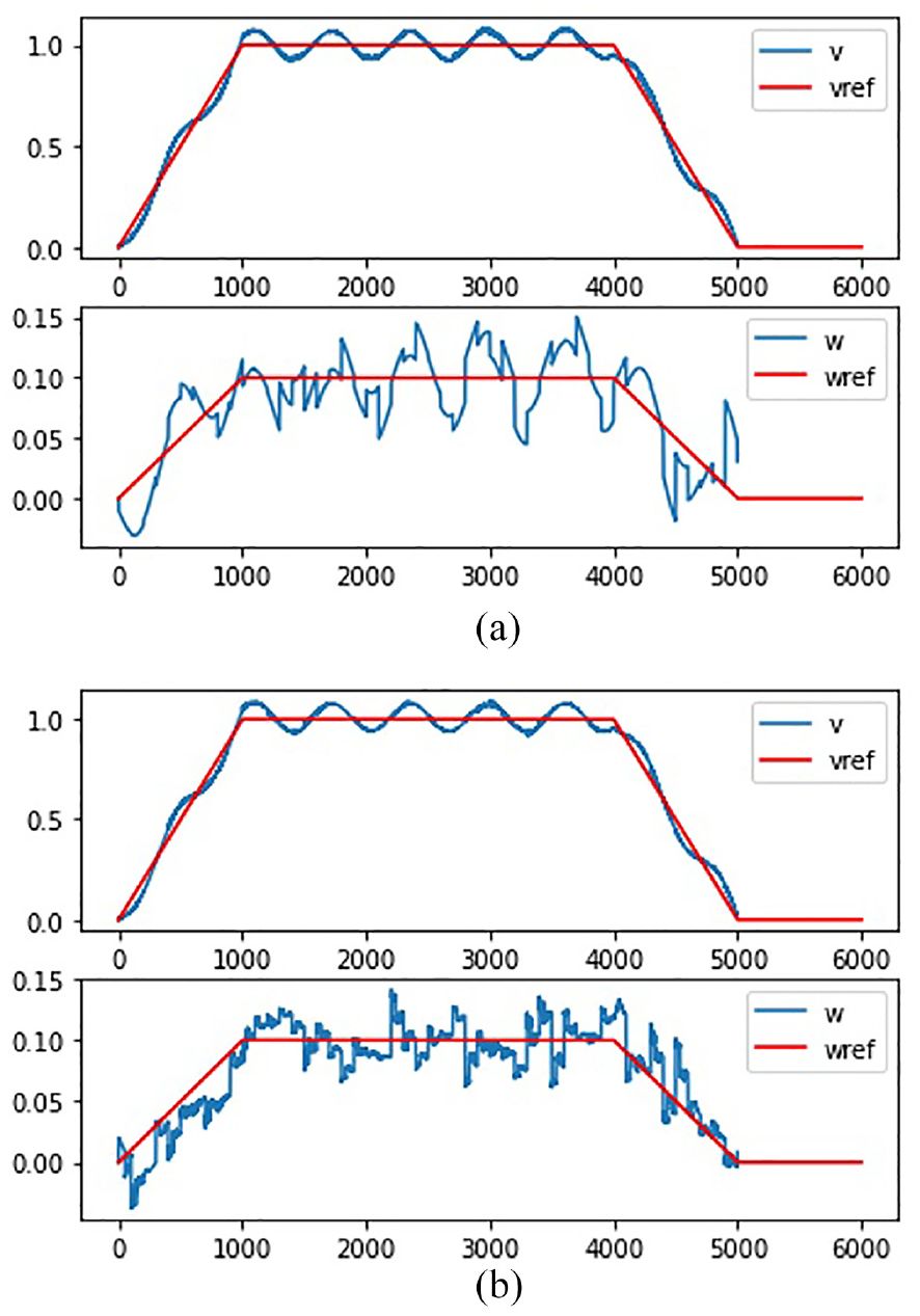
Trapezoid reference, sine disturbance: NN > PID

For trapezoidal reference, NN performs clearly better than PID as shown in Figure 8. The performance of PID is about 74 while that of NN is about 274.

Figure 8.

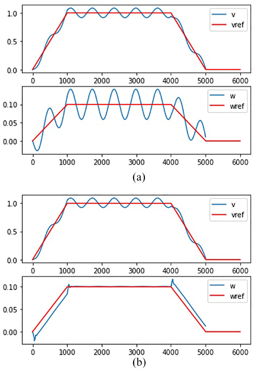
Trapezoid reference: (a) PID and (b) NN.

Trapezoid reference, sine plus random disturbance: NN > PID

The addition of a random component to the disturbance does not change the result too much. Still, the NN controller performs better than PID as shown in Figure 9 below. The performance of PID is about 90 while that of NN is about 130.

Figure 9.

Trapezoid reference, sinusoidal plus random disturbance: (a) PID and (b) NN.

Discussion

Note that in all cases the proposed single-layer neural network controller outperforms PID control. For small disturbance amplitude, the performance difference is small while as the disturbance grows, the difference between performances increases. This can be explained as follows: Neural network controller has much more parameters than that PID controller and hence is much more complex in terms of structure and functionality. A higher amplitude of disturbance means more effective input complexity. So, as disturbance amplitude grows, neural network complexity matches the complexity of input more. For high amplitude disturbance, the PID controller shows underfit due to low controller complexity.

Various types of inputs are tested in order to scan the input space more completely. In all types of inputs, the neural network controller outperforms PID control, also. Performance difference for step input seems more visible since step input has a wider range of frequency. One of the most used velocity reference types is trapezoid velocity reference and it is also shown that with trapezoid input neural network outperforms.

One important difference of the proposed controller is that information from reference and output is fed into the controller separately independent from each other. This enhances the information content of the controller input and is another important reason behind the increased performance. Note that especially in nonlinear systems like mobile robots, system behavior will be different for different values of inputs and depends not only on the difference but each value separately. Information from future reference input also is unique in the proposed controller so that the controller can anticipate the future needs of the system and adjust its output accordingly.

Another important novelty of the proposed controller is growing from an initially simple PID equivalent controller. This makes training time within tractable limits and guarantees at least the same performance as the initial point equivalent to the PID controller. Note that without PID equivalent controller initialization scheme, the search space of neural network based controller parameters is huge and an optimal solution cannot be found within acceptable training time. This second novelty is what makes proposed controller structure feasible.

Remarks

In machine learning field, it is known that complexity of the recognizer should match that of input for maximum generalization performance. With similar reasoning applied to intelligent control field, complexity of the controller should match that of disturbance expected. So, this is why the difference between performance of complex controller and simpler controller increases as disturbance becomes more complex.

Another important remark is as more information is used to calculate the control signal performance increases. So, additional information from reference and measured output improves the performance of the system.

Conclusion and future work

A differential-driven agricultural mobile robot is controlled using two different types of controllers and results are reported. Realistic system parameters are used for simulation. Various types of reference velocity references are given and outputs are observed. Neural network controller outperforms PID controller in all configurations of disturbance and inputs. Experimental results encourage the use of the proposed controller in especially highly nonlinear complex systems under complex and high amplitude disturbances.

In future work real robot experiments are planned to prove the validity of the proposed controller. Also, more complex multilayer neural network controllers are planned to be implemented and tested. Plants other than mobile robots are also planned to be tested. Various different starting points can be selected as initial parameters which would affect the final performance of the system and this could be another direction of future research.

Footnotes

Author contributions

Celal Onur Gökçe collected data, performed the experiments and analyses, and prepared the concept and design of the article.

Declaration of conflicting interests

The author declared no potential conflicts of interest with respect to the research, authorship, and/or publication of this article.

Funding

The author received no financial support for the research, authorship, and/or publication of this article.

Ethics approval

The study doesn’t need ethics approval.

ORCID iD

Celal Onur Gökçe

References

Tzafestas

. Mobile robot control and navigation: a global overview. J Intell Robot Syst 2018; 91(1): 35–58.

Pang

Liu

, et al. Adaptive sliding mode attitude control of two-wheel mobile robot with an integrated learning-based RBFNN approach. Neural Comput Appl 2022; 34: 14959–14969.

Eskander Dagher

Alaa Hameed

Amer Ibrahim

, et al. An adaptive neural control methodology design for dynamics mobile robot. Telkomnika 2022; 20(2): 392–404.

Zhang

Wang

. Reinforcement learning-based tracking control for a three mecanum wheeled mobile robot. IEEE Trans Neural Netw Learn Syst. Epub ahead of print 1 July 2022. DOI: 10.1109/TNNLS.2022.3185055.

Canbek

Yalcin

Baran

. Drift compensation of a holonomic mobile robot using recurrent neural networks. Intell Serv Robot 2022; 15: 399–409.

Liu

Cong

. Kinematic and dynamic control model of wheeled mobile robot under internet of things and neural network. J Supercomput 2022; 78(6): 8678–8707.

Janglová

. Neural networks in mobile robot motion. Int J Adv Robot Syst 2004; 1(1): 15–22.

Velagic

Osmic

Lacevic

. Neural network controller for mobile robot motion control. Int J Electr Comput Eng 2008; 3: 7.

Penar

Hendzel

. Experimental verification of the differential games and H∞ theory in tracking control of a wheeled mobile robot. J Intell Robot Syst 2022; 104: 61.

10.

Yang

Mita

, et al. Nonlinear tracking control of a car-like mobile robot via dynamic feedback linearization. In: Proceedings of the control 2004 conference, University of Bath, UK, September, 2004.

11.

DeVon

Bretl

. Kinematic and dynamic control of a wheeled mobile robot. In: 2007 IEEE/RSJ international conference on intelligent robots and systems, San Diego, CA, 29 October–2 November 2007, pp.4065–4070. New York, NY: IEEE.

12.

Astolfi

. Exponential stabilization of a wheeled mobile robot via discontinuous control. J Dyn Syst Meas Control 1999; 121(1): 121–126.

13.

Tayebi

Tadjine

Rachid

. Invariant manifold approach for the stabilization of nonholonomic chained systems: application to a mobile robot. Nonlinear Dyn 2001; 24(2): 167–181.

14.

Tian

Sidek

Sarkar

. Modeling and control of a nonholonomic wheeled mobile robot with wheel slip dynamics. In: 2009 IEEE symposium on computational intelligence in control and automation, Nashville, TN, 30 March–2 April 2009, pp.7–14. New York, NY: IEEE.

15.

Chang

Huang

. Nonlinear control of a wheeled mobile robot with nonholonomic constraints. In: 2004 IEEE international conference on systems, man and cybernetics (IEEE Cat. No. 04CH37583), Hague, The Netherlands, 10–13 October 2004, vol. 6, pp.5404–5410. New York, NY: IEEE.

16.

Ashoorirad

Barzamini

Afshar

, et al. Model reference adaptive path following for wheeled mobile robots. In: 2006 international conference on information and automation, 15–17 December 2006, pp.289–294. New York, NY: IEEE.

17.

Rigatos

Tzafestas

. Mobile robot motion control in partially unknown environments using a sliding-mode fuzzy-logic controller. Rob Auton Syst 2000; 33(1): 1–11.

18.

Tzafestas

Deliparaschos

Moustris

. Fuzzy logic path tracking control for autonomous non-holonomic mobile robots: design of system on a chip. Rob Auton Syst 2010; 58(8): 1017–1027.

19.

Das

Kar

. Design and implementation of an adaptive fuzzy logic-based controller for wheeled mobile robots. IEEE Trans Control Syst Technol 2006; 14(3): 501–510.

20.

Altan

. Performance of metaheuristic optimization algorithms based on swarm intelligence in attitude and altitude control of unmanned aerial vehicle for path following. In: 2020 4th international symposium on multidisciplinary studies and innovative technologies (ISMSIT), Istanbul, Turkey, 22–24 October 2020, pp.1–6. New York, NY: IEEE.

21.

Altan

Aslan

Hacıoğlu

. (2018, October). Real-time control based on NARX neural network of hexarotor UAV with load transporting system for path tracking. In 2018 6th international conference on control engineering & information technology (CEIT) (pp. 1-6). IEEE.

22.

Slama

Errachdi

Benrejeb

. Neural adaptive PID and neural indirect adaptive control switch controller for nonlinear MIMO systems. Math Prob Eng 2019; 2019; 7340392.

23.

Slama

Errachdi

Benrejeb

. Adaptive PID controller based on neural networks for MIMO nonlinear systems. J Theor Appl Inf Technol 2019; 97(2): 361–371.

24.

Mondal

Ray

Reddy

, et al. Intelligent controller for nonholonomic wheeled mobile robot: a fuzzy path following combination. Math Comput Simul 2022; 193: 533–555.

25.

Thai

TTK

Dzung

. Q: trajectory tracking control for differential-drive mobile robot by a variable parameter PID controller. Int J Mech Eng Rob Res 2022; 11(8): 614–621.

26.

Cao

Yang

, et al. Trajectory tracking control for a wheel mobile robot on rough and uneven ground. Mechatronics 2022; 83: 102741.

Single-layer neural-network based control of agricultural mobile robot

Abstract

Keywords

Introduction

Materials and methods

Mathematical model of agricultural mobile robot

Closed-loop control

PID control

PSO

Single-layer neural-network controller

Growing from PID equivalent controller

Results

Small disturbance: PID ≈ NN

Step reference, sine disturbance: NN > PID

Sine reference, sine disturbance: NN > PID

Trapezoid reference, sine disturbance: NN > PID

Trapezoid reference, sine plus random disturbance: NN > PID

Discussion

Remarks

Conclusion and future work

Footnotes

Author contributions

Declaration of conflicting interests

Funding

Ethics approval

ORCID iD

References