
Abstract
In view of that the tracking error originates from the amplitude attenuation and phase lag of the setpoints frequency component caused by the servo control system at each moment, this paper puts forward the idea of obtaining the setpoints time-frequency response (STFR) by solving the amplitude attenuation and phase lag of each frequency component of the setpoints at each moment. First, the feasibility of the proposed idea is proved theoretically; Then, the setpoints time-frequency transform is carried out and the solving method of STFR and setpoints time-frequency response error (STFRE) is established; Finally, taking the servo control system as the object, the STFR and STFRE are solved, and the corresponding relationship with the output time-frequency transformation and tracking error is analyzed to verify the proposed method. The contributions of the proposed method are: the method achieves the solution of STFR based on the amplitude attenuation and phase lag of the servo system; it avoids the limitation that only harmonic wavelet bases must be used in the existing method and can be applied to the solution of the time-frequency response of actual setpoints; it can separate the setpoints loss or tracking error caused by amplitude attenuation and phase lag; it can determine the redundancy or lack of strategies such as filters for certain setpoints and servo control system.
Introduction
Continuous trajectory control is one of the basic research fields of motion control. In order to control the contour error of continuous trajectory, the response of each axis servo system to the input setpoints must be sufficiently precise or coordinated at each position (or at each time of movement). The analysis of the formation mechanism of tracking error at each moment and the response process of the servo system to the setpoint at each moment is important for the control of continuous trajectory profile error.
The amplitude-frequency and phase-frequency characteristics of the servo control system profoundly explain the mechanism of the tracking error from the perspective of frequency-domain, that is, the tracking error at each time originates from the amplitude attenuation and phase lag of the frequency components of the setpoints at each time by the servo control system. Accordingly, the research on control strategies for tracking errors are mainly from the frequency-domain perspective, focusing on the servo control characteristics of the servo control system itself and the setpoints inputted to the servo control system.
Focusing on the servo control characteristics, the feedforward controller, 1 notch filter, 2 modal filter, 3 and sliding mode controller 4 can greatly improve the amplitude-frequency characteristics and phase-frequency characteristics and hence significantly reduce the tracking error. Koren and Lo,5,6 Altintas et al., 7 and Lyu et al. 8 systematically summarized the research progress in each period. Around the setpoints inputted to the servo control system, the frequency-domain analysis of the setpoints by FFT is the main method. Smith 9 and Altintas et al. 7 used fast Fourier transform (FFT) to analyze the frequency of different types of setpoints, and concluded that setpoints with acceleration second order continuous jerk have the least potential excitation frequencies and are most suitable for use as servo system inputs.
The magnitude of the tracking error is related not only to the servo control characteristics of the servo control system itself, but also to the setpoints inputted to the servo control system. The former can be considered not to change with time. However, the speed, acceleration and jerk of the setpoints change with time, resulting in that the tracking error presents a significant time-dependent characteristic. The frequency-domain characteristics of the servo control system and the FFT analysis of the setpoints do not have time information, which cannot focus on the specific time to analyze the time-dependent characteristic of the tracking error. Analyzing a servo control system from a time-domain perspective is a direct means to study the time-dependent characteristic of the tracking error. From a time-domain perspective, a servo control system needs to be described as a differential equation or transfer function. Servo system performance is measured using metrics such as overshoot, adjustment time, and rise time. The setpoints and system errors are then plotted as time-domain curves that allow visualizing the extremum values of velocity, acceleration and jerk to determine if the physical limits of the motor are exceeded.10–16 However, the analysis of tracking error from the time-domain perspective can only provide an intuitive view of the control effect and does not allow exploring new control strategies.
To sum up, no matter the frequency-domain analysis or time-domain analysis of the servo control system, it is not possible to quantitatively express the response process of the servo control system to the setpoints at each moment in the frequency domain. In general, the time domain analysis method and frequency domain analysis method are independent of each other and need to introduce the time-frequency analysis method.
Time-frequency analysis is a modern branch of harmonic analysis. It analyzes signal in both the time- and frequency- domain simultaneously, which is broadly studied and used in image processing, signal analysis and communication theory, and so on. However, in motion control, there are only a few related literatures so far. Rotariu et al. 17 introduced time-frequency analysis into motion control. They combined the time-frequency analysis of the Wigner distribution with the field of iterative learning control (ILC) and designed a time-frequency adaptive filter to control the wafer in ILC.18,19 The Wigner distribution was successfully used for tracking error control, demonstrating the feasibility and promise of time-frequency analysis for motion system analysis. Galleani 20 used the Wegener distribution to transform the motion control system from the time domain to the time-frequency domain so that the time-frequency spectrum of the system output can be calculated. This method achieves the solution of the time-frequency response by time-frequency transformation of the system, but the calculation of the time-frequency transformation of the system is very complicated. In order to simplify the time-frequency response solving method, it becomes another choice to realize the time-frequency response solving by time-frequency transformation of the setpoints. Tratskas and Spanos 21 proposed the introduction of wavelet transform to describe the excitation-response relation for multiple-input multiple-output systems in the time-frequency domain, and they successfully described the response process of a second-order system to a random input under the premise of harmonic wavelets as basis functions. Subsequently Spanos et al. 22 further optimized the effectiveness of the method in lightly damped systems and successfully derived the excitation-response relation in a single-degree-of-freedom linear structure. However, the method can only be used in the case where the wavelet basis is a harmonic wavelet basis. Harmonic wavelet basis has good smoothness, and has excellent performance when dealing with smooth signals, such as sine functions and spline functions. However, in the servo control system, the input setpoint signal often has discontinuous features such as start-stop, corner, and spike, so the application range of the method based on harmonic wavelet basis only is narrow. In order to realize the response solution for arbitrary input, we need to study a time-frequency response solution method that is not limited by the wavelet basis type.
In essence, the output of the servo control system has changed in amplitude and phase relative to the input. From this point, this paper proposes a method for solving the STFR of servo systems. First, the frequency component of setpoints at each time is characterized by time-frequency analysis method. Then, using the frequency-domain feature of servo control system, the amplitude and phase changes of the output of the servo control system relative to the input at each time are given. Finally, the STFR of the servo control system is approximated by integrating the time-frequency characterization of the setpoints and the amount of amplitude and phase change of the servo system to the setpoints.
Time-frequency transformation of setpoint
This section uses time-frequency analysis to transform setpoints from time-domain to time-frequency domain, and solves the frequency components of setpoints at each time.
The choice of time-frequency analysis methods needs to consider the characteristics of setpoints and the needs of analysis:
(1) The effective frequency component of the setpoints are mainly concentrated in the low frequency band, which requires high low frequency accuracy of the time-frequency analysis method. In addition, the frequency distribution range after time-frequency analysis needs to be able to cover the position loop bandwidth of the servo control system.
(2) The time resolution of the setpoints after the time-frequency analysis needs to be far lower than the processing time of conventional part trajectory.
The time-frequency analysis methods such as Wigner-Ville distribution (WVD) and Hilbert-Huang transform (HHT) give the time-frequency information of the signal based on the characteristics of the signal itself. Its frequency band division and frequency resolution are only related to the signal itself and cannot be adjusted actively. Continuous wavelet transform (CWT) divides the signal at each time into a set of artificially set frequency bands through the similarity between wavelet basis and signal components. Although CWT is slightly inferior to WVD and HHT in accuracy, it has initiative in setting frequency scale and time scale 23 which can be set according to the requirements of frequency resolution, frequency analysis range and time resolution.
The setpoints position sequence input to a servo control system is:

where, k is the number of interpolation cycles,
The CWT of the setpoints position sequence
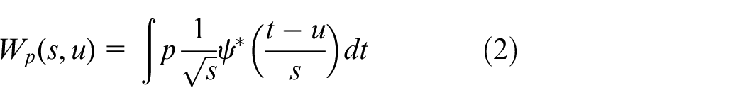
where,
Unless otherwise specified,
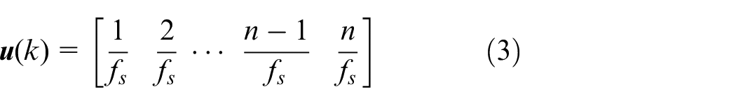
Where, k represents the position of the element in the sequence, and the value is an integer from 1 to n;
In order to correspond the scale factor
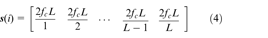
where, i represents the position of the element in the sequence, and the value is an integer from 1 to L,
The length L of the scale sequence determines the resolution of the frequency
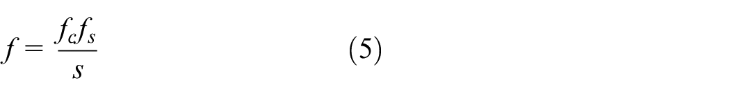
Substituting equation (4) into equation (5), the frequency sequence can be obtained as:
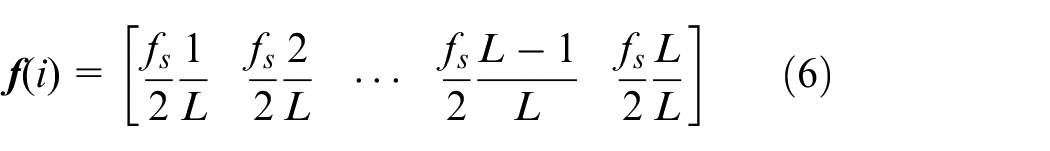
It can be seen from equation (6) that the frequency sequence
In the remaining examples of this paper, the wavelet basis function
Through equations (2)–(6), CWT can be carried out on the setpoints position sequence, as shown in equation (7).
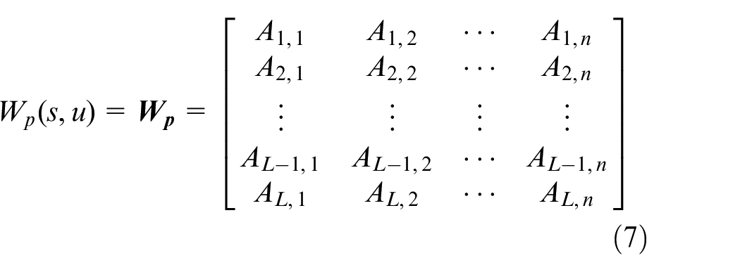
where,
Equation (7) transforms the setpoints from time-domain to frequency-domain, expressed as time-frequency matrix. The rows and columns in the matrix correspond to frequency and time, respectively. The values of the elements in the matrix are wavelet coefficients, which can be regarded as the setpoints amplitude. The smaller the wavelet coefficient, the smaller the setpoints amplitude in the corresponding frequency and time.
Solving idea and feasibility theory proof of STFR
The frequency-domain characteristic characterizes the response ability of the servo control system to the setpoints. Among them, the amplitude-frequency characteristic represents the amplitude attenuation of each frequency component of the setpoints by the servo control system; The phase-frequency characteristic represents the phase lag of the servo control system to each frequency component of the setpoints. Through CWT, the frequency components of the setpoints at each time are obtained. Combined with the connotation of frequency-domain characteristics of servo control system, this section puts forward the idea of solving the STFR by solving the amplitude attenuation and phase lag of setpoints frequency components at each time. Next, the feasibility of the proposed solution is proved theoretically.
CWT has the following properties:
(1) CWT is a kind of linear transform, which can be superimposed. If the CWT of

(2) CWT has translation. If the CWT of
With a linear time-invariant servo control system
Rewrite the equation (7) of the position setpoints
where,
For any CWT that satisfies the wavelet admissibility condition, there is its inverse transform which can be expressed as:
Where,
Substituting the time sequence
Where,
At this time, the original setpoints position
Since
where,
Because
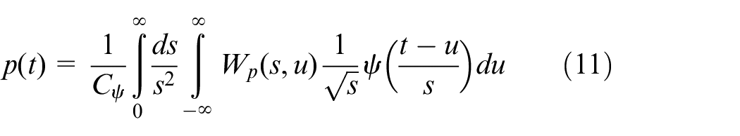
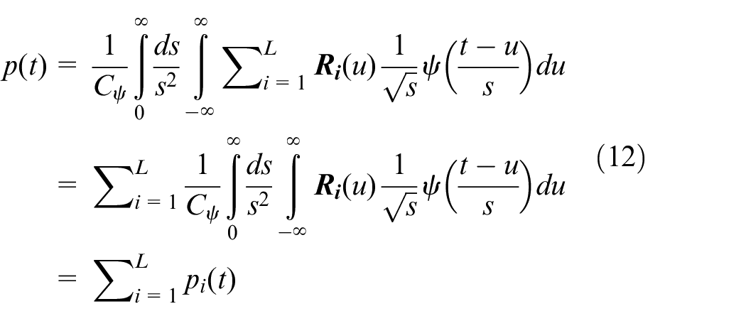
From equation (12),
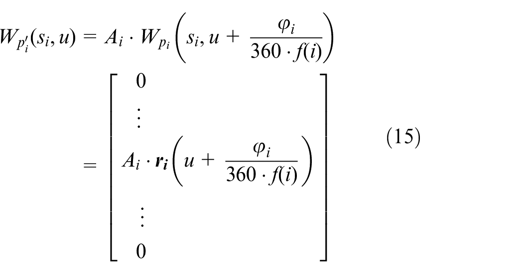
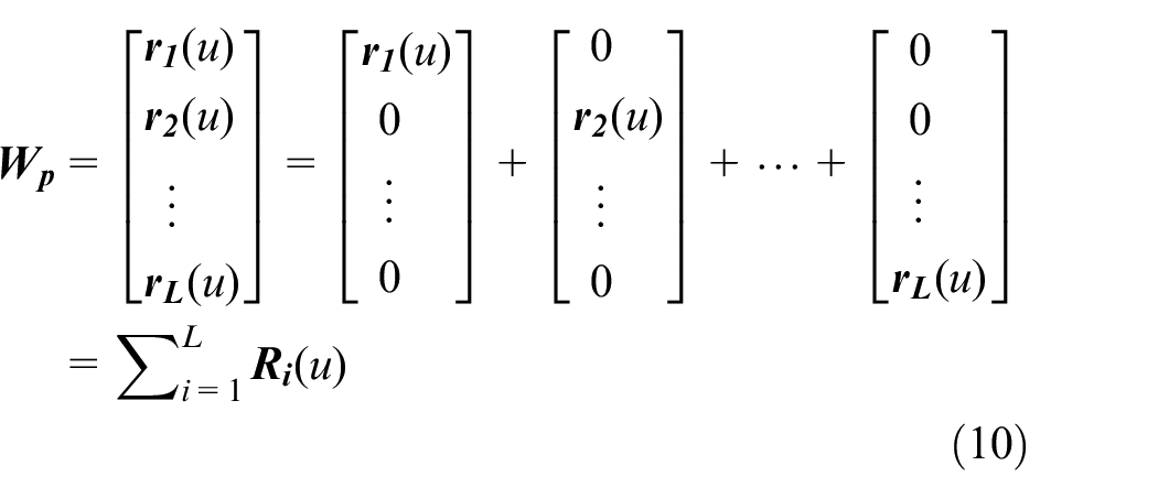
According to equation (14) and the superposition characteristics of wavelet, the wavelet transform
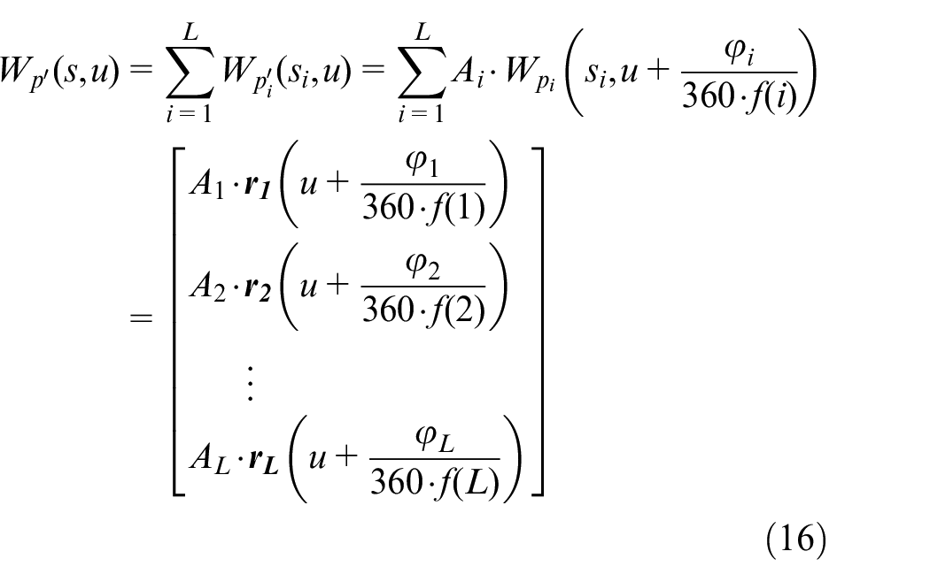
where,
Equation (16) decomposes a sequence of setpoints into multiple ideal single frequency signals by using CWT, and solves the response of each single frequency signal according to the frequency-domain characteristics of the servo control system. The method is carried out in a linear premise, and obviously, the entire solution process wavelet basis function does not require a specific representation.
Solving method of STFR
The essence of equation (16) is to use the frequency-domain characteristics of the servo control system to carry out amplitude attenuation and time lag for different frequency components obtained by the CWT of the setpoints. This solution requires not only wavelet transform of setpoints, but also conversion of frequency-domain characteristics of servo control system into amplitude attenuation and time lag. Frequency-domain characteristics of servo control system are generally represented by Bode diagram. In order to express equation (16) in the form of a practically usable discrete matrix, in this section, the amplitude attenuation ratio expression is constructed based on the amplitude-frequency characteristics and the lag time expression is constructed based on the phase-frequency characteristics of the Bode diagram.
Establishment of discrete expression of amplitude attenuation ratio (AAR)
According to the definition of unit of amplitude (decibel) of amplitude-frequency characteristic, the amplitude-frequency characteristic can be converted into an expression of AAR, that is the ratio of output amplitude to input amplitude, as shown in equation (17).
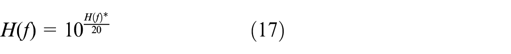
where,
In the amplitude-frequency characteristic, take the frequency range
where,
Establishment of discrete expression of Lag Time (LT)
Convert the phase-frequency characteristic of Bode diagram into LT, as shown in equation (19).
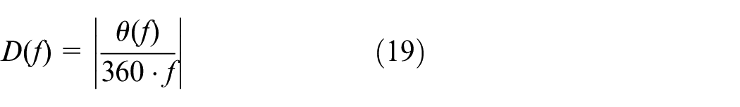
where,
In the phase-frequency curve, take the frequency range

where,
Solving method flow of STFR
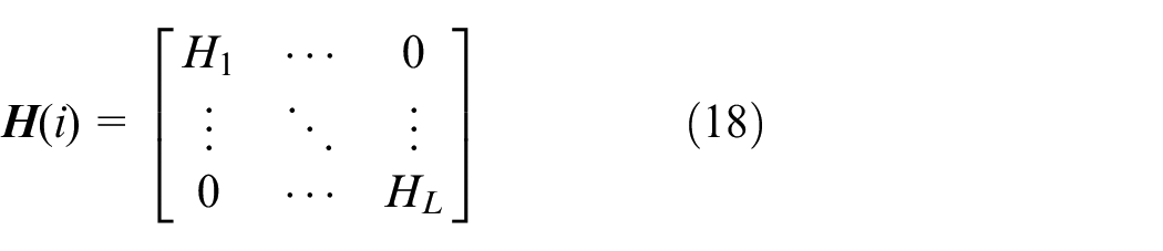
Equation (17) expresses the AAR at different frequencies. The attenuation effect of the servo control system is equivalent to scaling the setpoints time-frequency matrix according to the amplitude-frequency characteristics of the servo control system, that is, each row element of equation (7) is attenuated according to equation (18). Therefore, the attenuated STFR can be expressed as
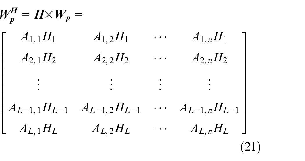
where,
According to the translation of wavelet transform, the wavelet coefficients of the delayed signal can be obtained by translating the wavelet coefficients of the original signal in the time sequence

After time lag as shown in equation (22), the STFR
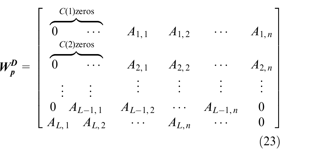
where,
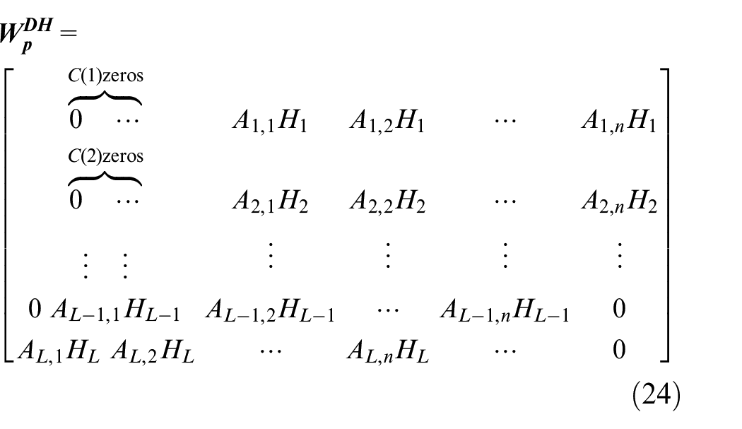
Combining equations (21) and (23), the STFR attenuated and lagged by the servo control system can be obtained, which is expressed in matrix form
Definition and solving method of STFRE
Setpoints loss (SL)
In the research and application of servo control, attention should be paid not only to response, but also to error. The amplitude attenuation and phase lag of the servo control system to the setpoints results in a difference between the input and output, that is, SL. When expressing this loss in the time-frequency domain, it is referred to as STFRE.
By subtracting the time-frequency matrix of the original setpoints from the time-frequency matrix of the response, that is, equations (24) and (7), the difference matrix
where,
Time lag leads to an increase in the number of
According to Moyal’s theorem, the integral of the wavelet coefficient square is proportional to the energy of the signal, and this proportional coefficient is related to the choice of wavelet basis. It means that although the wavelet coefficient is positively correlated with the amplitude of the signal, the value of the wavelet coefficient will change with the change of the wavelet basis function. Therefore,
where
When establishing the SL matrix, normalization processing is carried out. However, since the AAR applied in calculating the setpoints response is already a ratio, simple normalization will make the SL only related to the amplitude frequency characteristics and independent of the setpoints itself, which will lead to the inconsistency between the loss of high-frequency part and its actual amplitude. Therefore, the adjustment coefficients
In equation (26), if
Setpoints loss at each time (SLET)
The frequency integral of equation (26) is defined as the SLEL
In equation (27),
Equation (21) establishes the setpoints time-frequency matrix
Setpoints loss at each frequency (SLEF)
The time integral of equation (26) is defined as the SLEF
In equation (28),
Verification
This section establishes the servo control model and designs the verification scheme to verify the solving methods for the STFR and the STFRE.
Servo control model and its AAR and LT
The servo dynamic model of x-axis of three-axis vertical milling machine established by Lyu et al. 24 is adopted for verifying the solving method. In this model, the feed system is equivalent to a four rigid body dynamic model, as shown in Figure 1.
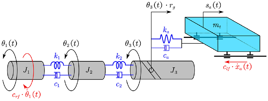
The dynamic model of the x-axis of three-axis vertical milling machine.
The dynamic equation is shown in equation (29).

where,
The control block diagram of the servo control system is shown in Figure 2. The current loop is equivalent to the first-order inertia element, the speed loop adopts PI control and the position loop adopts P control. On this basis, the speed feedforward controller is added.
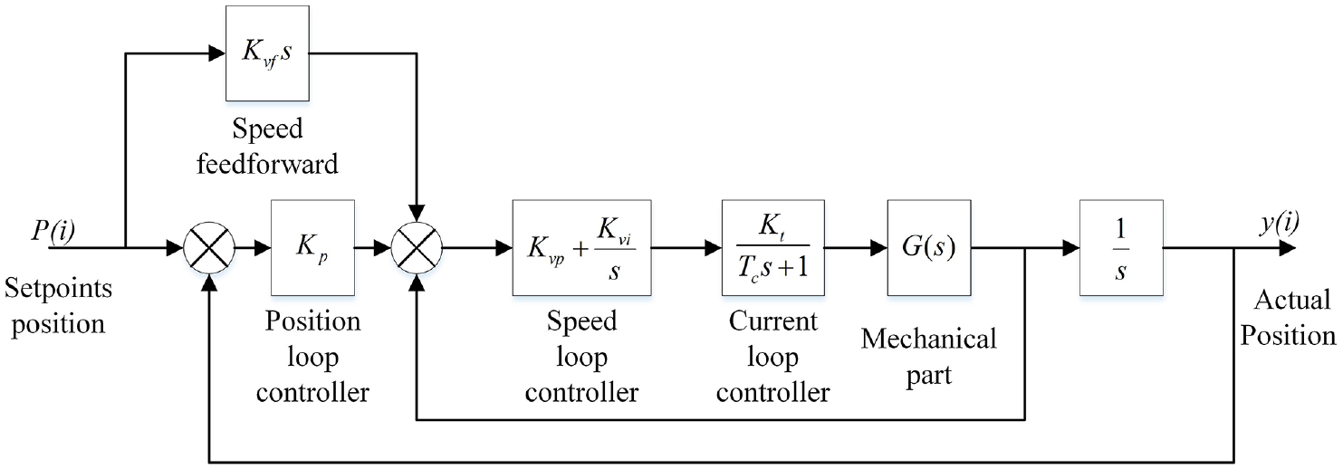
The control block diagram of the servo control system.
The speed loop transfer function is shown in equation (30):
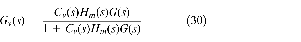
where,
The position loop transfer function of the servo control system is shown in equation (31).
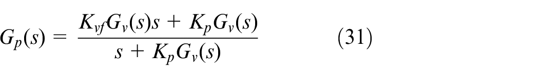
where,
The Bode diagram of the servo control system is drawn according to equation (31), as shown in Figure 3.
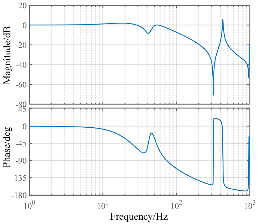
The position loop Bode diagram of the servo control model.
According to equations (17) and (19), the AAR and LT of the servo control system are established, as shown in Figure 4.
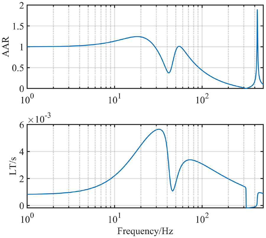
The AAR and LT at each frequency point.
Verification of the solving method for the STFR
Verification scheme
In this subsection, a basic signal is constructed, and the time-frequency response matrix of the signal is obtained by the proposed method and simulation experiments to verify STFR solution method, respectively.
Sinusoidal signal is a basic signal with the simplest frequency component. For the signal superimposed by sinusoidal signals of multiple frequencies, the components of frequencies can be well separated in the time-frequency diagram. Therefore, sinusoidal signals are used to verify the solving method of the STFR.
The signal expressed as equation (32) are designed as the setpoints inputted to the servo control system:

The signal includes three frequency components: 8, 20, and 40 Hz, and its amplitude are set to 1. The total duration of the signal is 2.5 s and the output frequency is 4000 Hz.
The designed verification scheme is as follows:
(1) Calculate the time-frequency matrix of the signal described in equation (32), mark the sample points from it, and record their values and positions.
(2) Input the signal described in equation (32) into the servo control model established in Section 6.1 to obtain the output signal. Calculate the time-frequency matrix of the output signal, and record the value and position of sample points in the output time-frequency matrix as the standard value.
(3) Use the STFR solving method described in Section 4 to solve the STFR matrix. Record the value and position of sample points after attenuation and lag as the calculated value.
(4) Compare the calculated values with the standard values to verify the solving method.
Verification results
Input
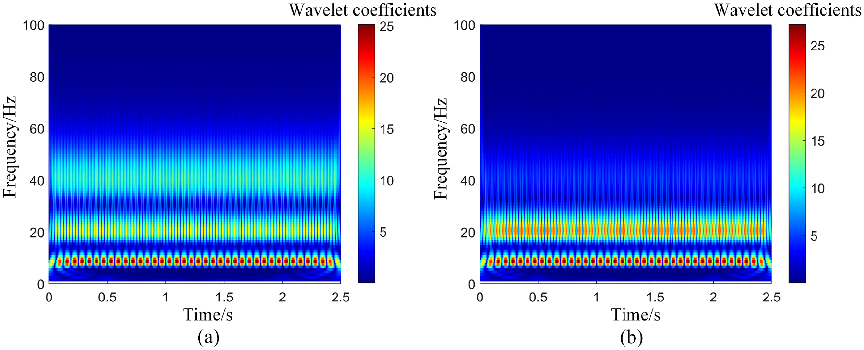
The time-frequency diagrams of input and output signals: (a) time frequency matrix of input signal and (b) time frequency matrix of output signal.
In order to accurately locate the sample points in both the input time-frequency diagram and the output time-frequency diagram, it is necessary to select some easily distinguishable points as sample points.
For sinusoidal signal, after CWT, when the frequency remains unchanged, the variation law of wavelet coefficient with time is still sinusoidal curve, and the interval between peak points on the curve is half of the cycle of sinusoidal curve. Therefore, in the time-frequency matrix of
Sample point information.
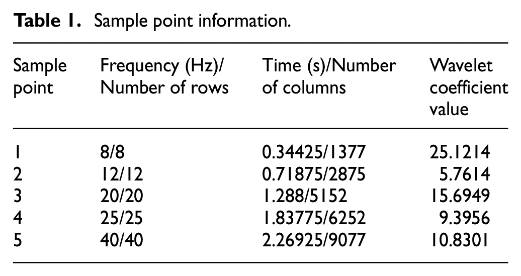
The position and wavelet coefficient value of the corresponding sample point in the time-frequency matrix of the output signal
Comparison of standard value and calculated value of each sample point.
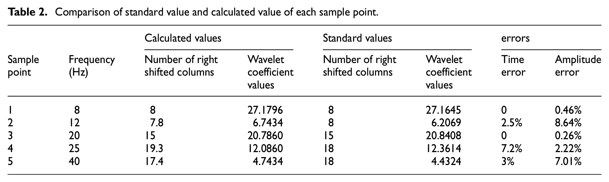
It can be seen from Table 2 that in sample points 1 and 3, the calculated values are very close to the standard values. However, there are some errors in sample points 2, 4, and 5. In the table, the number of columns shifted to the right represents the time lag. Because the sampling frequency of signal
Verification of the solving method for SLET
The SLET should have a corresponding relationship with the tracking error at each time. In this section, two motion trajectories are designed to analyze the SLET. Inputting the two trajectory setpoints into the servo control model established in section 6.1, the tracking errors can be calculated. The corresponding relationship between SLET and tracking error at each time is analyzed to verify the proposed method.
Trajectory design and time-frequency transformation of its setpoints
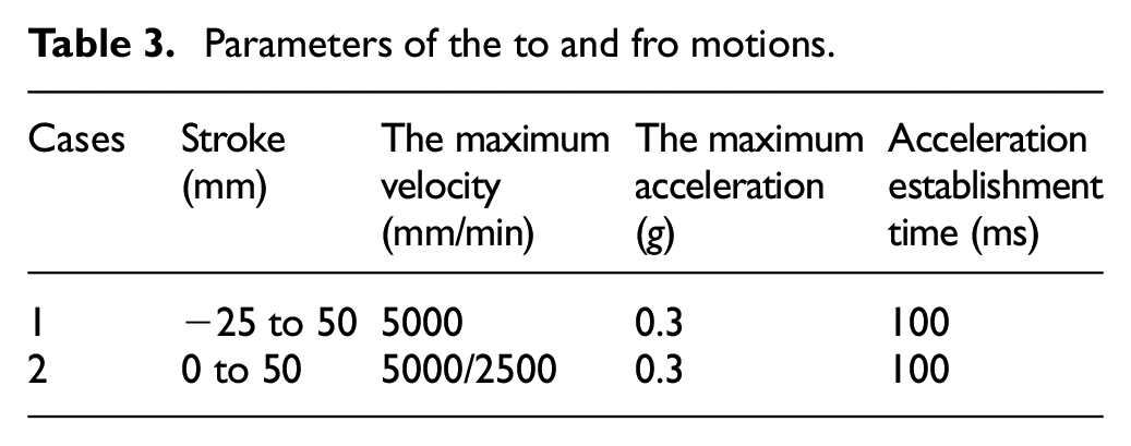
Taking the to and fro motions as examples, two cases with different motion parameters are designed to carried out the time-frequency transformation. The main parameters of the motions are shown in Table 3
Parameters of the to and fro motions.
The setpoints of the two motions are interpolated and collected by the KEDE GNC61 CNC system. The setpoints position, velocity and acceleration of the two motions are shown in Figure 6.
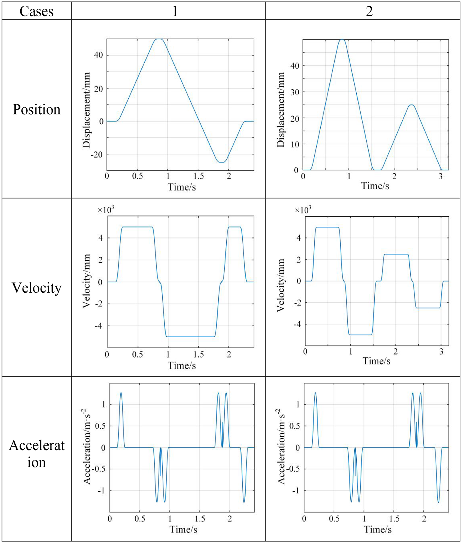
Setpoints position, velocity and acceleration curves of the two motions.
According to the method described in Section 2, the time-frequency analysis of setpoints position sequences is carried out to construct the setpoints time-frequency distribution matrix. The matrix is L row and n column, corresponding to the time sequence and frequency sequence shown in equations (3) and (6). The corresponding time-frequency distribution diagrams are drawn, as shown in Figure 7.
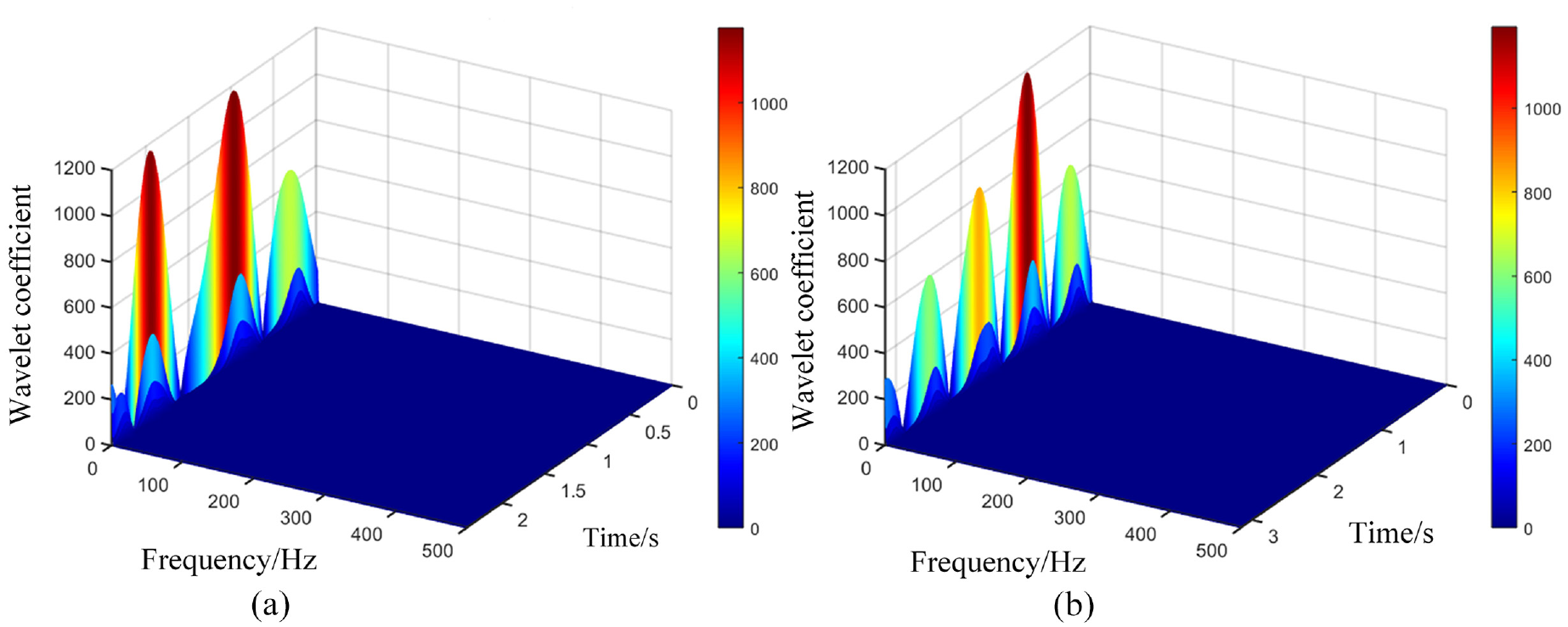
The time-frequency distribution diagrams of the setpoints of the two cases: (a) Case 1 and (b) Case 2.
Corresponding relationship between SLET and tracking error at each time
According to the method described in Section 5.2, the SLET
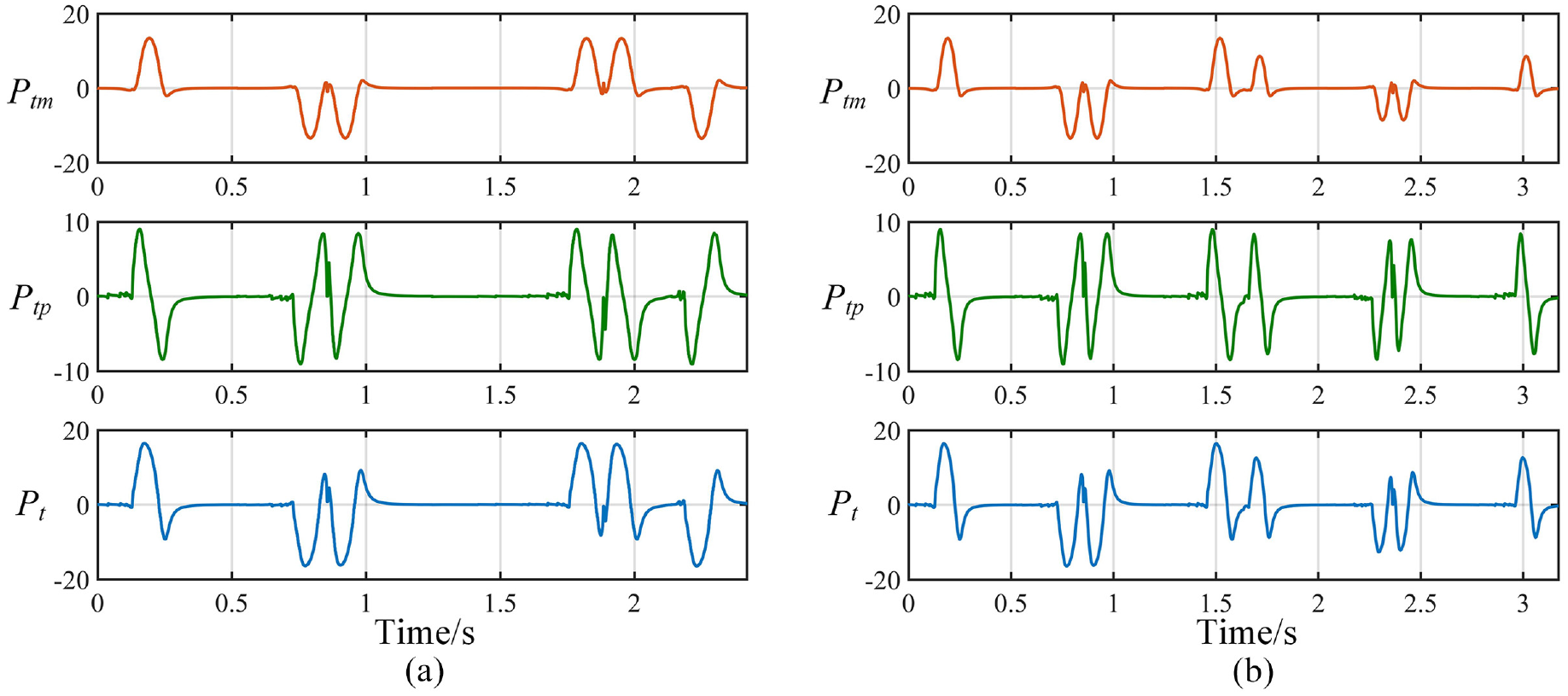
SLET of the two cases: (a)
The value of
In the inverse transformation equation (12), the derivative is derived for time on each side of the equal sign. The left side is the setpoints speed, while the right side is frequency integral of the product of wavelet coefficients and wavelet basis. Considering that the SL matrix in equation (26) is a relative quantity in the calculation of
The setpoints of the two cases are inputted into the servo control model established in Section 6.1 to obtain the speed tracking error. Figure 9 shows the speed tracking error and
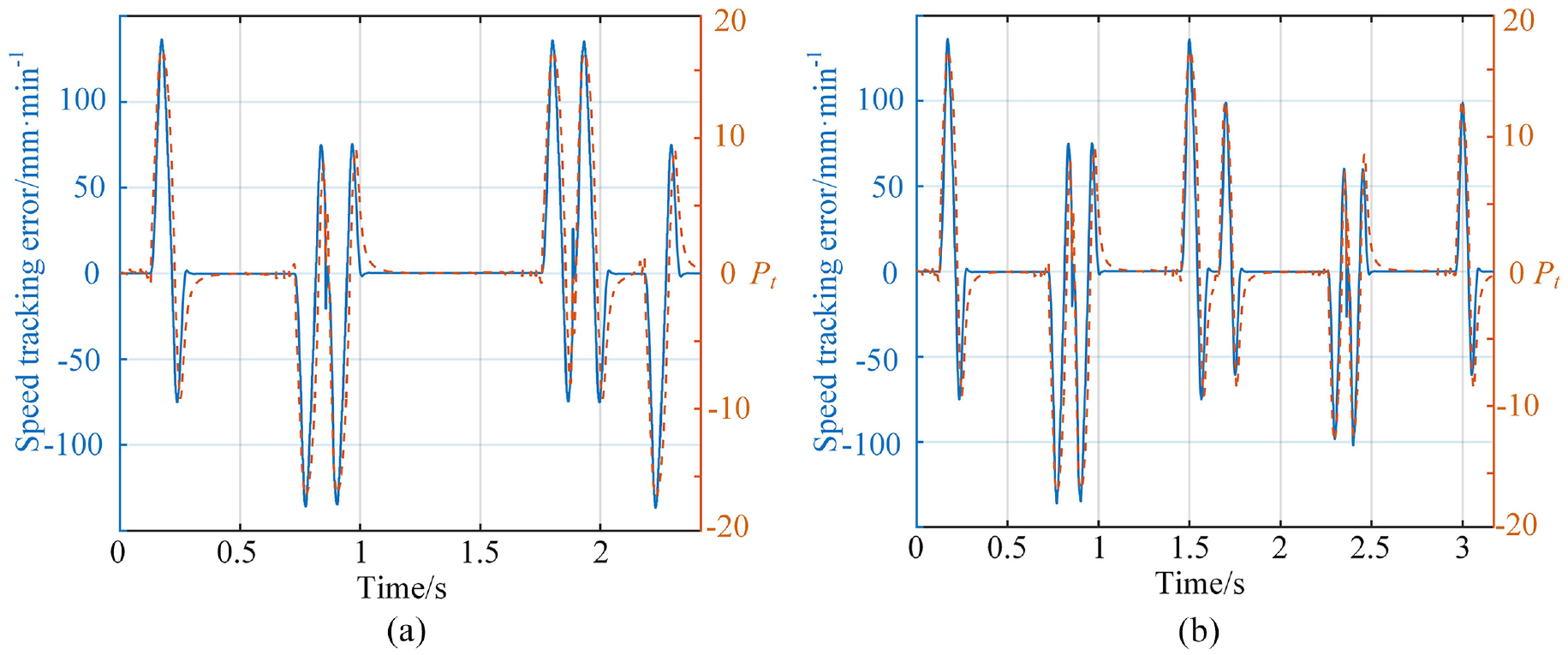
Comparison between speed tracking error and
Combined with the results of Figure 9, given that the initial value of trajectory displacement is 0, the integral of
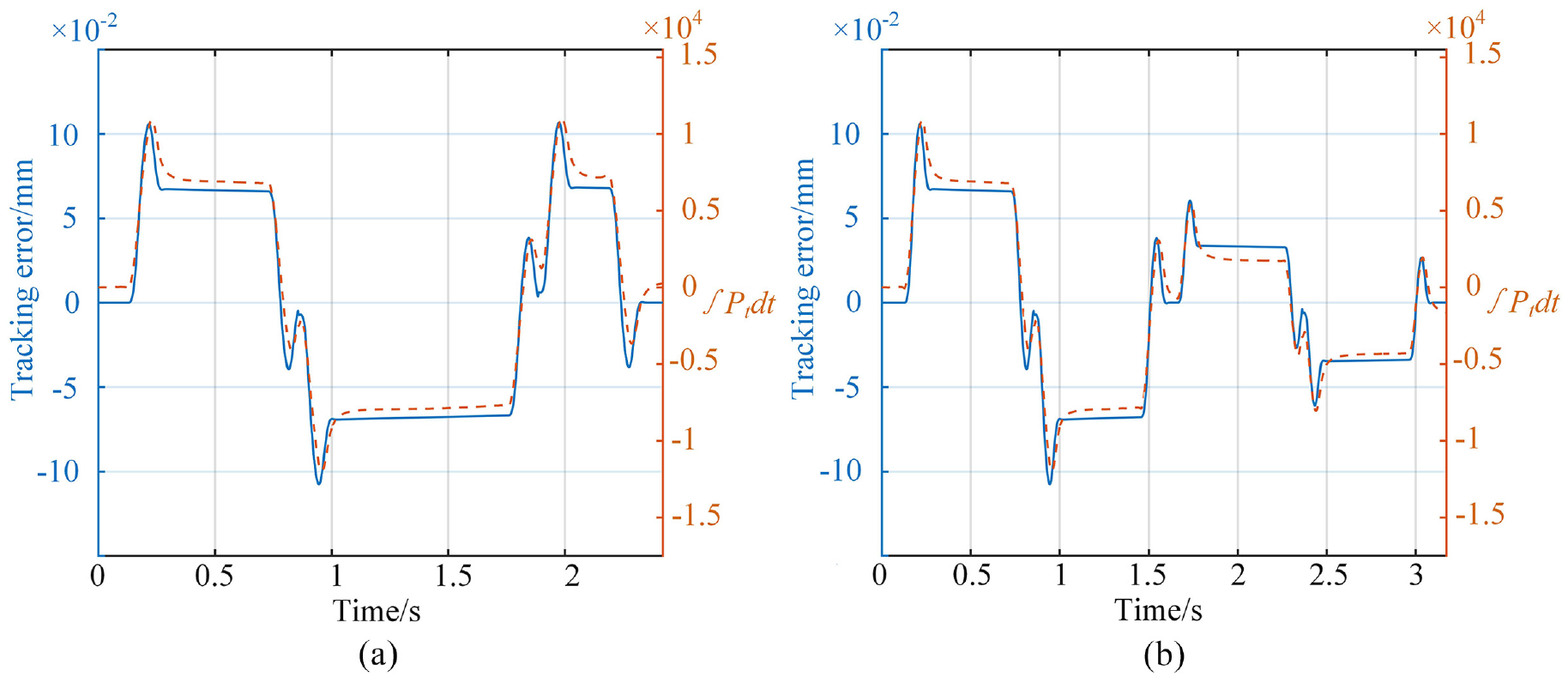
Comparison of position tracking error and
Tracking error under the action of amplitude attenuation or phase lag: (a) Case 1 and (b) Case 2.
Discussion
After the verification of the solving methods for STFR and STFRE, its theoretical significance and application prospect will be discussed in this section.
Theoretical significance of STFR and STFRE
Figure 12 shows the STFR diagram and STFRE diagram of the two cases. The diagrams of STFRE clearly show the SL at each time and the SL of each frequency. For a certain time, the loss of each frequency component is caused by the amplitude-frequency characteristics and phase-frequency characteristics of the servo control system. The SL at a certain time corresponds to the tracking error at that time. This analysis method realizes the unification of the time-domain phenomenon and frequency-domain mechanism of the tracking error.
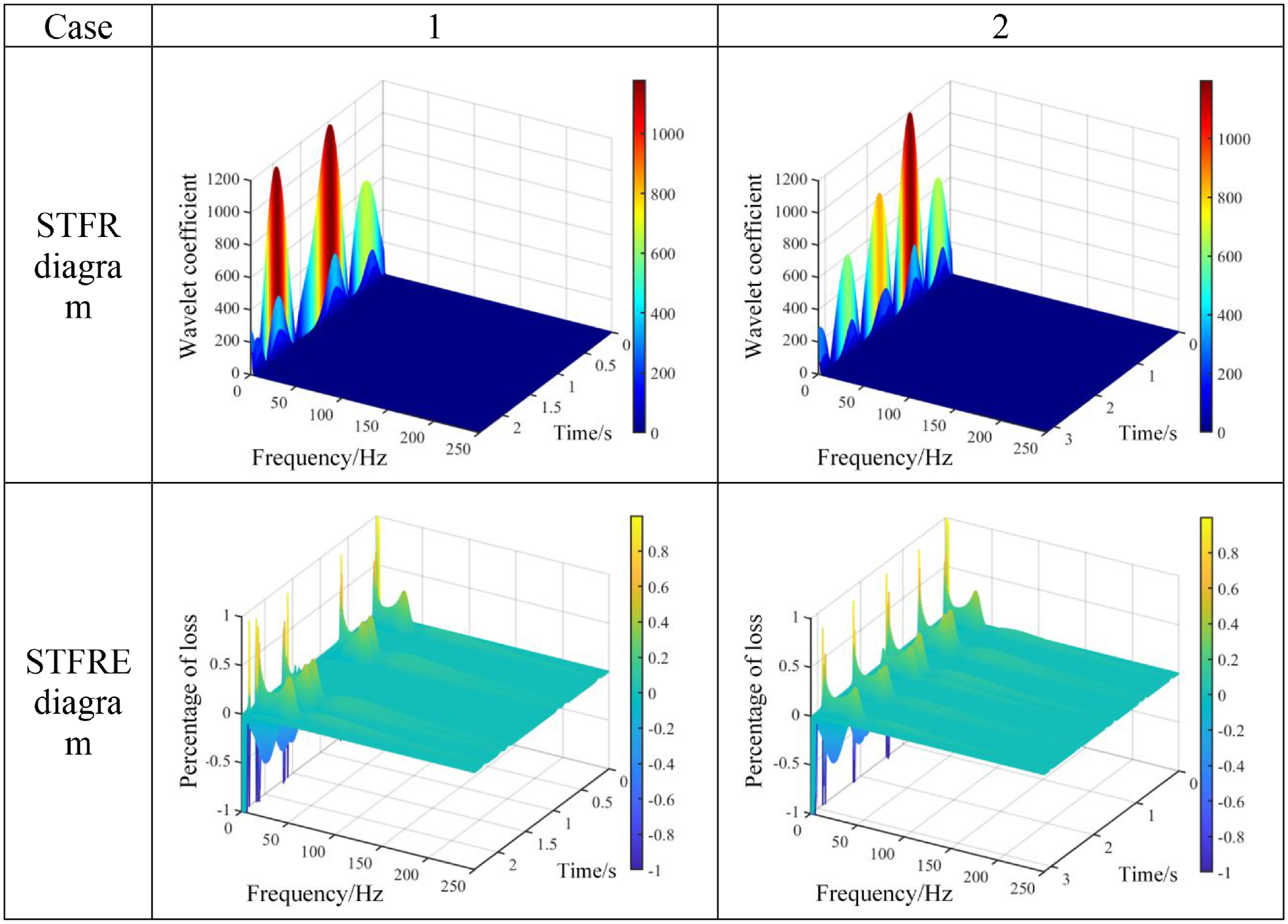
The STFR diagram and STFRE diagram of the two cases.
Theoretical significance and application prospects of SLET
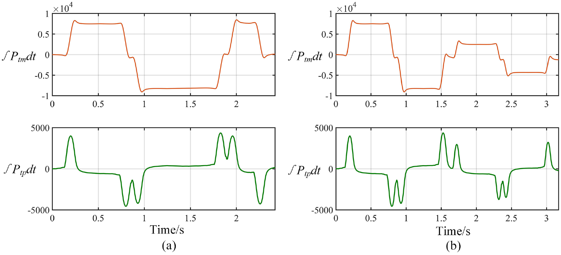
The tracking error is the result of the simultaneous action of amplitude attenuation and phase lag of the servo system, which cannot be distinguished only by traditional methods such as time-domain comparison or frequency-domain FFT analysis. The solution method of SLET can separate the effects of amplitude attenuation and phase lag on the setpoints.
As shown in Figure 11,
Theoretical significance and application prospect of SLEF
Generally, the frequency component loss of an input signal passing through the servo control system can be characterized by the difference between the input and output Fourier transform. This method is actually equivalent to making the signal pass through a system with zero phase lag, only considering the effect of the amplitude frequency characteristics, but losing the action process of phase lag. It is obvious that the calculation method of frequency component loss based on Fourier transform is deficient. The SLEF proposed is helpful to explore the relationship between the SL in the frequency-domain and the tracking error.
According to the method described in Section5.3, the SLEF
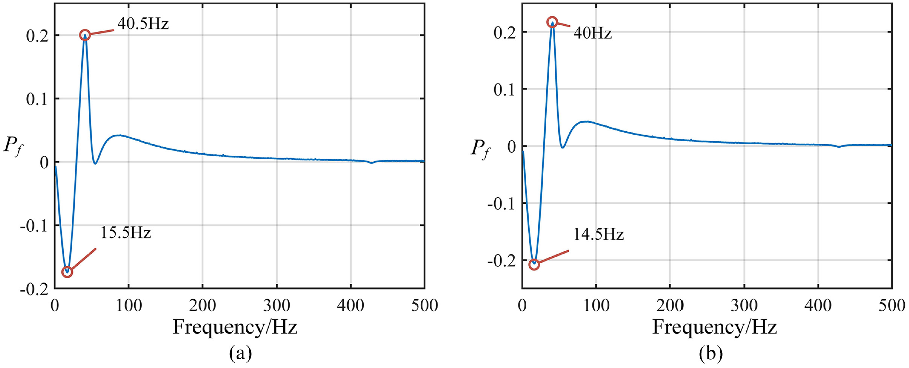
The SLEF of the two cases: (a) Case 1 and (b) Case 2.
It can be seen from Figure 13 that the dominant SL occurs near 15 and 40 Hz. It means the servo control system has insufficient performance near the frequency points, meanwhile the setpoints energy is concentrated around the frequency points.
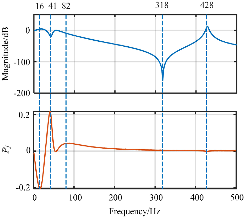
Compared with the amplitude-frequency characteristics of Bode diagram,
Comparison between
Adding filter controller is a common method to improve the servo bandwidth and to reduce the tracking error. Usually, the frequency band of the filter should be judged by amplitude-frequency characteristic of the servo control system. As shown in Figure 14, only from the perspective of the amplitude-frequency characteristics, the frequency bands near 16, 41, 318, and 428 Hz may be the dominant frequency band that should be filtered. However, if the
A high-precision servo control system should produce the minimum distortion of the input. Considering the impossibility of the ideal filter, the spectrum of the real filter cannot be completely box shaped, and the unnecessary addition of filter may deteriorate the system performance.
Solving process
In order to clearly present the computational flow of the proposed method, the solution flow of STFR and STFRE are plotted as shown in Figure 15.
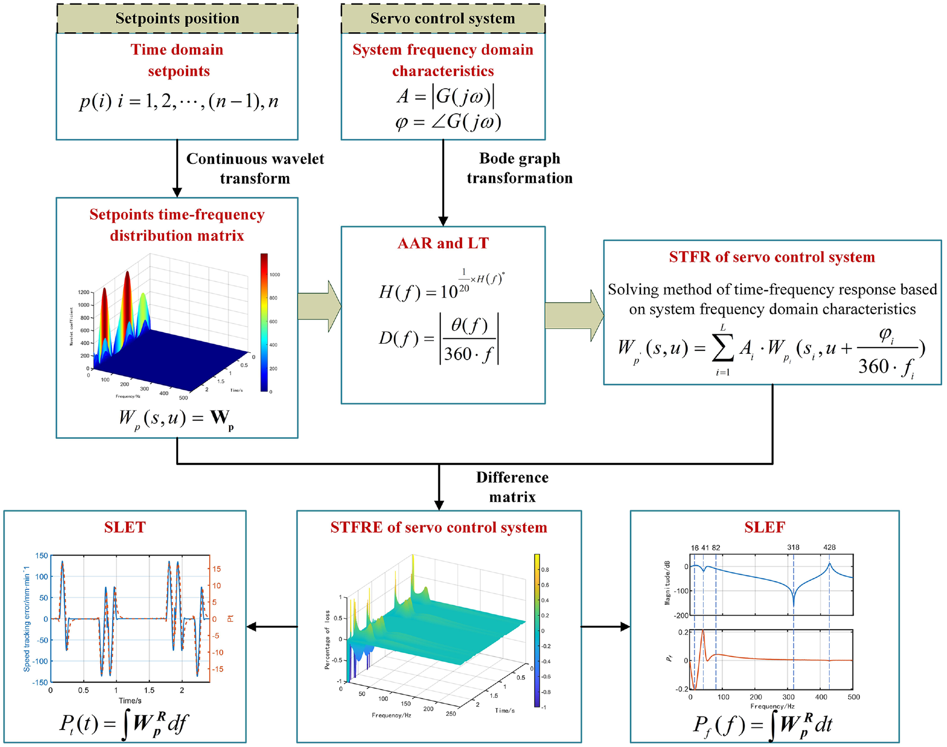
The solving process.
Conclusions
In this paper, a method for solving STFR and STFRE based on the frequency domain characteristics of servo control systems is proposed, which can be used for the analysis of the time-frequency response process of actual motion setpoints.
(1) First, the setpoint is transformed from the time domain to the time-frequency domain by CWT; Then, the AAR expression and LT expression are constructed of the servo control system based on the amplitude-frequency characteristics and phase-frequency characteristics; Finally, the STFR is solved by applying amplitude attenuation and time lag to each frequency component of the setpoints at each moment.
(2) The STFRE including SL, SLET and SLEF are constructed. The former is the ratio of the difference between the setpoints time-frequency matrix and the response time-frequency matrix to the setpoints time-frequency matrix, which represents the loss of each frequency component of the setpoints at each time; The latter two are the integration of SL to frequency and time respectively, representing the setpoints loss at each time and the contribution of each frequency loss to the global loss.
The theoretical significance and application prospects of the present method were found by solving the time-frequency response of two sets of real setpoints:
(1) Compared with the existing analysis methods, the proposed method is not limited to the type of wavelet basis functions and can be applied to the solution of arbitrary STFR.
(2) The time-frequency response solution method is based on the amplitude decay and phase lag of the servo system to the setpoints and is able to separate the SL or tracking error caused by both, and analyze the cause of the tracking error in depth.
(3) The solving method of STFR can determine the redundancy and deficiency of filter and other strategies for a setpoints and servo control system.
The proposed method introduces the adjustment coefficients
Footnotes
Appendix
Declaration of conflicting interests
The author(s) declared no potential conflicts of interest with respect to the research, authorship, and/or publication of this article.
Funding
The author(s) disclosed receipt of the following financial support for the research, authorship, and/or publication of this article: This work is financially supported by the project of National Natural Science Funds of China (Grant No. 52175483, 51775421).