The role of elasticity measures for characterizing anchor points in DEA

Abstract

As an important concept in data envelopment analysis (DEA), elasticity measure has wide theoretical and practical applications in formulating various economic concepts. Anchor points also appear to be particularly interesting and highly useful in DEA, especially for recognizing a decision making unit (DMU) as a benchmark. This paper is an attempt to use left-and right-hand elasticity measures to present a novel definition (characterization) for anchor points. The study results reveal that if there exists an increase in a bundle of input with no rate of change in a bundle of output or if there is a decrease in a bundle of output, but a bundle of input has no rate of change, then such an extreme point is the anchor point.

Introduction

DEA is a useful method to empirically measure peer DMUs productive efficiency with multiple inputs and outputs (see Cooper et al. ¹ ). There are two main types of DEA technologies: constant returns to scale and variable returns to scale, each one creating its own models for evaluation of efficiency. Yu et al. ² provided a different types of extended DEA models. We can impose weight restrictions to incorporate different types of point of views in DEA models (see Allen et al. ³ ). Also, various types of economic concepts may be provided by DEA models (see Ouellette and Vierstraete ⁴ ).

In the meantime, elasticity measures evaluate the responsiveness to a change. Different types of scale elasticity can be seen in Podinovski et al., ⁵ in which the authors presented a simpler formula for calculating scale elasticity than the existed approaches before and utilized the concept of directional derivatives for their development. The concept of elasticity measures and application of directional derivatives can be seen in Podinovski and Førsund, ⁶ in which the theorem of the directional derivative of the optimal value function is used to define and calculate the elasticity measures to the entire efficient frontier. Atici and Podinovski ⁷ investigated various types of elasticity measures with partial orientation. Also, Podinovski et al. ⁸  presented the application of linear programing for calculation of various concepts such as marginal rates, scale elasticity and mixed elasticity measures.

The concept of anchor points can be found in Allen and Thanassoulis. ⁹ Bougnol and Dulá ¹⁰ presented a sufficiently interesting method by considering the geometry of anchor points. Bougnol and Dulá ¹⁰ explored the role of anchor points in the geometry of the DEA production possibility set and showed that anchor points play a major role in defining the shape of production possibility set. Thanassoulis et al.^11,12 introduced a sophisticated approach based on super efficiency to obtain anchor points in VRS technology. Hosseinzadeh Lotfi et al. ¹³ provided a useful algorithm to identify anchor points. The usefulness of sensitivity analysis to obtain anchor points can be seen in Mostafaee and Soleimani-damaneh. ¹⁴ Also, a novel method for obtaining anchor points in FDH models is presented in Soleimani-damaneh and Mostafaee. ¹⁵ Different characterizations of anchor points may be obtained in Mostafaee and Soleimani-Damaneh. ¹⁶ Also, Edvardsen et al. ¹⁷ determined exterior points by a different point of view. The concept of terminal points can be seen in Krivonozhko et al. ¹⁸ There are various kinds of relationships between different subsets of extreme points (see Charnes et al. ¹⁹ and Krivonozhko et al. ²⁰ ). Different characterizations of terminal, anchor and exterior points in DEA are also presented in Mostafaee and Sohraiee. ²¹

This paper presents a novel definition (characterization) for recognizing anchor points in variable returns to scale (VRS) technology. In particular, we utilize the concept of left- and right-hand elasticity measures to obtain a distinctive outlook for anchor points.

The paper includes five sections: After the Introduction Section, the Preliminaries is presented in Section 2. We can see the proposed definition of anchor points and the theorems which have been proved in Section 3. We illustrate the new definition of anchor points together with a detailed description of some examples in Section 3. The conclusion of the paper is provided in Section 4.

Preliminaries

Suppose that we have a set of n observed production units $(X_j,Y_j),j=1,\dots n$ , where non-zero inputs $X_j=(x_{1j},\dots ,x_{\mathrm{mj}})\ge 0$ produce non-zero outputs $Y_j=(y_{1j},\dots ,y_{\mathrm{sj}})\ge 0$ . We express each production unit as follows (Transpose is denoted by superscript “t”):

$$\mathrm{DM}{U}_j=(X_j,Y_j{)}^t,j=1,\dots ,n$$

(1)

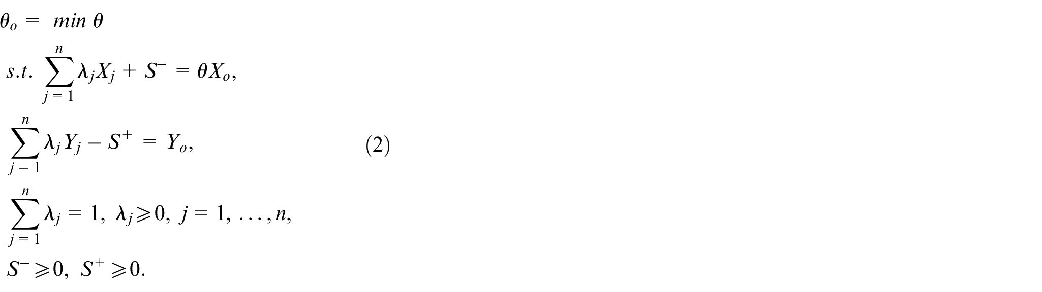
The BCC efficiency model of $\mathrm{DM}{U}_0=(X_o,Y_o{)}^t(1\le o\le n)$ in its input orientation is (see Banker et al. ²² ):

$$\begin{array}{c}{\theta }_o=\min \theta \hfill \\ s.t.\sum _{j=1}^n{\lambda }_j{X}_j+S^{-}=\theta X_o,\hfill \\ \sum _{j=1}^n{\lambda }_j{Y}_j-S^{+}=Y_o,\hfill \\ \sum _{j=1}^n{\lambda }_j=1,{\lambda }_j\ge 0,j=1,\dots ,n,\hfill \\ S^{-}\ge 0,S^{+}\ge 0.\hfill \end{array}$$

(2)

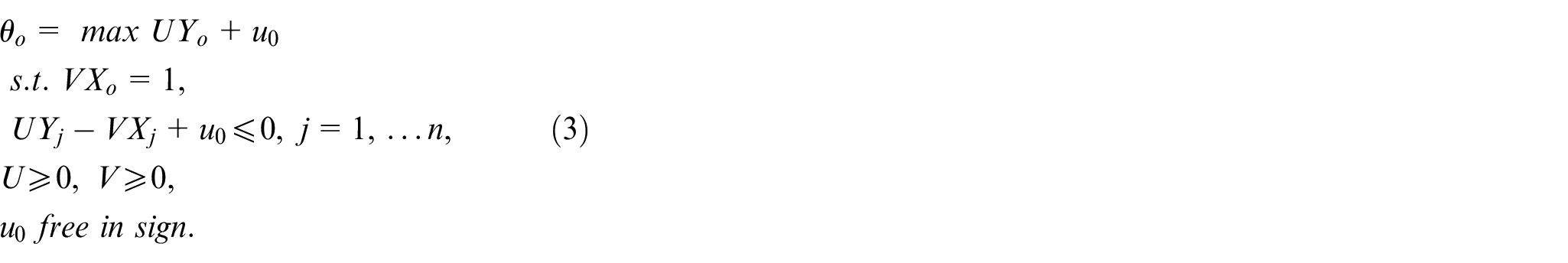
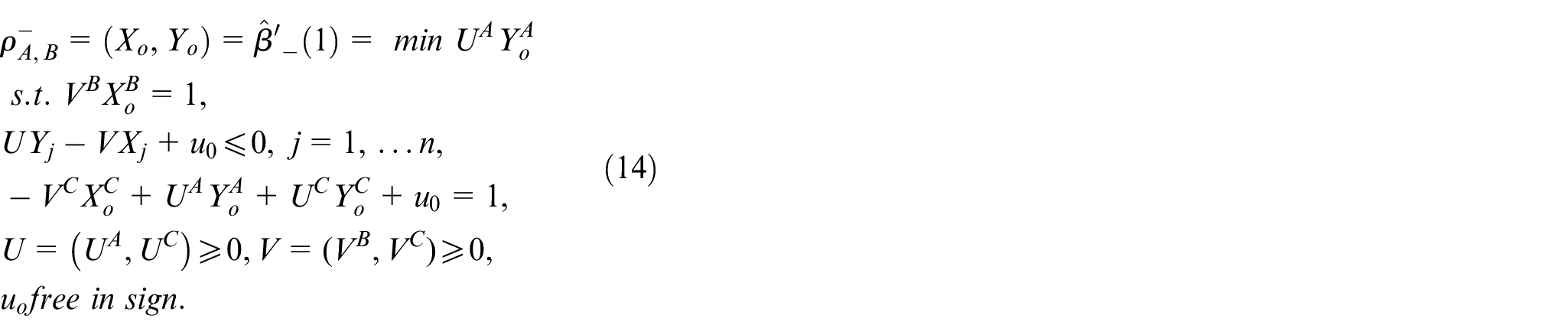
The dual problem of Model (2) may be represented as follows:

$$\begin{array}{c}{\theta }_o=\max U{Y}_o+u_0\hfill \\ s.t.V{X}_o=1,\hfill \\ U{Y}_j-V{X}_j+u_0\le 0,j=1,\dots n,\hfill \\ U\ge 0,V\ge 0,\hfill \\ u_0\mathrm{free}\mathrm{in}\mathrm{sign}.\hfill \end{array}$$

(3)

The BCC efficiency of $\mathrm{DM}{U}_0=(X_o,Y_o{)}^t(1\le o\le n)$ in its input orientation is achieved, if ${\theta }_o=1$ and all slacks $S^{-}=0$ and $S^{+}=0$ in all optimal solutions of Model (2).

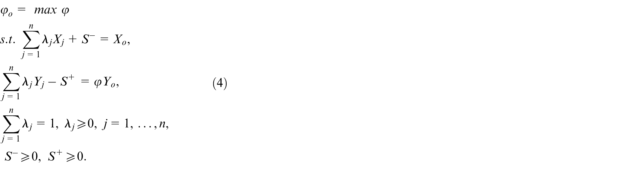
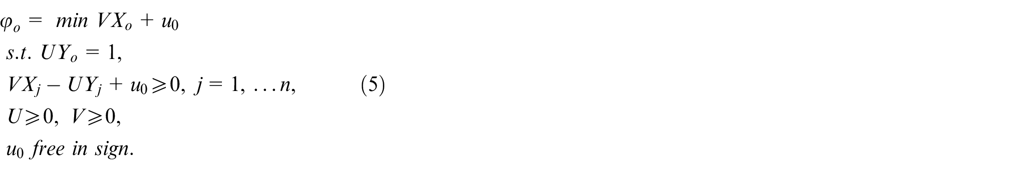
The BCC efficiency models of $\mathrm{DM}{U}_0=(X_o,Y_o{)}^t(1\le o\le n)$ in output orientation are as follows:

$$\begin{array}{c}{\phi }_o=\max \phi \hfill \\ s.t.\sum _{j=1}^n{\lambda }_j{X}_j+S^{-}=X_o,\hfill \\ \sum _{j=1}^n{\lambda }_j{Y}_j-S^{+}=\phi Y_o,\hfill \\ \sum _{j=1}^n{\lambda }_j=1,{\lambda }_j\ge 0,j=1,\dots ,n,\hfill \\ S^{-}\ge 0,S^{+}\ge 0.\hfill \end{array}$$

(4)

$$\begin{array}{c}{\phi }_o=\min V{X}_o+u_0\hfill \\ s.t.U{Y}_o=1,\hfill \\ V{X}_j-U{Y}_j+u_0\ge 0,j=1,\dots n,\hfill \\ U\ge 0,V\ge 0,\hfill \\ u_0\mathrm{free}\mathrm{in}\mathrm{sign}.\hfill \end{array}$$

(5)

The BCC efficiency of $\mathrm{DM}{U}_0=(X_o,Y_o{)}^t(1\le o\le n)$ in its input orientation is achieved, if ${\phi }_o=1$ and all slacks $S^{-}=0$ and $S^{+}=0$ in all optimal solutions of Model (4).

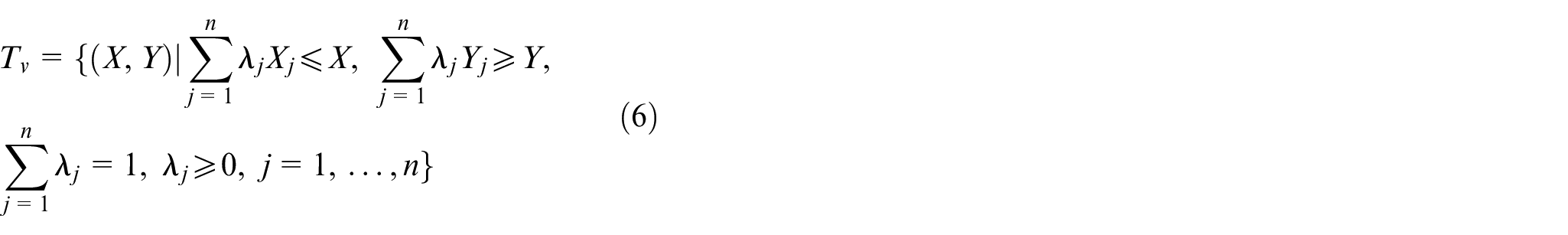
The production possibility set (PPS) $T_v$ with variable returns to scale technology can be expressed as follows:

$$\begin{array}{c}{T}_v=\{(X,Y)|\sum _{j=1}^n{\lambda }_j{X}_j\le X,\sum _{j=1}^n{\lambda }_j{Y}_j\ge Y,\hfill \\ \sum _{j=1}^n{\lambda }_j=1,{\lambda }_j\ge 0,j=1,\dots ,n\}\hfill \end{array}$$

(6)

Regarding $T_v\subset {\mathbb{R}}^{m+s}$ , the hyperplane that supports $T_v$ is as follows:

$$H_{(U,V,u_0)}=\{(X,Y)\in {\mathbb{R}}^{m+s}|\mathrm{UY}-\mathrm{VX}+u_0=0\}.$$

Denote the set of all boundary production units of $T_v$ as $\partial T_v$ . In this paper, the set of indices of all vertex production units is expressed by $E$ (see Bazaraa et al. ²³ and Bazaraa et al. ²⁴ ). Podinovski and Førsund ⁶ proposed three disjoint sets for all inputs and all outputs: $A$ , $B$ and $C$ . Also, they considered the rate of changes of the components that belong to $B$ in relation to changes of the components that belong to $A$ , with the assumption of the unchanged components in $C$ . In this paper, two general scenarios are considered:

• Scenario 1: $A\ne Ø$ with input indices, B≠ with outputs indices and $A\cap B=Ø$ and $C=(A\cup B{)}^c$ “c” stands for complement.

• Scenario 2: $A\ne Ø$ with output indices, $B\ne Ø$ with input indices and $A\cap B=Ø$ and $C=(A\cup B{)}^c$ , “c” stands for complement.

• Scenario 1: In this case, each $\mathrm{DM}{U}_o=(X_o,Y_o{)}^t\in T_v$ can be represented as $\mathrm{DM}{U}_o=(X_o^A,X_o^C,Y_o^B,Y_o^C{)}^t$ in which vectors $X_o^A$ and $X_o^C$ are the components of vector of input $X_o$ that their indices belong to the sets $A$ and $C$ , respectively and vectors $Y_o^B$ and $Y_o^C$ are the components of vector of output $Y_o$ that their indices belong to the sets $B$ and $C$ , respectively. Assuming that $X_o^A>0$ and $Y_o^B$ has at least one positive component, the function that shows the response of outputs can be expressed as follows:

$$\overline{\beta }\left(\alpha \right)=\max \left\{\beta |{(\alpha X_o^A,X_o^C,\beta Y_o^B,Y_o^C)}^tϵT_v\right\}$$

(7)

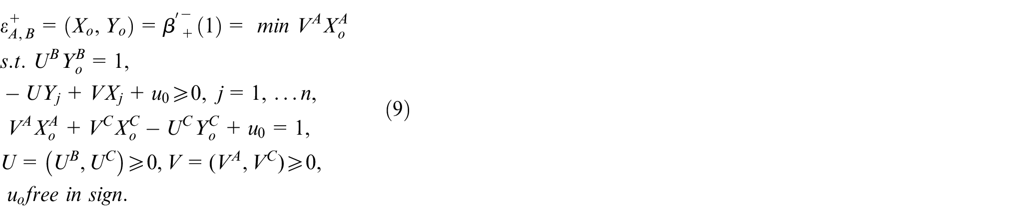
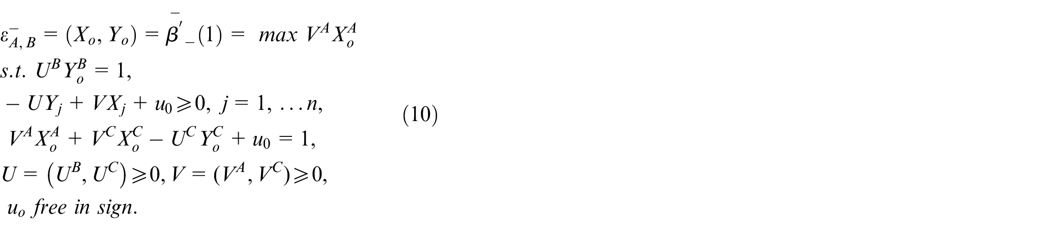
• Definition 2.1 (see Podinovski and Førsund  ⁶ ) With the differentiability assumption of $\overline{\beta }(\alpha )$ at $\alpha =1$ , the elasticity of change of set of output $Y_o^B$ with respect to set of input $X_o^A$ is as follows:

$${ϵ}_{A,B}(X_o,Y_o)=\stackrel{-}{{\beta }^{\prime }}\left(1\right).$$

(8)

• Theorem 2.2 (see Podinovski and Førsund  ⁶ )

• (a) Assume that the function $\overline{\beta }(\alpha )$ has been defined in some right (left) neighborhood of $\alpha =1$ . This implies a finite right-hand (respectively, left-hand) derivative as follows:

$$\begin{array}{c}{\epsilon }_{A,B}^{+}=(X_o,Y_o)={{\beta }^{\prime }}_{+}^{-}\left(1\right)=\min V^A{X}_o^A\hfill \\ s.t.U^B{Y}_o^B=1,\hfill \\ -U{Y}_j+V{X}_j+u_0\ge 0,j=1,\dots n,\hfill \\ V^A{X}_o^A+V^C{X}_o^C-U^C{Y}_o^C+u_0=1,\hfill \\ U=(U^B,U^C)\ge 0,V=(V^A,V^C)\ge 0,\hfill \\ u_o\mathrm{free}\mathrm{in}\mathrm{sign}.\hfill \end{array}$$

(9)

and,

$$\begin{array}{c}{\epsilon }_{A,B}^{-}=(X_o,Y_o)={\stackrel{-}{{\beta }^{\prime }}}_{-}\left(1\right)=\max V^A{X}_o^A\hfill \\ s.t.U^B{Y}_o^B=1,\hfill \\ -U{Y}_j+V{X}_j+u_0\ge 0,j=1,\dots n,\hfill \\ V^A{X}_o^A+V^C{X}_o^C-U^C{Y}_o^C+u_0=1,\hfill \\ U=(U^B,U^C)\ge 0,V=(V^A,V^C)\ge 0,\hfill \\ u_o\mathrm{free}\mathrm{in}\mathrm{sign}.\hfill \end{array}$$

(10)

in which weight vectors $V^A$ and $V^C$ are the components of weight vector of input $V$ that belong to the sets $A$ and $C$ , respectively and weight vectors $U^B$ and $U^c$ are the components of weight vector of output U that belong to the sets $B$ and $C$ , respectively.

• (b) Assume that $\overline{\beta }(\alpha )$ is undefined in the right (left) of $\alpha =1$ . This implies the unboundedness of objective function of Model (9) (Model (10)).

The left- and right-hand elasticity measures for output sets can be obtained by Models (9) and (10), respectively.

Scenario 2: In this case, each $\mathrm{DM}{U}_o=(X_o,Y_o{)}^t\in T_v$ can be represented as $\mathrm{DM}{U}_o=(X_o^B,X_o^C,Y_o^A,Y_o^C{)}^t$ in which vectors of input $X_o^B$ and $X_o^C$ are the components that their indices belong to the sets $B$ and $C$ , respectively and also, vectors of output $Y_o^A$ and $Y_o^C$ are the components that their indices belong to the sets $A$ and $C$ , respectively. Suppose that $Y_o^A>0$ and $X_o^B$ has at least one positive component. Thus, the function that shows the response of inputs can be expressed as follows:

$$\hat{\beta }\left(\alpha \right)=\min \left\{\beta |{(\beta X_o^B,X_o^C,\alpha Y_o^A,Y_o^C)}^tϵT_v\right\}$$

(11)

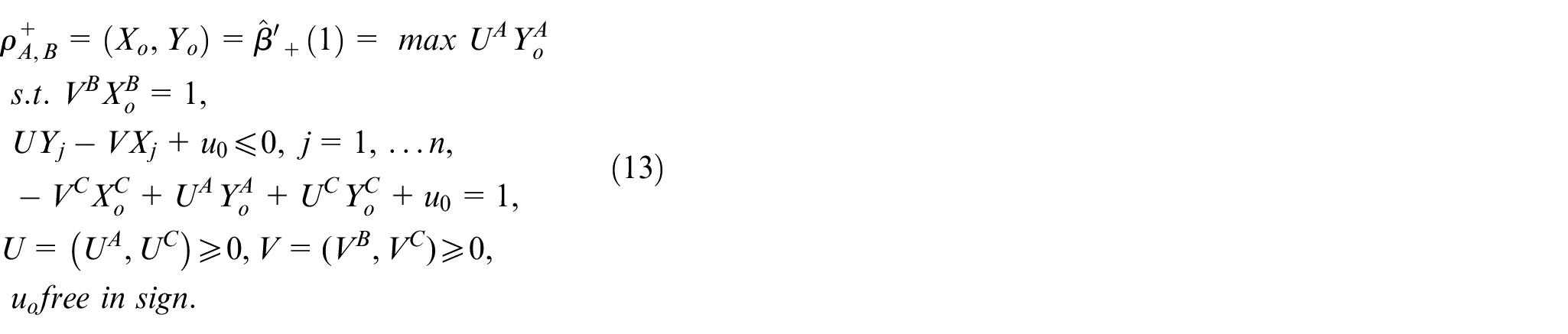
• Definition 2.3 (see Podinovski and Førsund ⁶ ) With the differentiability assumption of $\hat{\beta }(\alpha )$ at $\alpha =1$ , the elasticity of change of set of input $X_o^B$ with respect to set of output $Y_o^A$ is as follows:

$${\rho }_{A,B}(X_o,Y_o)=\hat{\beta }\prime \left(1\right).$$

(12)

• Theorem 2.4 (see Podinovski and Førsund ⁶ )

• (a) Assume that the function $\hat{\beta }(\alpha )$ has been defined in some right (left) neighborhood of $\alpha =1$ . This implies a finite right-hand (respectively, left-hand) derivative as follows:

$$\begin{array}{c}{\rho }_{A,B}^{+}=(X_o,Y_o)={\hat{\beta }\prime }_{+}\left(1\right)=\max U^A{Y}_o^A\hfill \\ s.t.V^B{X}_o^B=1,\hfill \\ U{Y}_j-V{X}_j+u_0\le 0,j=1,\dots n,\hfill \\ -V^C{X}_o^C+U^A{Y}_o^A+U^C{Y}_o^C+u_0=1,\hfill \\ U=(U^A,U^C)\ge 0,V=(V^B,V^C)\ge 0,\hfill \\ u_o\mathrm{free}\mathrm{in}\mathrm{sign}.\hfill \end{array}$$

(13)

and,

$$\begin{array}{c}{\rho }_{A,B}^{-}=(X_o,Y_o)={\hat{\beta }\prime }_{-}\left(1\right)=\min U^A{Y}_o^A\hfill \\ s.t.V^B{X}_o^B=1,\hfill \\ U{Y}_j-V{X}_j+u_0\le 0,j=1,\dots n,\hfill \\ -V^C{X}_o^C+U^A{Y}_o^A+U^C{Y}_o^C+u_0=1,\hfill \\ U=(U^A,U^C)\ge 0,V=(V^B,V^C)\ge 0,\hfill \\ u_o\mathrm{free}\mathrm{in}\mathrm{sign}.\hfill \end{array}$$

(14)

in which weight vectors $V^B$ and $V^C$ are the components of weight vector of input $V$ that belong to the sets $B$ and $C$ , respectively and weight vectors $U^A$ and $U^c$ are the components of weight vector of output U that belong to the sets $A$ and $C$ , respectively.

• (b) Assume that $\hat{\beta }(\alpha )$ is undefined in the right (left) of $\alpha =1$ . This implies the unboundedness of objective function of Model (13) (Model (14)).

The left- and right-hand elasticity measures for input sets can be achieved by Models (13) and (14), respectively.

• Definition 2.5 (see Bougnol and Dulá ¹⁰ and Mostafaee and Soleimani-Damaneh ¹⁶ ). $\mathrm{DM}{U}_o,o\in E$ can be considered as anchor if and only if there exist a hyperplane

$$H_{(U,V,u_0)}=\{(X,Y)\in {\mathbb{R}}^{m+s}|\mathrm{UY}-\mathrm{VX}+u_0=0\}.$$

Such that supports $T_v$ at $\mathrm{DM}{U}_o$ , and there exists at least one $1\le r\le s$ for which $u_r$ is zero or at least one $1\le i\le m$ for which $v_i$ is zero.

Main results

In this section, a new characterization of anchor points that may be considered as a novel definition, is presented. We show the equivalency of both definitions in a theorem. Also, the truthfulness of theorem is illustrated by two examples.

• Definition 3.1 $\mathrm{DM}{U}_o=(X_o,Y_o{)}^t,o\in E$ can be considered as anchor, if at least one of the following conditions are satisfied:

• (a) There exists an output bundle $Y_o^{\overline{B}}$ with respect to the input bundle $X_o^{\overline{A}}$ such that ${\epsilon }_{\overline{A},\overline{B}}^{+}(X_o,Y_o)={{\overline{\beta }}^{\prime }}_{+}\left(1\right)=0.$

• (b) There exists an input bundle $X_o^{\hat{B}}$ with respect to the output bundle $Y_o^{\hat{A}}$ such that ${\rho }_{\hat{A},\hat{B}}^{-}(X_o,Y_o)={\hat{\beta }\prime }_{-}\left(1\right)=0.$

• Theorem 3.2 Definitions 2.5 and 3.1 are equivalent.

Proof. Suppose that Definition 3.1 is held by $\mathrm{DM}{U}_o\in E$ . Thus, there exists an output bundle $Y_o^{\overline{B}}$ with respect to the input bundle $X_o^{\overline{A}}$ such that ${\epsilon }_{\overline{A},\overline{B}}^{+}(X_o,Y_o)=\underset{+}{{\overline{\beta }}^{\prime }}\left(1\right)=0$ , or there exists an input bundle $X_o^{\hat{B}}$ with respect to the output bundle $Y_o^{\hat{A}}$ such that ${\rho }_{\hat{A},\hat{B}}^{-}(X_o,Y_o)={\hat{\beta }\prime }_{-}\left(1\right)=0$ . To continue, first, suppose that ${\epsilon }_{\overline{A},\overline{B}}^{+}(X_o,Y_o)=\underset{+}{{\overline{\beta }}^{\prime }}\left(1\right)=0$ . Therefore, Model (9) has a zero optimal solution. Suppose $(U^{*},V^{*},u_0^{*})$ satisfies the optimality conditions of Model (9). Since, $V^{*\overline{A}}{X}_o^{\overline{A}}=0,V^{*\overline{A}}\ge 0$ and $X_o^{\overline{A}}>0$ we have

$$V^{*\overline{A}}=0$$

(15)

Also, the second and third constraints of Model (9), implies that

$$-U^{*}{Y}_o+V^{*}{X}_o+u_0^{*}=0$$

(16)

By setting $U^{*\overline{B}}{Y}_o^{\overline{B}}+U^{*\overline{C}}{Y}_o^{\overline{C}}=U^{*}{Y}_o=\alpha \ge 1$ two possible cases can be considered:

• (a) If $\alpha =1$ then $(U^{*},V^{*},u_0^{*})$ is feasible for Model (5) and $V^{*}{X}_o+u_0^{*}=U^{*}{Y}_o=1$ . This implies the optimality of $(U^{*},V^{*},u_0^{*})$ for Model (5). Thus

$$H_{(U^{*},V^{*},u_0^{*})}=\{(X,Y)\in {\mathbb{R}}^{m+s}|-U^{*}Y+V^{*}X+u_0^{*}=0\}$$

Supports $T_v$ at $\mathrm{DM}{U}_o$ , and by (15), $v_i^{*}=0$ for $i\in \overline{A}$ . Hence, $\mathrm{DM}{U}_o$ can be considered as anchor by Definition 2.5.

• (b) If $\alpha >1$ then obviously $(\frac{U^{*}}{\alpha },\frac{V^{*}}{\alpha },\frac{u_0^{*}}{\alpha })$ is feasible for Model (5) and also $\frac{V^{*}}{\alpha }{X}_o+\frac{u_0^{*}}{\alpha }=\frac{U^{*}}{\alpha }{Y}_0=1$ . This implies the optimality of $(\frac{U^{*}}{\alpha },\frac{V^{*}}{\alpha },\frac{u_0^{*}}{\alpha })$ for Model (5). It means

$$H_{({\frac{U}{\alpha }}^{*},{\frac{V}{\alpha }}^{*},\frac{u_0^{*}}{\alpha })}=\{(X,Y)\in {\mathbb{R}}^{m+s}|-{\frac{U}{\alpha }}^{*}Y+{\frac{V}{\alpha }}^{*}X+\frac{u_0^{*}}{\alpha }=0\}$$

Supports $T_v$ at $\mathrm{DM}{U}_o$ , and by (15), $\frac{v_i^{*}}{\alpha }=0$ for $i\in \overline{A}$ . Thus, $\mathrm{DM}{U}_o$ is anchor by Definition 2.5.

To complete the proof of if part, suppose that there exists an input bundle $X_o^{\hat{B}}$ with respect to the output bundle $Y_o^{\hat{A}}$ such that ${\rho }_{\hat{A},\hat{B}}^{-}(X_o,Y_o)=\underset{-}{\hat{\beta }\prime }\left(1\right)=0$ . Therefore, Model (14) has zero as optimal solution. Consider $(U^{*},V^{*},u_0^{*})$ as optimal solution of Model (14). Since, $U^{*\hat{A}}{Y}_o^{\hat{A}}=0,U^{*\hat{A}}\ge 0$ and $Y_o^{\hat{A}}>0$ we have

$$U^{*\hat{A}}=0$$

(17)

Also, second and third constraints of Model (14) implies,

$$U^{*}{Y}_o-V^{*}{X}_o+u_0^{*}=0$$

(18)

By setting $V^{*\hat{B}}{X}_o^{\hat{B}}+V^{*\hat{C}}{X}_o^{\hat{C}}=V^{*}{X}_o=\beta \ge 1$ , we can consider two possible cases two possible cases:

• (c) If $\beta =1$ then Model (3) is feasible at $(U^{*},V^{*},u_0^{*})$ , and $V^{*}{X}_o=u_0^{*}+U^{*}{Y}_o=1$ . It means the optimality of $(U^{*},V^{*},u_0^{*})$ for Model (3). Thus

$$H_{(U^{*},V^{*},u_0^{*})}=\{(X,Y)\in {\mathbb{R}}^{m+s}|U^{*}Y-V^{*}X+u_0^{*}=0\}$$

Supports $T_v$ at $\mathrm{DM}{U}_o$ , and by (17), $u_k^{*}=0$ for $k\in \hat{A}$ . Hence, $\mathrm{DM}{U}_o$ is anchor by Definition 2.5.

• (d) If $\beta >1$ then feasibility of $(\frac{U^{*}}{\beta },\frac{V^{*}}{\beta },\frac{u_0^{*}}{\beta })$ is obvious for Model (3) and also $\frac{V^{*}}{\beta }{X}_o=\frac{u_0^{*}}{\beta }+\frac{U^{*}}{\beta }{Y}_0=1$ . Thus, optimality of $(\frac{U^{*}}{\beta },\frac{V^{*}}{\beta },\frac{u_0^{*}}{\beta })$ is trivial for Model (3). This implies that there exists a hyperplane

$$H_{({\frac{U}{\beta }}^{*},{\frac{V}{\beta }}^{*},\frac{u_0^{*}}{\beta })}=\{(X,Y)\in {\mathbb{R}}^{m+s}|{\frac{U}{\beta }}^{*}Y-{\frac{V}{\beta }}^{*}X+\frac{u_0^{*}}{\beta }=0\}$$

Such that supports $T_v$ at $\mathrm{DM}{U}_o$ , and by (17), $\frac{u_k^{*}}{\beta }=0$ for k $\in \hat{A}$ . Thus, $\mathrm{DM}{U}_o$ is anchor by Definition 2.5. the half of proof has been done.

Conversely, suppose that $\mathrm{DM}{U}_o,o\in E$ is anchor by Definition 2.5. Thus, there exists a hyperplane

$$H_{(\tilde{U},\tilde{V},{\tilde{u}}_0)}=\{(X,Y)\in {\mathbb{R}}^{m+s}|\tilde{V}X-\tilde{U}Y+{\tilde{u}}_0=0\}$$

Such that supports $T_v$ at $\mathrm{DM}{U}_o$ , and there exists $1\le r\le s$ for which ${\tilde{U}}_r$ is zero or there exists $1\le i\le m$ for which ${\tilde{V}}_i$ is zero. Without loss of generality, suppose that ${\tilde{V}}_t=0$ for $t\in \tilde{A}$ such that $1\le \left|\tilde{A}\right|\le m$ or ${\tilde{U}}_r=0$ for $r\in \tilde{A}$ such that $1\le \left|\tilde{A}\right|\le s$ (It is obvious that at least one must be non-zero). If ${\tilde{V}}_t=0$ for $t\in \tilde{A}$ such that $1\le \left|\tilde{A}\right|\le m$ then

$$\tilde{V}{X}_o-\tilde{U}{Y}_o+{\tilde{U}}_0=0$$

(19)

And

$$\tilde{V}{X}_j-\tilde{U}{Y}_j+{\tilde{U}}_0\le 0,\forall j$$

(20)

By letting,

$$\tilde{U}{Y}_o=\gamma >0$$

(21)

We get,

$$\tilde{V}{X}_o+{\tilde{U}}_0=\gamma$$

(22)

Denoting $\frac{\tilde{U}}{\gamma },\frac{\tilde{V}}{\gamma }$ and $\frac{{\tilde{U}}_0}{\gamma }$ by $\tilde{U},\tilde{V}$ and ${\tilde{U}}_0$ , respectively, and dividing the constraints (19), (20), (21), and (22) by $\gamma$ , we get

$$\tilde{V}{X}_o-\tilde{U}{Y}_o+{\tilde{U}}_0=0$$

(23)

$$\tilde{V}{X}_j-\tilde{U}{Y}_j+{\tilde{U}}_0\le 0,\forall j$$

(24)

$$\tilde{U}{Y}_o=1,$$

(25)

And,

$$\tilde{V}{X}_o+{\tilde{U}}_0=1$$

(26)

By (23) and (25), we have

$$-{\tilde{U}}^{\tilde{B}}{Y}_o^{\tilde{B}}-{\tilde{U}}^{\tilde{C}}{Y}_o^{\tilde{C}}+{\tilde{V}}^{\tilde{A}}{X}_o^{\tilde{A}}+{\tilde{V}}^{\tilde{C}}{X}_o^{\tilde{C}}+{\tilde{u}}_0=0,$$

(27)

$${\tilde{U}}^{\tilde{B}}{Y}_o^{\tilde{B}}+{\tilde{U}}^{\tilde{C}}{Y}_o^{\tilde{C}}=1,$$

(28)

Now, we consider two possible cases:

• (e) If $\stackrel{\tilde{B}}{\tilde{U}}{Y}_o^{\tilde{B}}=1$ then by (28), $\stackrel{\tilde{C}}{\tilde{U}}{Y}_o^{\tilde{C}}=0$ and by (27), $-\stackrel{\tilde{B}}{\tilde{U}}{Y}_o^{\tilde{B}}+\stackrel{\tilde{A}}{\tilde{V}}{X}_o^{\tilde{A}}+\stackrel{\tilde{C}}{\tilde{V}}{X}_o^{\tilde{C}}+\underset{0}{\tilde{u}}=0$ .

It follows that, $\stackrel{\tilde{A}}{\tilde{V}}{X}_o^{\tilde{A}}+\stackrel{\tilde{C}}{\tilde{V}}{X}_o^{\tilde{C}}+\underset{0}{\tilde{u}}=1$ . Thus, the feasibility of $(\tilde{U},\tilde{V},{\tilde{u}}_0)$ for Model (9) is obvious and since, $\underset{t}{\tilde{V}}=0$ for $t\in \tilde{A}$ and $\stackrel{\tilde{A}}{\tilde{V}}{X}_o^{\tilde{A}}\ge 0$ , hence, optimality of $(\tilde{U},\tilde{V},{\tilde{U}}_0)$ for Model (9) is attained with zero optimal value. It means that ${\epsilon }_{\tilde{A},\tilde{B}}^{+}(X_o,Y_o)=0$ .

• (f) If $\stackrel{\tilde{B}}{\tilde{U}}{Y}_o^{\tilde{B}}=\delta <1$ then $\frac{{\tilde{U}}^{\tilde{B}}}{\delta }{Y}_o^{\tilde{B}}=1$ . Also, by (27), we get $\frac{1}{\delta }(-\stackrel{\tilde{B}}{\tilde{U}}{Y}_o^{\tilde{B}}-\stackrel{\tilde{C}}{\tilde{U}}{Y}_o^{\tilde{C}}+\stackrel{\tilde{A}}{\tilde{V}}{X}_o^{\tilde{A}}+\stackrel{\tilde{C}}{\tilde{V}}{X}_o^{\tilde{C}}+\underset{0}{\tilde{u}}=0)$ . It means that $-\frac{{\tilde{U}}^{\tilde{C}}}{\delta }{Y}_o^{\tilde{C}}+\frac{{\tilde{V}}^{\tilde{A}}}{\delta }{X}_o^{\tilde{A}}+\frac{{\tilde{V}}^{\tilde{C}}}{\delta }{X}_o^{\tilde{C}}+\frac{{\tilde{u}}_0}{\delta }=1$ . Therefore, $(\frac{\tilde{U}}{\delta },\frac{\tilde{V}}{\delta },\frac{{\tilde{U}}_0}{\delta })$ is optimal for Model (9) with zero as an optimal value. It means that ${\epsilon }_{\tilde{A},\tilde{B}}^{+}(X_o,Y_o)=0$ . The proof of the case $\underset{r}{\tilde{U}}=0$ for some $r=1,\dots ,s$ is similar and is hence omitted. These complete the proof. ■

A special case of Definition 3.1 and Theorem 3.2 can be provided as follows:

• Definition 3.3 $\mathrm{DM}{U}_o=(X_o,Y_o{)}^t,o\in E$ can be considered as anchor, if at least one of the following conditions are satisfied:

• (a) There exists an output $y_{\mathrm{ko}},k=1,\dots ,s$ with respect to the input $x_{\mathrm{to}},t=1,\dots ,m$ such that ${\epsilon }_{t,k}^{+}(X_o,Y_o)=\underset{+}{\overset{-}{{\beta }^{\prime }}}\left(1\right)=0.$

• (b) There exists an input $x_{\mathrm{lo}},l=1,\dots ,m$ with respect to the output $y_{\mathrm{po}},p=1,\dots ,s$ such that ${\rho }_{p,l}^{-}(X_o,Y_o)={\hat{\beta }\prime }_{-}\left(1\right)=0.$

• Theorem 3.4 Definitions 2.5 and 3.3 are equivalent.

Proof. It is a special case of Theorem 3.2. ■

The following examples illustrate the above-mentioned definitions and theorems.

• Example 3.5 Assume that there are three DMUs each of them uses one input and produces one output as Table 1 .

Table 1.

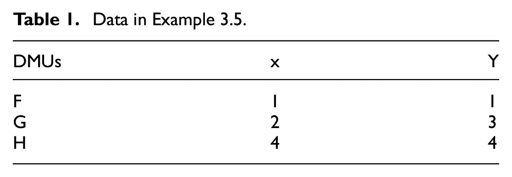
Data in Example 3.5.

DMUs	x	Y
F	1	1
G	2	3
H	4	4

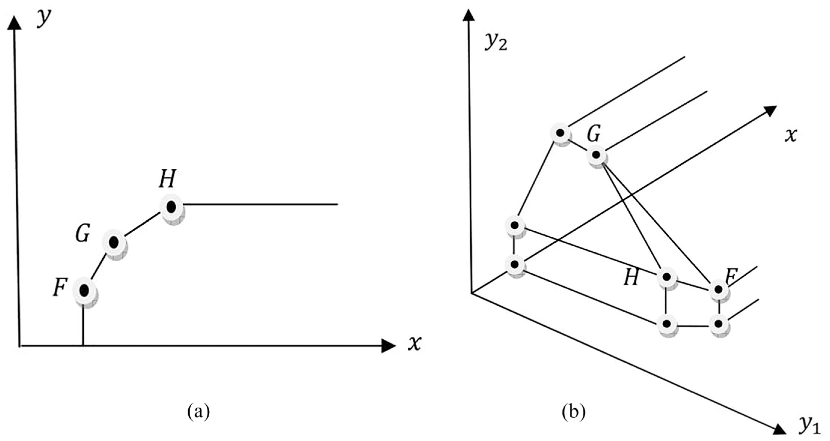
The PPS is depicted in Figure 1(a). By Figure 1(a), DMUs F and H are anchor. Suppose $A=\left\{\mathrm{input}\right\}$ , $B=\left\{\mathrm{output}\right\}$ and $C=Ø$ . By solving Model (9) for unit H, we get ${\epsilon }_{A,B}^{+}(x_H,y_H)=0$ . It shows that unit H is anchor by Definition 3.1 and Definition 3.3. Also, consider the calculation of elasticity response of input with respect to output. Thus, $A=\left\{\mathrm{output}\right\}$ , $B=\left\{\mathrm{input}\right\}$ and $C=Ø$ . By solving Model (14), we get ${\rho }_{A,B}^{-}(x_F,y_F)=0$ . Therefore, unit F is anchor by Definition 3.1and Definition 3.3. Also, if we solve Model (9) and Model (14) for unit G, we will get ${\epsilon }_{A,B}^{+}(x_G,y_G)=0.33$ and ${\rho }_{A,B}^{-}(x_G,y_G)=0.75$ , respectively. It shows that unit G is not anchor. This example illustrates Theorem 3.2 and Theorem 3.4.

• Example 3.6 Assume that there are three DMUs each of them uses one input and produces two outputs as Table 2 .

Figure 1.

PPS of examples: (a) PPS of Example 3.5 and (b) PPS of Example 3.6.

Table 2.

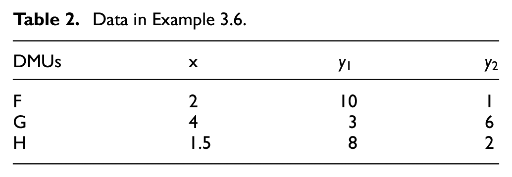
Data in Example 3.6.

DMUs	x	$y_1$	$y_2$
F	2	10	1
G	4	3	6
H	1.5	8	2

The PPS is depicted in Figure 1(b). By Figure 1(b), all three DMUs are anchor. Suppose $A=\left\{\mathrm{input}\right\}$ , $B=\left\{\mathrm{output}2\right\}$ and $C=\left\{\mathrm{output}1\right\}$ . By solving Model (9) for units G and F, we get ${\epsilon }_{A,B}^{+}(x_G,y_G)=0$ and ${\epsilon }_{A,B}^{+}(x_F,y_F)=0$ . It shows that units G and F are anchor units by Definition 3.1 and Definition 3.3. Also, consider the calculation of elasticity response of input with respect to output 2 while keeping output 1 constant. Thus, $A=\left\{\mathrm{output}2\right\}$ , $B=\left\{\mathrm{input}\right\}$ and $C=\left\{\mathrm{output}1\right\}$ . By solving Model (14), we get ${\rho }_{A,B}^{-}(x_H,y_H)=0$ . Therefore, unit F is anchor by Definition 3.1 and Definition 3.3. This example illustrates Theorem 3.2 and Theorem 3.4.

Conclusion

A careful study of elasticity measures made us think about the feasibility of employing left- and right-hand elasticity measures in extreme points to identify anchor points. This attempt led to a new definition in extreme points based on left- and right-hand elasticity measures. The study results demonstrate that the new definition approximates to other previous standard definitions. The paper also aims to present additional characteristics of anchor points. Naturally, the more information we obtain about anchor points, the more deeply we understand their geometry in economics and DEA. When calculating left- and right-hand elasticity measures at extreme points, in addition to economic evidence, one can make use of the provided definition in this paper to identify anchor points, without solving extra anchor point models.