
Abstract
The purpose of this paper is to propose a novel aircraft wing loads calculation model, called long short-term memory residual network (LSTM-ResNet), which can evaluate the loads based on the strain distribution. To achieve this goal, firstly, the data acquisition experiment is designed and performed with a real aircraft wing. In this experiment, we used the Fiber Bragg Grating (FBG) technology as the measurement method to collect strain-load data from the aircraft wing. Then, we propose the LSTM-ResNet model with the one-dimensional convolutional(1D-CNN) architecture. This model is capable of extracting the temporal and spatial representational information from the strain-load data of the aircraft wing. Experimental results demonstrate that the proposed method effectively evaluate the loads of the aircraft wing. To prove the superiority of LSTM-ResNet model, we compared the proposed model with existing loads calculation methods on our experimental dataset. The results show it has a competitive average relative error (0.08%). Moreover, those promising results may pave the way to use the deep learning algorithm in aircraft wing loads calculation.
Introduction
The loads monitoring is an important method of managing the fatigue life of an aircraft, and the most common way to calculate the loads by using strain information. 1 The aircraft wing, as one of the main structures of the aircraft, has a direct impact on the flight quality and safety performance of the aircraft. During the long-term service of an aircraft, the aircraft wing is likely to suffer from fatigue damage leading to serious flight accidents. 2 Therefore, accurate acquisition of aircraft wing strain information and identification of loads play an important role in improving flight safety, as well as reducing maintenance costs.
Currently, the load equation method is mainly used in engineering to calculate the aircraft wing loads. The load equation is a multiple linear regression equation determined by ground calibration experiments. 3 Based on the mathematical principle of the load equation, Qiaoqiao and Qingyong 4 gave a detailed description of the experimental procedure and data processing methods used to establish the load equation for aircraft wing loads calibration. Yan et al. 5 established the load equations of the aircraft wing and tail structure by multiple regression analysis of the measured data, and used them to obtain the loads spectra of the measured sections of the aircraft wing and tail during actual flight, and the experimental results showed that the relative error of the loads obtained by regression calculation was below 5%. The errors in the load equation are caused by various reasons, among which the errors in the data processing may be due to the outliers in the experimental data. Long et al. 6 used the 3σ Principle and Grubbs criteria outlier test methods to remove the outliers in the whole-aircraft fatigue experimental data, and substituted the processed data into the load equation to obtain more accurate loads. The load equations in the above study are solved using the least squares method, which requires the number of equations to be larger than the number of unknowns, in other words, the modeling conditions are larger than the number of bridges. However, the actual project may not be able to meet the requirements of equation solving. Therefore, to address this problem, Ning et al. 7 proposed to solve the load equation using the batch gradient descent method, and the experimental results proved that the batch gradient descent method was a more efficient and accurate method for solving the load equation. However, the improved load equation still belongs to linear regression algorithm. To simplify the calculation, the linear regression algorithm treats the aircraft as an elastic system ignoring external and structural factors. 8 However, in practical situations the strain generated by the aircraft wing and the loads tend to be more nonlinear, which leads to a gradual increase in the computational effort and computational error of the load equation.
The neural network-based computational method provides a new way for solving nonlinear loads problem. Cao et al. 9 first proposed to take advantage of artificial neural network (ANN) algorithm to calculate the aerodynamic loads of cantilever beam structures and identify concentrated loads by an improved error back propagation algorithm. Experimental results demonstrate that the ANN can be used to calculate aircraft structural loads. However, the convergence speed of traditional neural networks is slow and the accuracy of real-time loads recognition is not satisfactory. Li et al. 10 gave an improved neural network loads calculation method using Kriging interpolation algorithm to improve the traditional Back Propagation (BP) algorithm, and verified that the K-BP algorithm has higher accuracy of loads calculation by cantilever beam structure loads test. The above cases proved that the traditional neural network was feasible to calculate the load of simple structure such as cantilever beam, but the whole structure of the wing was a complex nonlinear system, and the shallow network was not able to deal with such complex nonlinear problems. Thus, we need to find a more effective method to solve the loads calculation problem of the overall structure of the aircraft wing.
The deep neural network has better learning and generalization ability in solving complex nonlinear problems. Yuan et al. 11 suggested to predict the remaining engine life using Long Short-Term Memory (LSTM) model and compared the performance of four models (RNN, GRU, LSTM and AdaBoost-LSTM) on the aircraft turbofan engine dataset provided by NASA, and the test results proved that LSTM have higher accuracy. Zhang and Song 12 used LSTM models to predict the dynamic loads of carbon fiber composite structures, and the experimental results showed that the maximum error and elapsed time of LSTM models were reduced by 43% and 67%, respectively, compared with traditional neural network models. Inspired by the above research work, this paper presents an aircraft wing load calculation model based on long short-term memory residual network (LSTM-ResNet) model, which is improved on the basis of traditional neural network. The LSTM-ResNet model for aircraft wing loads calculation, which combines the extraction capability of LSTM time-domain features and CNN spatial feature information extraction capability. In addition, the model also introduces the residual structure to prevent the network degradation and realize the calculation of aircraft wing loads. The LSTM-ResNet network model first extracts the tiny feature information in the strain data by one-dimensional convolution(1D-CNN), and then extracts the data temporal and spatial feature information by using LSTM and ResNet model, and finally outputs the calculation results by fully connected network. Compared with other loads calculation methods, the LSTM-ResNet model obtains lower errors, verifying that the model has higher accuracy in the loads calculation problem and can provide new technical support for the loads calculation of the aircraft wing.
The main contributions of this paper are as follows:
(1) A long and short-term memory residual network (LSTM-ResNet) model for calculating aircraft wing loads is proposed by considering the information of temporal and spatial features of strain data.
(2) The strain data acquisition experiments are designed using fiber-optic grating (FBG) strain sensing technology, and the data acquisition experimental system is built to collect aircraft wing strain data.
(3) The average relative error of the loads obtained by the proposed model is 0.08%, which is a lower than the traditional loads calculation methods.
The rest of this paper is arranged as follows. Section 2 gives the data acquisition process and preprocessing method. In Section 3, the internal structure and parameters of the LSTM-ResNet model are described. In Section 4, we introduce the performance evaluation results of the model and the comparison results with other models. Finally, the conclusion and future work are given in Section 5.
Data preparation
In order to acquire the strain-load data of the aircraft wing, the data acquisition system is firstly described in detail. Then, the experimental process of data acquisition is introduced. Finally, the collected data is analyzed and the pre-processing method of the data is given.
Data acquisition system and experiment
The data acquisition hardware system includes aircraft structure, sensor, loading device and demodulation device, and its structure is shown in Figure 1. In this project, the real airplane is used as a scaled-down prototype for the experiment, and its left wing skeleton is used as the test object, the sensor is a FBG strain sensor, the loading device is a single-point loading device, and the demodulator is a multi-channel demodulator.
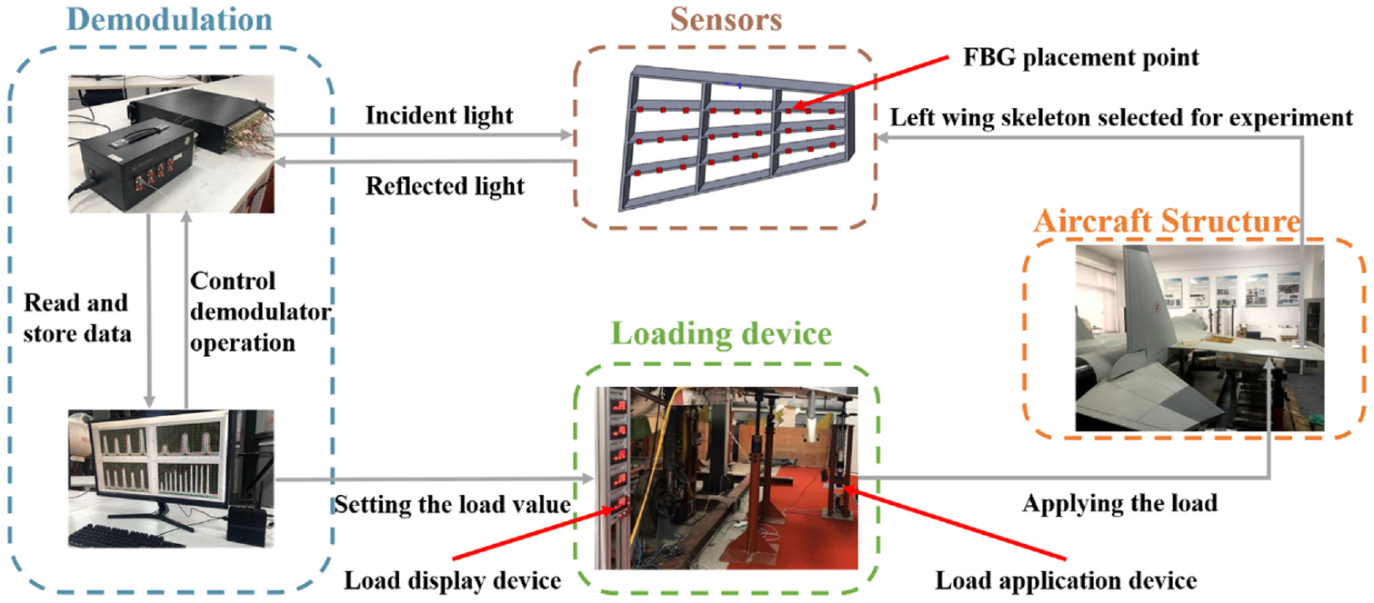
Data acquisition system.
Specifically, we selected 27 strain monitoring points combined with the layout of the aircraft wing structure. The monitoring points are all distributed in the stress concentration and damage prone areas of the aircraft wing structure, and the distribution locations are shown in Figure 2. The loading device applies a force in the vertical upward direction to a point on the aircraft wing structure. A multi-channel demodulator is used to demodulate the spectral signals of all monitoring points simultaneously. A computer connected to the demodulator is responsible for controlling the operation of the demodulator, reading and saving the experimental data. Data is transmitted between the demodulator and the computer through network cables.
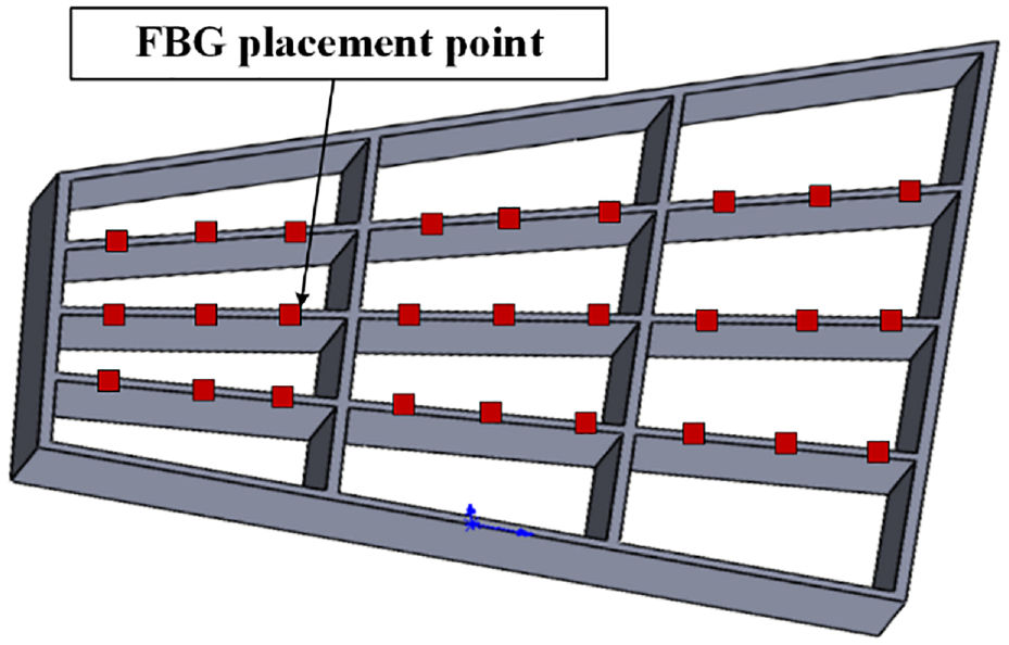
Strain sensor layout map.
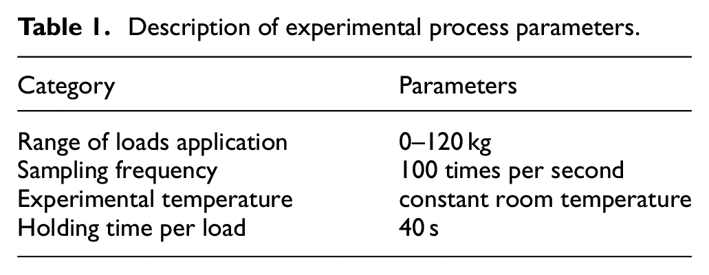
The parameters of the experimental procedure are shown in Table 1. The experiments were carried out at constant room temperature (25°C) with the aim of reducing the effect of temperature on the sensor (such as the generation of test errors). 13 To simplify the later calculations, the buckling and torsion of the aircraft wing skeleton structure are not considered in this experiment. 14 The detailed procedure of the experiment is described as follows: first, the experimental equipment is turned on under the premise of ensuring a stable environment and confirming that the loading device is in the zero-loading state; then, the loads are continuously increased, during which the deformation of the aircraft wing needs to be closely monitored to ensure that the aircraft wing is not damaged; when the loads reach the maximum value, the unloading process is carried out according to the reverse process of the loading process. Finally, the above acquisition process is repeated three times.
Description of experimental process parameters.
Data preprocessing
The data preprocessing process in this study consists of data cleaning, data conversion, data normalization and standardization. The purpose of data cleaning is to remove abnormal data as shown in Figure 3, which usually, may occur due to sensor signal fluctuations or influenced by the external environment. 15 In order to obtain more accurate measurement information and related features, the apparently abnormal data are removed by setting a threshold value, and it is necessary to note that the total amount of abnormal data removed is less than 1000th of the total experimental data in the data cleaning process.
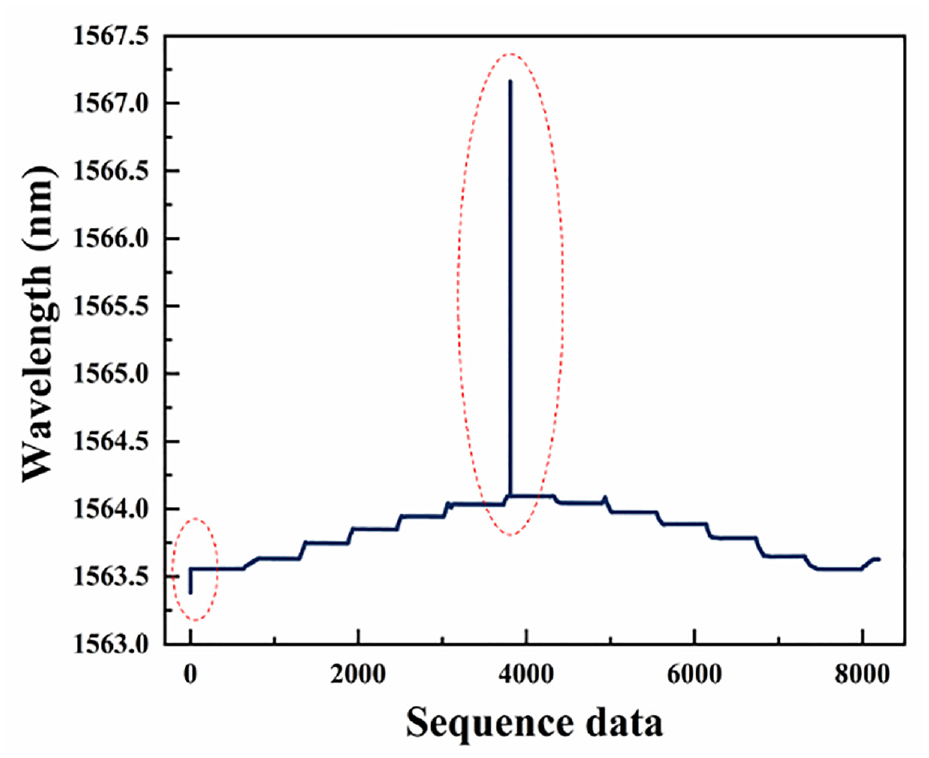
Outlier data.
Second, the data needed to be converted. The experimental data read and saved by the computer is the central wavelength of the FBG sensor, but the strain information of the aircraft wing structure is needed to calculate the loads, so the wavelength data needs to be converted to strain data. The wavelength and strain satisfy a linear relationship. 16 In this paper, the sensitivity calibration experiment yields the correspondence between wavelength data and strain as follows:

where X represents the experimentally measured wavelength data and Y represents the corresponding strain data.
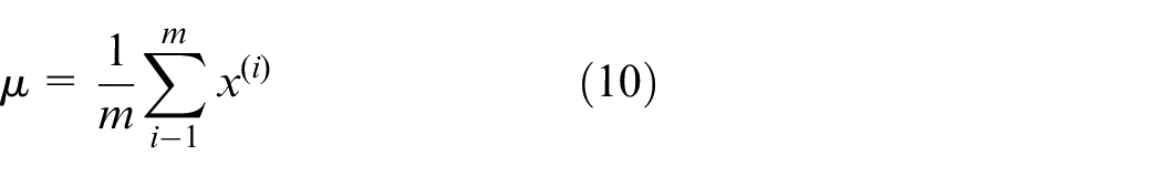
Finally, the loads and strain data are normalized and standardized respectively. The normalization of the loads data using the maximum-minimum normalization method aims to eliminate the influence of the order-of-magnitude differences in the loads data on the analysis results, and the normalization equation is:
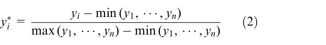
where
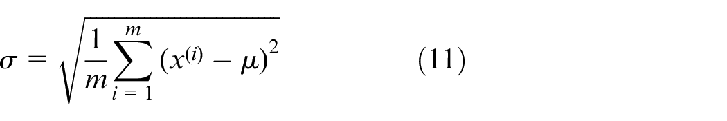
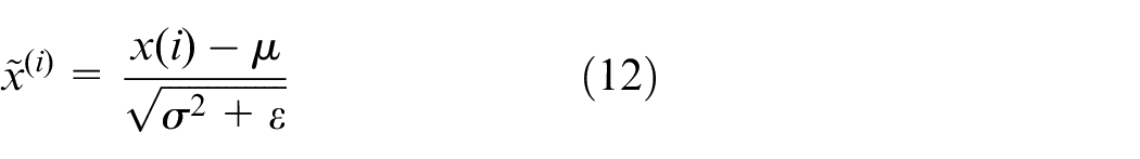
The purpose of standardization is to eliminate the influence of excessive strain differences on experimental results. The strain data are standardized using the z-Score standardization method, and the standardization equation is:
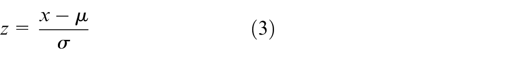
where z represents the normalized strain value, x represents the original strain value, and μ represents the mean value,
After the above data preprocessing, the total data set obtained in this study is 2706 sets of experimental data, of which 1894 sets of data are used for training the model and 812 sets of data are used as the test set to verify the model performance. The training set contains 1353 sets of data for model training and 541 sets of data as the validation set.
Method
This section first introduces the basic theoretical approach involved in the model, then gives the model proposed in this paper, and finally illustrates the training parameters of the network model.
LSTM
The load prediction can be viewed as a time-dependent problem. 17 The loads data and its corresponding strain data are long series data with time correlation, therefore, when extracting the data features, we should pay attention not only to the data spatial distribution features, but also to the data time domain features. The LSTM model is a temporal neural network model derived from recurrent neural network (RNN), on which forgetting gate, output gate and output control unit are introduced to control the iterative state. 18 It uses memory blocks to replace traditional neurons in hidden layers, which improves its ability to deal with both long-term and short-term dependency problems. 19 Therefore, the LSTM network can be considered as a network model suitable for solving load calculation problems. The general structure of the neurons of the LSTM model is shown in Figure 4. Firstly, the information to be discarded is determined by the forgetting gate, which is calculated as:

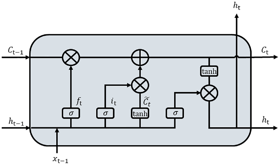
LSTM neuron structure.
where
Subsequently, the input gate as well as a tanh layer together select the new information to be stored in the cell state, which is calculated as:


where
The control of the forgetting and output gates allows the LSTM model to use the past loads information and strain information to predict the loads at the current moment. The final output of the LSTM model is the result of multiplying the output gate with the tanh layer result, which is calculated as:


where
ResNet
Theoretically, the deep neural networks should achieve better training results compared to shallow models, but in practice, this is not always the case because of the network degradation problem during deep neural network training. The network degradation problem is mainly due to the fact that deep networks contain a large number of nonlinear variations, and each nonlinear variation may cause the loss of feature information.
20
To address the problem of network degradation in deep networks, He et al.
21
proposed the residual network (ResNet) in 2015, which uses cross-layer constancy to alleviate the training difficulty of deep networks. The original intention of the residual neural network is to deepen the network so that the training result can be at least equal to that of the shallow network, which means that the constant mapping of
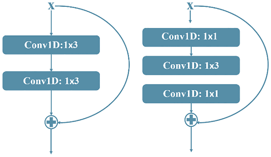
(a) Normal residual structure and (b) bottleneck residual structure.
The bottleneck residual network is an optimized version of the ordinary residual network, 22 and its core idea is to use multiple small convolutional kernels instead of one large convolutional kernel to reduce the computational effort. The structure of the bottleneck residual network is shown in Figure 5(b), which uses a convolutional layer with one convolutional kernel of 1 to dimensionally reduce the data features, so that the subsequent convolutional layer with three convolutional kernels can be more intuitive and effective for data training and feature extraction, and finally a convolutional layer with one convolutional kernel of 1 is used to reduce the dimensionality of the data features. The bottleneck residual network uses two convolutional layers with 1 convolutional kernel to reduce the dimensionality of the data features, which not only maintains the computational accuracy but also reduces the computational effort.
LSTM-ResNet
Strain data is a long series data with time dependence, and as mentioned above, LSTM has strong analysis capability for this kind of data. However, LSTM only extracts the information of temporal features of the data, while loads data and strain data contain not only temporal features but also spatial features. Convolutional neural networks can continuously extract the spatial features of strain data through nonlinear mapping. 23 Therefore, combining the above theoretical methods, this paper proposes a long short-term memory residual (LSTM-ResNet) neural network model for loads calculation, which uses the combined structure of LSTM model and ResNet model to extract features from the data. The general framework of the LSTM-ResNet model structure is shown in Figure 6, which includes a 1D-CNN layer, the LSTM network layer, the residual network layer and a fully connected layer. The input of the neural network is the applied loads and its corresponding strain value, and the output is the loads predicted by the LSTM-ResNet model.
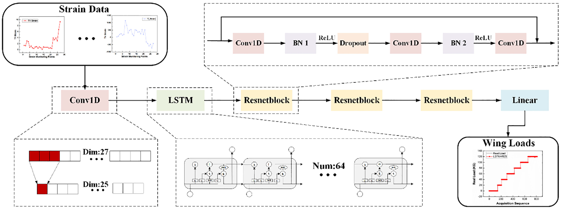
Structure of LSTM-ResNet network structure.
The main network layer parameters of the LSTM-ResNet network model are shown in Table 2. The optimal parameter combination of the combined network is determined by the ablation experiments. The input data of the network are the pre-processed strain data
where
LSTM-ResNet network structure.
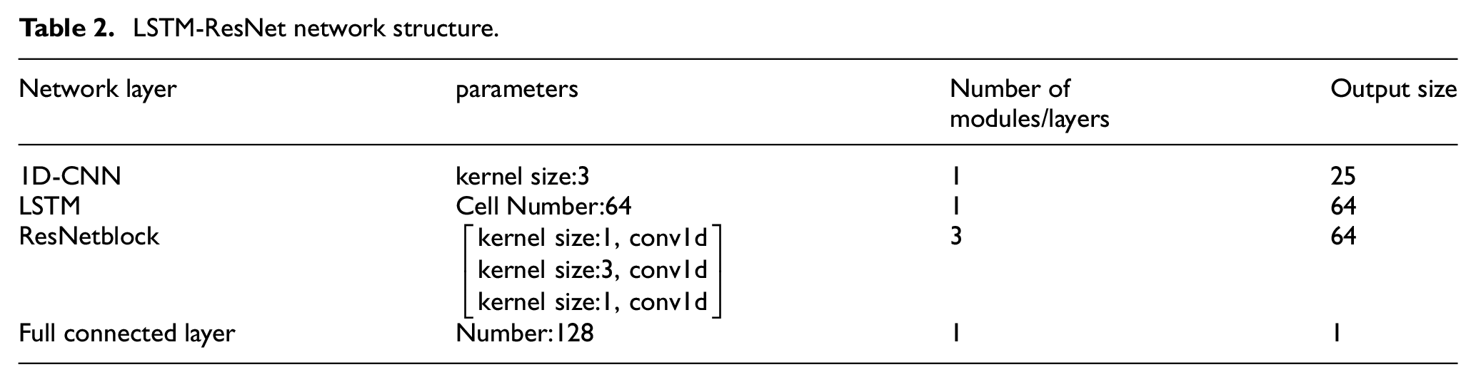
The role of dropout layer is to reduce the number of intermediate features, so as to discard some redundant information and reduce the complex co-adaptive relationship between neurons, thereby achieving the effect of avoiding the appearance of overfitting phenomenon.
25
The dropout layer in the LSTM-ResNet model has a dropout rate of 0.5. To increase the depth of the neural network and improve the neural network performance, three identical ResNetblock together form a residual network layer with an output result dimension of
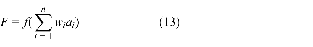
where
The activation function used in this paper is the ReLU activation function, and its expression is:

The ReLU activation function does not involve complex exponential operations and is computationally simple. In addition, the ReLU activation function causes the output of a portion of neurons to be zero, so that it causes the sparsity of the network and reduces the dependencies between parameters, and can effectively alleviate the occurrence of overfitting. 26
Neural network training
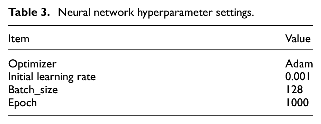
The neural network hyperparameters are shown in Table 3. Neural network superparameters include learning rate, batch size, optimization method and iteration times. In this paper, grid search method is used to determine the learning rate, batch size and other parameters. The optimizer used in the model training is the Adam optimizer, which is a first-order gradient optimization algorithm. The Adam optimizer is computationally efficient and has a low memory requirement and is suitable for problems with non-smooth objectives and with noise. 27
Neural network hyperparameter settings.
The loss function used in the training process is the mean square error (MSE) loss function, which is defined as:
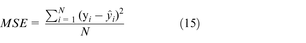
where
The MSE is a commonly used loss function, and the function curve of the MSE is smooth and continuous and derivable everywhere, and as the error decreases, the gradient also decreases, which is conducive to fast convergence. 28 Figure 7 shows the loss function curves of the training process and the validation process. It can be seen from Figure 7 that both curves converge and have little difference, which proves that there is no overfitting or underfitting in the model.
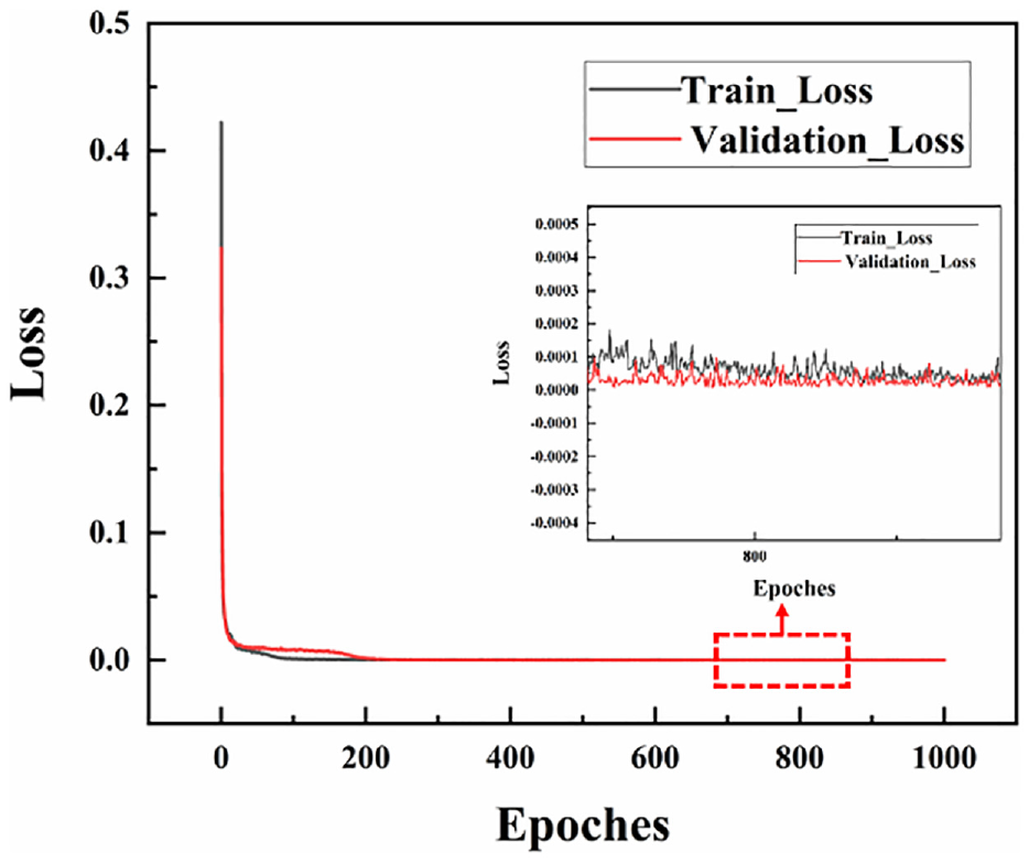
LSTM-ResNet network model loss function.
Results
To validate the performance of the LSTM-ResNet model, firstly, the evaluation metrics used for model evaluation are presented. Secondly, the performance of the model on the test set is described. Finally, the results of the model and other methods on the test set are compared and analyzed.
Evaluation methodology
In this paper, relative error and variance are used to assess the degree of model deviation and dispersion, and to measure the accuracy of the model by both types of metrics. The relative error can show the degree of deviation of the data from the true value and thus visually compare the accuracy of different models for the loads calculation problem. 29 The relative error is calculated as:
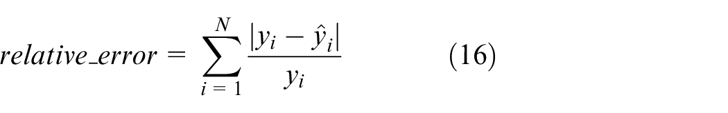
where
On the basis of relative error, the performance of all models is compared using the average relative error as an evaluation criterion. The average relative error can better judge the overall effect of the model compared to the relative error. The average relative error formula is:
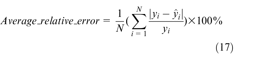
where
Variance is an evaluation criterion to measure the degree of dispersion of the data; the larger the variance, the greater the dispersion. 30 For the model, a smaller variance means that the model is more stable and the prediction results are more reliable. The variance formula is:
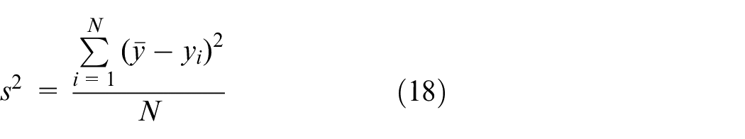
where
Experimental results
The comparison results between the real loads and the predicted values of the LSTM-ResNet model are shown in Figure 8. The data volume in the figure is large, thus only part of the data is expanded in detail to show. From the experimental results in Figure 8, we can see that all the prediction results of the LSTM-ResNet network model are close to the real loads, and the error of the loads prediction results is kept within 0.2 kg, and the average relative error of the model prediction results is only 0.08% through calculation. The experimental results show that the LSTM-ResNet model has not only the extraction capability of LSTM network for time-domain features, but also the extraction capability of residual network for spatial features, so the LSTM-ResNet network has a high accuracy. However, we can see from Figure 8 that the model has significant deviation in the prediction results for two groups of edge loads, 0 and 120 kg. Among them, the prediction results of the model for the loads of 0 kg as a whole are obviously higher than the real value, while there are some deviations in the prediction results for the loads of 120 kg.
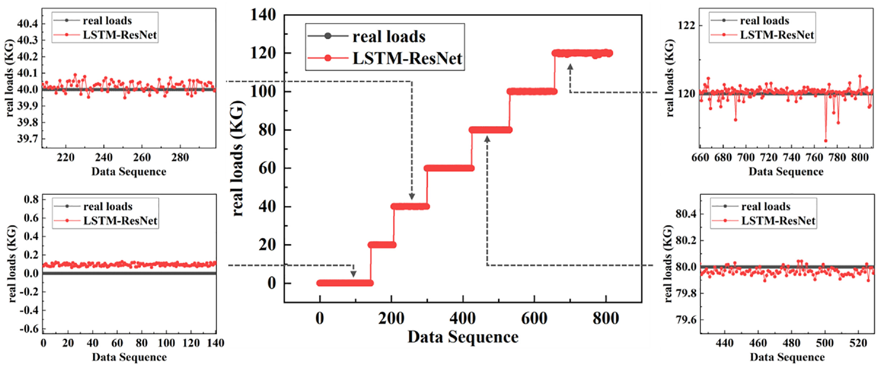
Prediction results of LSTM-ResNet model compared with the real loads.
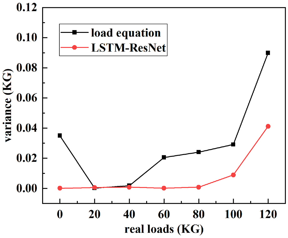
To explore the reasons leading to this result, we further compared the variance of the predicted results for each group of loads. The variance comparison results are shown in Figure 9, from which it can be seen that the variance of the model’s prediction results at 0 kg is not significantly higher. Therefore, we infer that the error in the prediction results at 0 kg is due to the fact that although no loads are applied to the aircraft wing structure at 0 kg, a weak background noise is generated due to the environment and the aircraft wing structure itself, and thus its prediction results have an overall deviation compared to the real loads. However, when the loads start to be applied, this part of the background noise is small for the applied loads. Therefore, the background noise does not have a significant effect on the prediction of other loads. There are some significant deviations in the predictions of the model for the 120 kg loads, and the variance of 120 kg is significantly higher as can be seen in Figure 9. We randomly selected a strain monitoring point and performed variance calculation on its strain data to judge the stability of the experimentally collected data. The results of the strain data variance calculation are shown in Figure 10, and the strain data under 120 kg loads also showed a large degree of dispersion. As a result, we inferred that the strain data under 120 kg were more discrete due to the experimental structure itself, which led to a larger error in the prediction results.
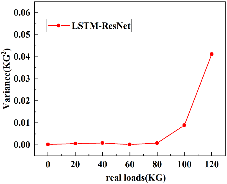
LSTM-ResNet variance results.
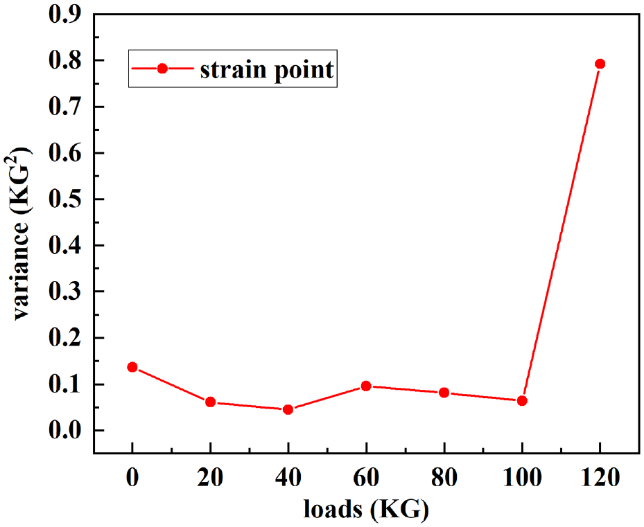
Strain value variance at any point on the aircraft wing skeleton.
Comparison results with the load equation
The traditional method for the aircraft loads calculation is the load equation, 31 which uses known strain data and corresponding loads to determine the equation coefficients, and subsequently uses the strain data to bring into the equation to derive the unknown loads. The load equation is given as:

where A is the measured strain matrix,
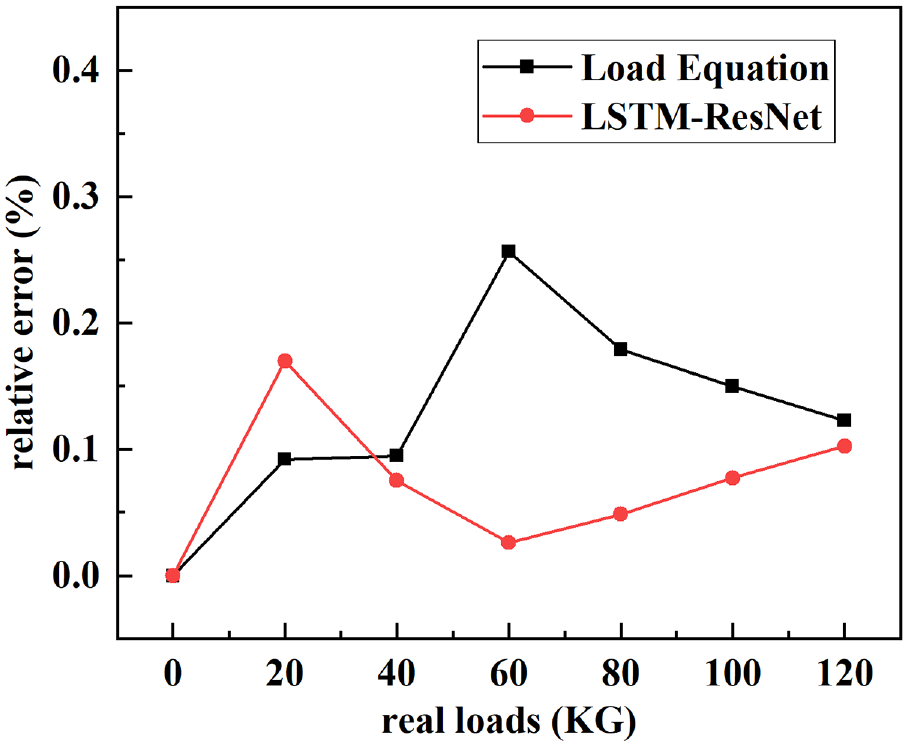
To verify the performance of the LSTM-ResNet algorithm, the predictions were performed on the same data set using the load equation and the LSTM-ResNet model, respectively. From the average relative error comparison results in Figure 11, we can see that the LSTM-ResNet model has a higher prediction accuracy, and the average relative error of its prediction results is only 0.08%. As shown in Figure 12, the relative error results of the prediction of the LSTM-ResNet model for loads above 40 kg are smaller than those of the load equation. Although the average relative error of the loads prediction results is smaller for the load equation below 40 kg, its overall prediction results are less stable. From the variance comparison results shown in Figure 13, it can be seen that the stability of the LSTM-ResNet model is significantly higher than that of the load equation. Combining the above comparison results, we can infer that although both the load equation and LSTM-ResNet model can be used to solve the load calculation problem, the LSTM-ResNet model is more suitable for solving the load calculation problem of nonlinear systems in practical environments, and its overall error is smaller and the stability of prediction results is higher. The activation function in the LSTM-ResNet model enables a nonlinear transformation, which improves the model’s ability to recognize loads.
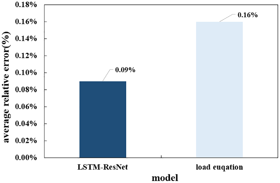
Comparison results of relative error between LSTM-ResNet model and load equation.
Comparison results of relative error between LSTM-ResNet model and load equation.
Comparison results of variance of LSTM-ResNet model and load equation.
Comparison with other neural networks
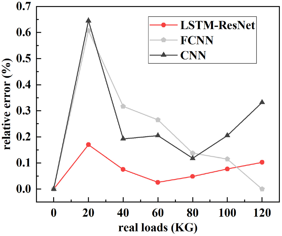
In order to verify the performance of the LSTM-ResNet model, it was compared with other deep learning models for training under the same data set. The average relative error shown in Figure 14 and the comparison results of the relative error shown in Figure 15 show that LSTM-ResNet model has a significantly better accuracy than other deep learning models. The variance comparison results shown in Figure 16 also show that the stability of LSTM-ResNet model is also better than other deep learning models. It can be inferred that, although all neural network models can carry out load calculation, other neural network models only pay attention to spatial or temporal dimension features, while LSTM-ResNet model pays attention to both temporal and spatial feature information, so its predicted value is closer to the real load value. In addition, as the LSTM-ResNet model is a deep neural network model, compared with the traditional neural network model, its generalization ability is improved with the deepening of the network.
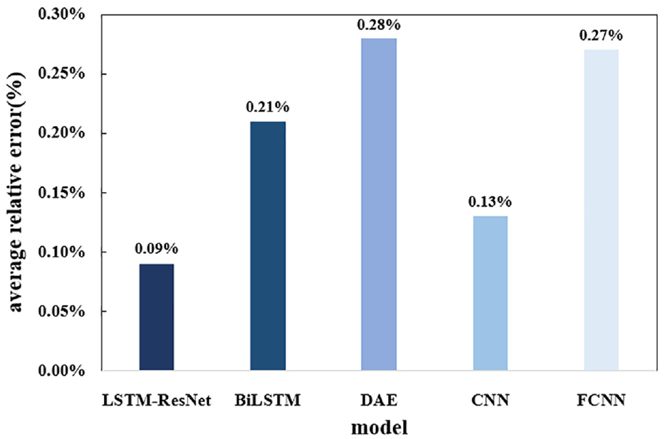
Comparison results between LSTM-ResNet model and other deep learning models.
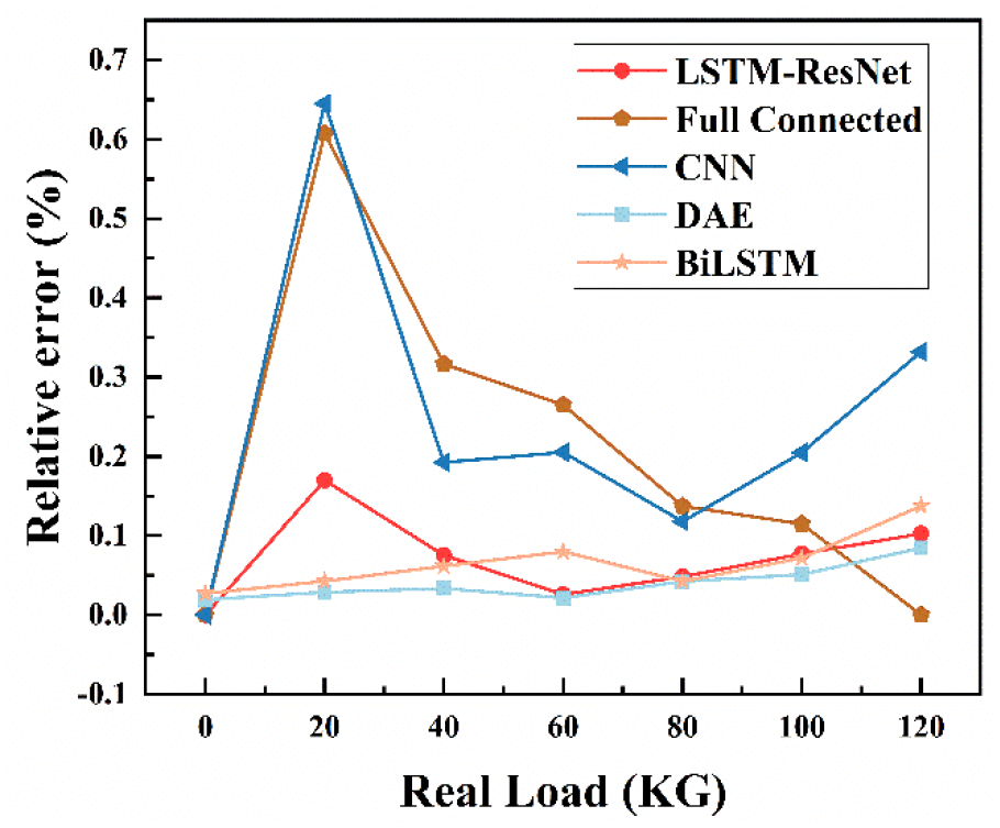
Results of the relative error of LSTM-ResNet model compared with other deep learning models.
Comparison results of LSTM-ResNet model with other deep learning models variance.
Comparison with ResNet and LSTM
To verify that the LSTM-ResNet model has higher accuracy of loads computation compared with the original network, we train and validate the traditional bottleneck residual network, LSTM network, and LSTM-ResNet model on the same dataset using the same parameters, respectively. Then, the evaluation results of the LSTM-ResNet model are compared with those of the traditional bottleneck residual network and the LSTM model. The relative error comparison results shown in Figure 18 show that the other two models have significant advantages over the ResNet model using only the traditional bottleneck structure. Figure 19 also proves that the loads prediction results of the ResNet model using only the traditional bottleneck structure are less stable. From the above comparison results, we can conclude that deep neural networks are more suitable for solving complex nonlinear loads problems like aircraft wing loads calculation. In addition, the average relative error comparison results shown in Figure 17 show that the LSTM-ResNet model has a higher accuracy of loads calculation, from which we can infer that although all three models are used to deal with nonlinear regression problems, compared with the LSTM-ResNet model, the LSTM model focuses only on the information of data temporal features and the ResNet network focuses only on the information of data spatial features. The LSTM-ResNet model can take into account both temporal and spatial features, so the accuracy of loads calculation is higher.
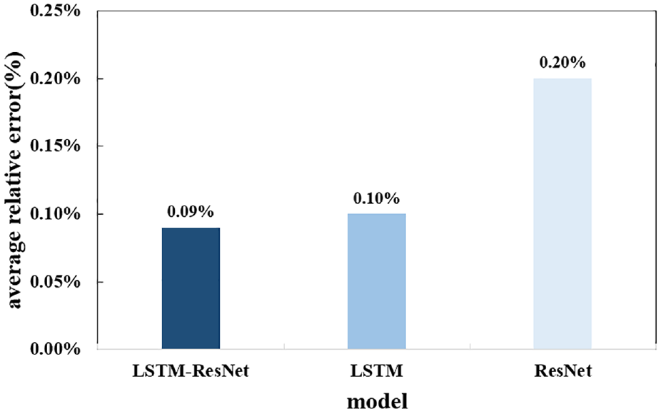
Results of LSTM-ResNet model compared with the average relative error of ResNet and LSTM.
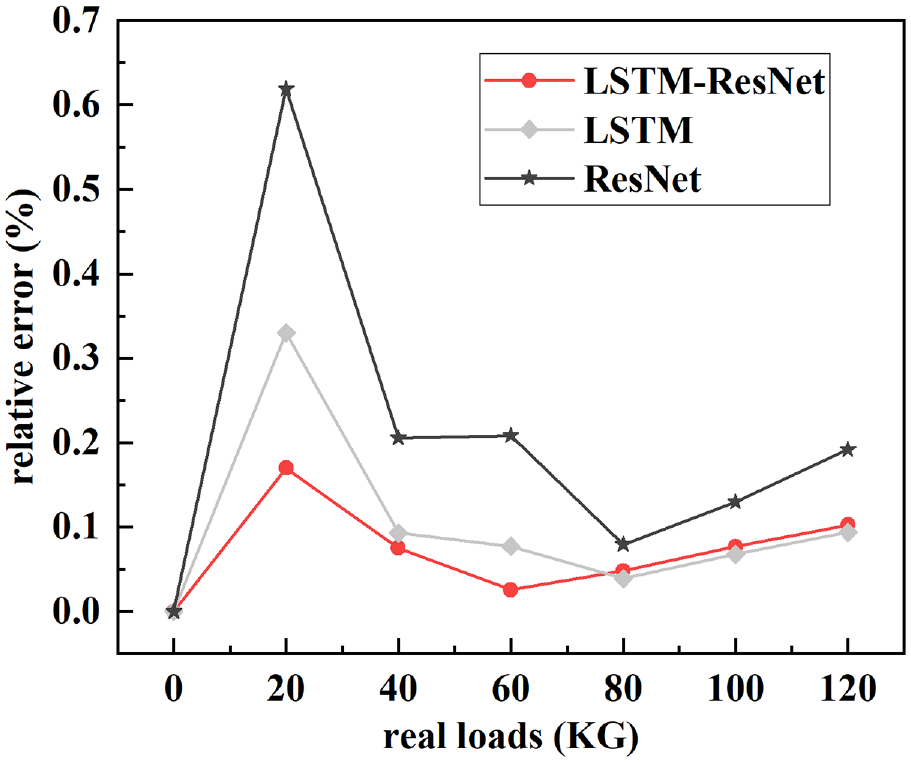
Results of the relative error of LSTM-ResNet model compared with ResNet and LSTM.
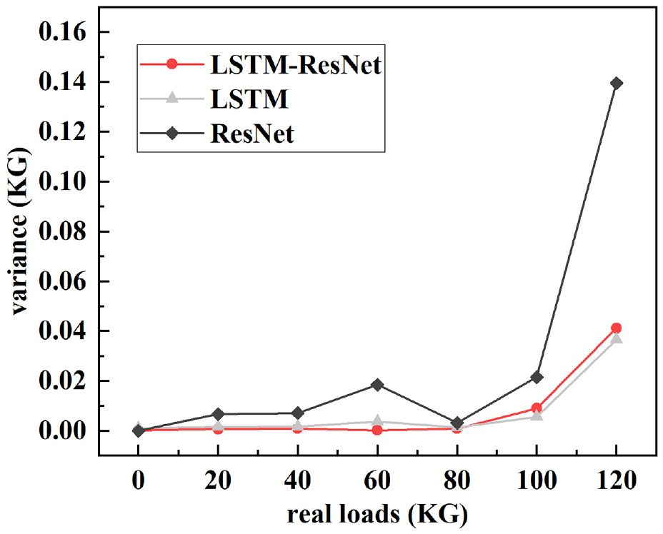
Comparison results of LSTM-ResNet model with ResNet and LSTM variance.
Comparison with machine learning methods
At present, there are also researchers using machine learning methods (such as SVM) for load calculation. 32 In order to verify that the LSTM-ResNet model has a higher load calculation accuracy than the machine learning method, we conducted training and verification on the SVM model and the LSTM-ResNet model respectively on the same data set. Then, the evaluation results of the LSTM-ResNet model were compared with those of the SVM model. The comparison results of average relative errors shown in Figure 20 show that the LSTM-ResNet model has a higher load calculation accuracy. As can be seen from the comparative results of relative errors shown in Figure 21, the SVM model has a large prediction error on the edge load. It also can be seen from the variance comparison results shown in Figure 22 that the LSTM-ResNet model has smaller variance, which means that the prediction results of the LSTM-ResNet model are more stable. It can be inferred that deep learning methods have better generalization ability compared to machine learning methods, and deep learning methods can learn the features of the data better. Therefore, compared to machine learning methods, deep learning methods have higher accuracy in load calculation problems.
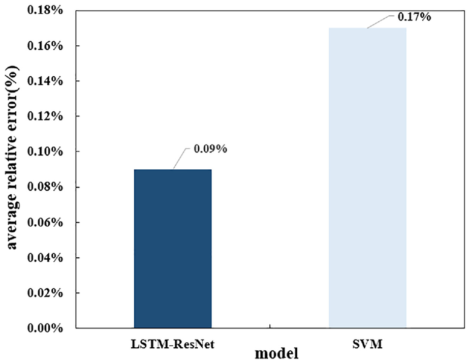
Results of LSTM-ResNet model compared with the average relative error of SVM.
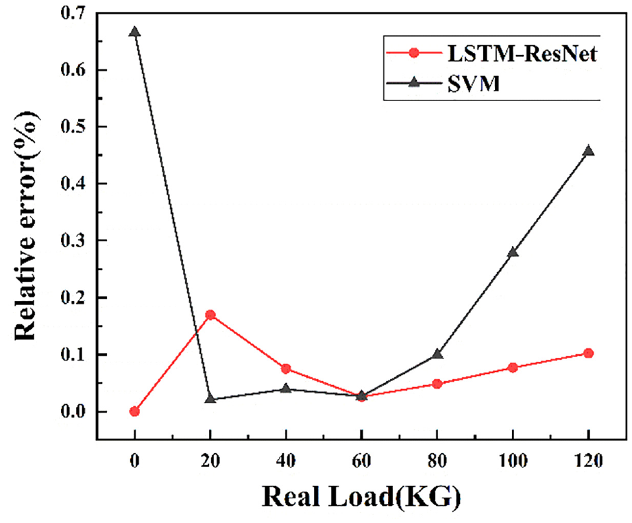
Results of the relative error of LSTM-ResNet model compared with SVM.
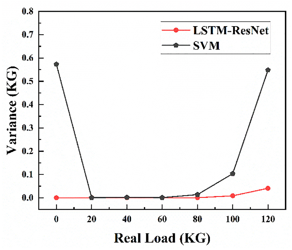
Comparison results of LSTM-ResNet model with SVM variance.
Discussions and conclusion
Currently, the more commonly used method in the engineering practice of loads calculation is the load equation. However, because the load equation is a multiple linear regression method, it is mostly calculated by simplifying the aircraft structure as an ideal elastic system, which is not enough for the nonlinear representation of the data. And although the deep learning algorithm can compensate for the lack of nonlinear fitting ability of the load equation, the existing deep learning algorithms mostly use a single structured neural network for loads calculation, and in this case, the time domain features of strain data and loads data are often neglected. For overcoming the above limitations, this paper proposes a long and short-term memory residual network (LSTM-ResNet) loads calculation model for predicting aircraft wing loads. In order to verify the model performance more accurately, this study uses an aircraft wing skeleton as the test structure, and designs an experimental scheme for aircraft wing strain data and loads data acquisition, combining FBG sensing technology to collect the data. Subsequently, the collected data are preprocessed and fed into the LSTM model and the ResNet model to extract the spatio-temporal characteristics of the data and predict the loads. In this paper, we compare the LSTM-ResNet model with other existing loads calculation methods under the same data set, and the experimental results show that the average relative error of the LSTM-ResNet model is only 0.08%. Compared with other existing loads calculation models, the proposed model in this paper can predict the loads value corresponding to the strain more accurately, and thus the proposed method in this paper can provide a new technical potential for future loads calculation engineering.
Although LSTM-ResNet model proposed in this paper can be effective in the calculation of aircraft wing loads and demonstrates a competitive accuracy compared to existing methods. However, the experiments and data mentioned in this paper are subject to certain limitations: (1) The research covered in this paper has insufficient amount of data that can be collected due to the problem of experimental constraints, with data available for only 27 strain monitoring points. (2) The prediction results of the neural network model designed in this paper are more discrete and less stable at 120 kg. (3) In order to obtain better training results before model training, we need to manually preprocess the collected data.
In the subsequent research, first of all, we need to collect more data in the early data acquisition experiment to verify the model more completely. Secondly, we can investigate the use of data augmentation to compensate for the insufficient amount of data due to the limitation of the wing structure and the limitation of the experimental environment. Finally, we need to optimize the model to improve the stability of the model under the edge load value and make the model more reliable.
Footnotes
Declaration of conflicting interests
The author(s) declared no potential conflicts of interest with respect to the research, authorship, and/or publication of this article.
Funding
The author(s) disclosed receipt of the following financial support for the research, authorship, and/or publication of this article: This work was supported by R&D Program of Beijing Municipal Education Commission [grant number: KM202011232007], Program of Promoting of Beijing Information Science and Technology—Diligence Talents [grant number: 5112111145], Foundation of Beijing Laboratory of Biomedical Detection Technology and Instrument [grant number: 9142123202]. We thank all the participants who have participated in this work.