Fault diagnosis of PLC-based discrete event systems using Petri nets

Abstract

This paper addresses the fault diagnosis problem of PLC-based systems that can be modeled as Petri nets under a certain level of abstraction. The existing Petri-net-based fault diagnosis approaches often associate transitions and/or places with sensors and require that any change in sensor readings needs to be treated by a PLC, leading to a situation that the PLC would be too busy processing the changes in sensor readings to perform other tasks. This paper assumes that a PLC does not monitor the changes of readings of sensors all the time, but periodically reads the values of sensors when needed. The system output is defined as a marking sequence interleaved with possible observed transitions. A fault diagnosis algorithm is developed by defining and solving integer linear programing (ILP) problems whose size is regardless of the length of the system output. The proposed approach enjoys high computational efficiency compared with other ILP-based approaches and is more suitable for fault diagnosis of PLC-based systems with low computing power.

Introduction

Position of this paper

The rapid development of electronic technology has made the computer-integrated systems, which can be abstracted as discrete event systems (DESs), ¹ more and more complex, structurally and functionally. Fault diagnosis aims to ensure the safe and stable operation of these systems by detecting and isolating faults as soon as possible (In this paper, “failure” and “fault” have the same meaning and we use them interchangeably. However, they may have slightly different meanings in some publications). More specifically, fault diagnosis requires to complete three tasks: fault detection, fault isolation, and fault identification, corresponding to determining if a system is running normally, revealing the locations and numbers of faults, and identifying the specific nature of faults, respectively.^2–5

In real industrial systems, the control of a system can often be implemented by a programmable logic controller (PLC). In general, a PLC consists of a central processing unit, a storage unit, and an input-output unit, and can receive, send and process various electronic signals. A PLC is connected to the sensors distributed on the components of a system such that it can collect the control parameters of the system by reading these sensors. Many existing fault diagnosis approaches in the literature can be implemented with PLCs.

In the domain of DESs, many existing fault diagnosis approaches have two main disadvantages: (i) a number of approaches^6–9 have exponential computational complexity in the worst case and their computational cost may be prohibitive for large systems and (ii) some approaches^10–12 require that any change in sensor readings needs to be treated by a PLC such that the PLC would be too busy processing the changes in sensor readings to perform other tasks.

To overcome these disadvantages, we propose a fault diagnosis approach which equips a system with more sensors and reads sensors at a fixed time interval. The proposed approach has higher computational efficiency and is more appropriate for use in real-world systems with low computing power. On the other hand, the main drawback of the proposed approach is the higher cost of purchasing sensors and the higher difficulty of deploying them.

Differently from the Petri-net-based approach proposed in this paper, some other approaches based on structural analysis^13,14 or fault trees^15,16 are also exposed. In contrast to actively detect and isolate faults in this paper, the stability property of a system is explored in Foroozanfar et al. ¹⁷ and Lutz-Ley and Lopez-Mellado. ¹⁸ A stable system can automatically return to a normal state from a fault state in finite number of steps. Before presenting the details of the proposed approach, we review some typical publications on fault diagnosis of DES.

Some original theoretical results for fault diagnosis are exposed based on automata. In Sampath et al., ⁶ a plant is modeled as an automaton in which faults are represented by unobservable events and each observable event is associated with a sensor. A diagnoser for fault diagnosis is constructed offline by an algorithm with exponential complexity. When an event is observed, by inspecting the diagnoser, the fault state of the plant may be one of three cases: faults do not occur, faults may have occurred, and faults must have occurred. This fault diagnosis approach is applied to a realistic HVAC system in Sampath et al. ¹⁹

In contrast to automaton models, Petri nets, as a typical mathematical model of DESs, have been widely used in supervisory control,^20–23 performance optimization,^24–26 and model identification^10,11,27,28 because of their intrinsic distributed features and efficiency in handling large systems. Simultaneously, in recent decades, many fault diagnosis approaches based on Petri nets have also been reported, which can be generally categorized into two classes.

In the first class, the sensors are equipped with observable transitions and the output of a system is defined as a sequence of observable transitions. Integer linear programing (ILP) problems often need to be built and solved for performing fault diagnosis. In Dotoli et al., ⁷ an online fault diagnosis approach is reported that builds an ILP problem based on the observed transition sequence. By assigning two different objective functions to the ILP problem and solving it, whether a fault has occurred can be determined. This approach is extended to the case of labeled Petri net in Fanti et al. ⁸ and Zhu et al. ²⁹

Basile et al. ³⁰ deal with the fault diagnosis problem by means of the notion of generalized markings, that is, markings in which the number of tokens can be a negative integer. By solving an ILP problem built according to the negative elements of a generalized marking, the occurrence of a fault can be deduced. Wang et al. ³¹ employ generalized markings to backward conflict-free Petri nets and propose a more efficient fault diagnosis approach by constructing an ILP problem with smaller size.

In Giua and Seatzu, ³² the notion of basis markings is first defined and a fault diagnosis approach based on basis markings is proposed. Given an observed transition sequence, the corresponding basis markings are computed by an algorithm using only algebraic manipulations. The diagnosis result of a fault is obtained by checking the basis markings and, if necessary, solving some ILP problems. The notion of basis markings is further extended to basis reachability graphs in Cabasino et al.^9,33 where a basis reachability graph is first constructed offline and then an online diagnosis algorithm is developed by inspecting the basis reachability graph at each step.

In the second class, the sensors are equipped with observable transitions as well as certain places of a Petri net. The system dynamic is represented as an observable transition sequence or a transition-marking sequence. In Zhu et al.,^10,11 faults are described by unobservable transitions not contained in the initial net model of a plant and the output of a system is defined as an observed evolution, that is, a transition-marking sequence. By solving an ILP problem constructed based on the observed evolution, the unobservable transitions are identified that characterize the number and locations of faults.

Ru and Hadjicostis ¹² model systems as partially observed Petri nets (i.e. nets equipped with transition and place sensors) and define the system output as an ordered sequence of three tuples $(M,t,M\prime )$ ’s, where $M$ and $M\prime$ are two markings and $t$ is a transition. After transforming the partially observed Petri net into a labeled net, they propose an online fault diagnosis algorithm based on reachability graph analysis of the unobservable subnet of the labeled net. The study in Lefebvre ³⁴ also utilizes partially observed Petri nets and provides an efficient fault diagnosis algorithm by solving a number of linear matrix inequalities. The number of times of solving inequalities is linear in the length of an observed sequence.

In Ramirez-Trevino et al., ³⁵ a bottom-up modeling methodology is explored to build an interpreted Petri net (IPN) model of a system. By dividing the set of places into a subset of places modeling fault states and a subset of places modeling normal states, the diagnosability of the built IPN is formally defined and a scheme for detecting and locating fault states is developed. By assuming that all places are observable, Genc and Lafortune ³⁶ extend the diagnoser approach based on automata in Sampath et al. ⁶ to the context of Petri nets. A Petri net diagnoser is constructed to perform online diagnosis. This approach is of high computational complexity since the marking enumeration upon observing an transition at each step is needed.

The study in Pencole and Subias ³⁷ explores the diagnosability of safe labeled time Petri nets based on the notion of event patterns. An efficient approach of determining diagnosability of a safe Petri net is reported by means of model-checking techniques. Al-Ajeli and Parker  propose a fault diagnosis approach for labeled Petri nets based on Fourier-Motzkin elimination. A diagnoser in the form of sets of inequalities is first constructed offline and then online fault diagnosis is performed by checking the constructed diagnoser when observing an event. This approach provides a better trade-off between the size of the diagnoser and diagnosis time. In recent years, some extended versions of fault diagnosis are studied, such as robust diagnosis, ³⁸ diagnosability enforcement, ³⁹ and synchronous diagnosis.^40,41 Two comprehensive surveys on fault diagnosis can be found in Al-Ajeli and Parker ⁴² and Lafortune et al. ⁴³

Contributions

As already mentioned above, the first class of fault diagnosis approaches often needs to solve ILP problems whose size is linear or polynomial with respect to the length of the observed sequence. When the observed sequence is very long, these approaches become computationally prohibitive. On the other hand, the second class of approaches generally assumes that all or part of places are observable, that is, these places are equipped with sensors. Moreover, the approaches in the second class usually require that any change in the readings of place sensors needs to be treated by a PLC. A Petri net model of a real-world system may include a large number of places and there are a deluge of changes of sensor readings during the operation of the system. The PLC would be too busy processing the changes in sensor readings to perform other tasks. Consequently, in some cases, the existing fault diagnosis approaches are not applicable to real-world systems.

In this paper, we assume that part of transitions and all places are equipped with sensors. In addition, due to the limited processing power of a PLC, we assume that it does not monitor the changes of readings of place sensors all the time, but periodically reads the values of the sensors when needed. The system output is defined as a marking sequence interleaved with possible observed transitions.

Based on the observed system output, a fault diagnosis algorithm is developed by defining and solving ILP problems whose size is regardless of the length of the system output. Thus, the computational cost of the algorithm will not increase with the increase of the length of the system output. Namely, the algorithm enjoys a high computational efficiency for those systems that satisfy the assumptions made in this paper. On the other hand, since the PLC only requires to read place sensors once in a time period and does not monitor the changes of sensor-readings all the time, the proposed algorithm is more suitable for fault diagnosis of some PLC-based systems.

This paper is organized as follows. In Section 2, some basic definitions on Petri net are provided. In Section 3, the problem to be addressed is formally defined and a solution to the problem is reported in Section 4. In Section 5, we extend the fault diagnosis algorithm for Petri nets to the case of labeled Petri nets. To show the effectiveness of the proposed approach, in Section 6, we apply the approach to a case study example. Finally, a conclusion is drawn in Section 7.

Basic definitions

In this section, we introduce the definitions and notations used throughout the paper. For the complete details of Petri nets, the reader is referred to Giua and Silva ⁴⁴  and Murata. ⁴⁵

A Petri net is a bipartite graph represented as a four-tuple $N=(P,T,\mathrm{Pre},\mathrm{Post})$ , where $P$ is a set of $m$ places, $T$ is a set of $n$ transitions with $P\cup T\ne \varnothing$ and $P\cap T=\varnothing$ , $\mathrm{Pre}:P\times T\to \mathbb{N}$ ( $\mathbb{N}$ is the set of non-negative integers) and $\mathrm{Post}:P\times T\to \mathbb{N}$ are two functions represented as two matrices, which specify the arcs of the graph. We denote by $C=\mathrm{Post}-\mathrm{Pre}$ the incidence matrix of net $N$ . The sets of input places and of output places of a transition $t$ are denoted by ${}^{•}t=\{p\in P|\mathrm{Pre}(p,t)>0\}$ and $t^{•}=\{p\in P|\mathrm{Post}(p,t)>0\}$ , respectively. Similarly, for a place $p\in P$ , we define ${}^{•}p=\{t\in T|\mathrm{Post}(p,t)>0\}$ and $p^{•}=\{t\in T|\mathrm{Pre}(p,t)>0\}$ .

A marking of a Petri net is a mapping $M:P\to \mathbb{N}$ . The number of tokens in a place $p\in P$ at a marking $M$ is represented by $M(p)$ . A marking $M=[x_1,\dots ,x_m{]}^T$ is written as $M=x_1{p}_1+\cdots +x_m{p}_m$ (the items whose coefficients are zero are omitted) for simplicity. By associating a Petri net $N$ with an initial marking $M_0$ , a Petri net system $〈N,M_0〉$ is defined.

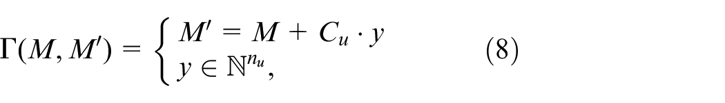
A transition $t\in T$ is said to be enabled at marking $M,$ denoted by $M[t〉,$ if the number of tokens in each input place of $t$ is greater or equal to the weight of the corresponding arc, that is, $M(p)\ge \mathrm{Pre}(p,t)$ for all $p{\in }^{•}t.$ With a slight abuse of notation, we use $M[\sigma 〉$ to denote that a transition sequence $\sigma \in T^{*}$ is enabled at marking $M.$ A marking $M_{\alpha }$ is reachable from $M$ after firing $\sigma$ , denoted by $M[\sigma 〉M_{\alpha }$ . In addition, $M_{\alpha }$ is computed by the state equation of a net

$$M_{\alpha }=M+C·\mathrm{\pi }(\sigma ),$$

(1)

where $\mathrm{\pi }$ is a function, defined by $\mathrm{\pi }:T^{*}\to {\mathbb{N}}^n$ , which computes the Parikh vector of a transition sequence $\sigma$ . If a transition $t$ is in $\sigma$ , we write $t\in \sigma$ for simplicity.

The set of transition sequences that are enabled at the initial marking $M_0$ is defined as

$$\mathcal{L}(N,M_0)=\{\sigma \in T^{*}|M_0[\sigma 〉\}.$$

(2)

The reachability set, represented as $R(N,M_0)$ , of a net system contains all markings that are reachable from $M_0$ by firing a transition sequences $\sigma \in \mathcal{L}(N,M_0),$ that is, $R(N,M_0)=\{M\in {\mathbb{N}}^m|(\exists \sigma \in T^{*})M_0[\sigma 〉M\}.$

A transition is said to be observable if it is equipped with a sensor that monitors its firing; otherwise, it is called unobservable. We denote by $T_o$ and $T_u$ the set of observable transitions and the set of unobservable transitions, respectively. In addition, the cardinalities of $T_o$ and $T_u$ are represented as $n_o$ and $n_u$ , respectively. Thus, the set $T$ of transitions is partitioned into two disjoint subsets $T_o$ and $T_u$ with $T=T_o\cup T_u$ . A place of a Petri net is said to be measurable if the number of tokens residing into it can be detected by a sensor. In this paper, we assume that all places of a Petri net are measurable. A Petri net is said to be acyclic if it does not contain any directed cycle.

• Theorem 1. ⁴⁵ A marking $M\in {\mathbb{N}}^m$ is reachable from $M_0$ in an acyclic Petri net system $〈N,M_0〉$ if and only if there exists a column vector $x\in {\mathbb{N}}^n$ such that $M=M_0+C·x$ , where $m$ and $n$ are the numbers of places and transitions, respectively.

• Definition 1. Given a Petri net $N=(P,T,\mathrm{Pre},\mathrm{Post})$ and a transition subset $\hat{T}\subseteq T$ , the $\hat{T}$ -induced subnet of $N$ is defined as $N_{\hat{T}}=(P,\hat{T},\mathrm{Pr}{e}_{\hat{T}},\mathrm{Pos}{t}_{\hat{T}})$ , where $\mathrm{Pr}{e}_{\hat{T}}$ and $\mathrm{Pos}{t}_{\hat{T}}$ are the restrictions of $\mathrm{Pre}$ and $\mathrm{Post}$ on $P\times \hat{T},$ respectively.

According to Def. 1, it is straightforward to obtain the $T_u$ -induced subnet of $N=(P,T,\mathrm{Pre},\mathrm{Post})$ , denoted by $N_u=(P,T_u,\mathrm{Pr}{e}_u,\mathrm{Pos}{t}_u)$ . We also call the $T_u$ -induced subnet the unobservable subnet of $N$ . The incidence matrix of $N_u$ is represented by $C_u=\mathrm{Pos}{t}_u-\mathrm{Pr}{e}_u$ . Unless otherwise stated, the unobservable subnet of the considered Petri nets in this paper is assumed to be acyclic.

To characterize failures in a real-world system, the unobservable transitions in $T_u$ are further divided into regular unobservable transitions, denoted by $T_{\mathrm{reg}}$ , and fault transitions, denoted by $T_f$ , that is, $T_u=T_{\mathrm{reg}}\cup T_f$ and $T_{\mathrm{reg}}\cap T_f=\varnothing$ . The fault transition set $T_f$ is partitioned into $r$ fault classes, that is, $T_f=T_f^1\cup T_f^2\cup \dots \cup T_f^r$ , and the partition is represented as ${\Pi }_f=\{T_f^1,\dots ,T_f^r\}$ . For simplicity, we say that $T_f^i$ occurs if a fault $f\in T_f^i$ takes place in a system. Given a sequence $\sigma \in T^{*}$ , we use $t\in \sigma$ to denote that $t$ is contained in $\sigma$ and $T_f^i\in \sigma$ to denote that there exists at least a transition $f\in T_f^i$ such that $f\in \sigma$ .

A Petri net system with a labeling function $\lambda :T\cup \{\epsilon \}\to E\cup \{\epsilon \}$ is called a labeled Petri net (LPN) system, denoted by $〈N,M_0,E,\lambda 〉$ , where $E$ is an alphabet and $\epsilon$ represents the empty string. The label of the empty string $\epsilon$ is itself, that is, $\lambda (\epsilon )=\epsilon$ . The set of transitions that have the same label $e$ is denoted by $T_e=\{t\in T|\lambda (t)=e\}$ . The labeling function $\lambda$ is extended to a transition sequence $\sigma =t_1{t}_2\dots t_h\in T^{*}$ with $h$ being its length by defining $\lambda (\sigma )=\lambda (t_1)\lambda (t_2)\dots \lambda (t_h)$ . We obtain the underlying Petri net of an LPN by removing all labels of transitions of the LPN.

Problem definition

In general, faults in a system can be divided into three types: incipient, intermittent, and permanent. The approach proposed in this paper is based on Petri nets (a typical discrete event model) and are appropriate for faults that cause a distinct change in the state of system components but do not necessarily bring the system to a halt. Thus, the proposed approach can be used to detect intermittent or permanent faults. These faults may originate from different system components, such as sensors, actuators, or controllers.

The problem of fault diagnosis consists in determining whether faults have occurred according to the behavior of a system. In general, the behavior of a system is described by its output, that is, sensor-readings at each step during the system evolution.

This paper deals with the fault diagnosis problem of PLC-based Petri nets. Though all places of the considered net are measurable, we assume that a PLC does not monitor the changes of readings of place sensors all the time due to the limited processing power of the PLC. To define the output of a Petri net system, the following assumptions hold for the systems under consideration:

• (A1) Reading place sensors and firing any transition can be done instantly.

• (A2) Place sensors are read once in $K$ time units.

In a real PLC-controlled system, reading sensors is usually implemented by a hardware interrupt and performing an action (i.e. firing a transition) is usually carried out by a callback function of programing languages. In this way, the controller of the system can know if the operation of reading sensors or performing an action is successful and obtain the corresponding sensor data if the answer is positive. However, in this paper, we mostly focus on the logic steps of a fault diagnosis algorithm, without explicitly considering its software implementation. Thus, we make Assumption (A1) for the convenience of discussion. Simultaneously, we make Assumption (A2) to avoid a situation that the PLC of a system is too busy processing the changes of readings of place sensors to perform other tasks.

On the basis of Assumptions (A1) and (A2), the output of a system at each step is represented by two possible cases:

• (1) A marking pair $(M,M\prime )$ with $M,M\prime \in R(N,M_0)$ .

• (2) A three tuple $(M,t_o,M\prime )$ with $M,M\prime \in R(N,M_0)$ and $t_o\in T_o$ .

In the first case, $M\prime$ is reachable from $M$ by firing an unobservable transition sequence ${\sigma }_u\in T_u^{*}$ , that is, $M[{\sigma }_u〉M\prime$ , and $M\prime$ is obtained by reading place sensors after $K$ time units from the starting point $M$ .

In the second cases, starting from $M$ , an observable transition $t_o$ fires before reaching $K$ time units and the output is represented as $(M,t_o,M\prime )$ satisfying $M[{\sigma }_u〉M_{\alpha }[t_o〉M\prime$ , where ${\sigma }_u\in T_u^{*}$ and $M_{\alpha }\in R(N,M_0)$ . Namely, marking $M_{\alpha }$ is reached from $M$ by firing an unobservable transition sequence. After observing transition $t_o$ , the timer is reset to zero and the elapsed time units are recounted. Subsequently, we provide an example to clarify this.

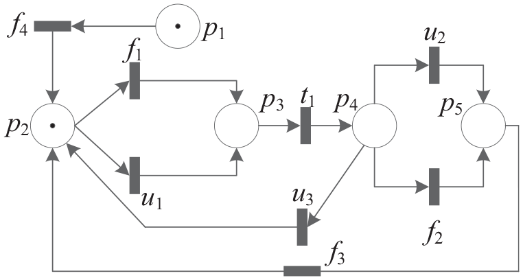
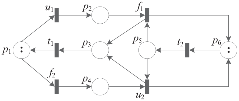
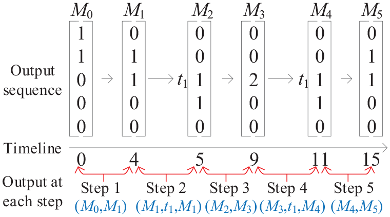
• Example 1. Consider the Petri net shown in Figure 1 , where $T_o=\{t_1\}$ , $T_u=\{f_1,f_2,f_3,f_4,u_1,u_2,u_3\}$ , and the initial marking is $M_0=p_1+p_2$ . If the time interval to read place sensors is four time units (i.e. $K=4$ ), then a possible evolution of the net is shown in Figure 2 . The timeline shows the moments to read place sensors. The output sequence obtained along this timeline is represented as a marking-transition sequence, that is, $M_0{M}_1{t}_1{M}_2{M}_3{t}_1{M}_4{M}_5$ , which contains five steps $(M_0,M_1),(M_1,t_2,M_2),(M_2,M_3),(M_3,t_1,M_4)$ and $(M_4,M_5)$ , as shown in the lower part of Figure 2.

Figure 1.

A Petri net for Example 1.

Figure 2.

A possible output sequence of the net in Figure 1.

In Step 1, from the starting point $M_0$ , no observable transition is observed during four time units. Then, at the fourth time unit, place sensors are read and the marking $M_1=p_2+p_3$ is obtained. Thus, the output in Step 1 is the first case mentioned above, that is, a marking pair $(M_0,M_1)$ . In Step 2, a timer restarts from marking $M_1$ and we observe transition $t_1$ before four time units elapse. In addition, by reading place sensors, the reached marking after firing $t_1$ is $M_2=p_3+p_4$ . Thus, the output in Step 2 can be represented as the second cases defined previously, that is, a three tuple $(M_1,t_1,M_2)$ . The outputs in Steps 3–5 can be similarly explained and are illustrated in Figure 2. ∇

• Definition 2. A trace of a Petri net system $〈N,M_0〉$ with $T=T_o\cup T_u$ is a sequence $\sigma =M_0{b}_1{M}_1{b}_2{M}_2\dots b_L{M}_L$ such that there exist unobservable transition sequences ${\sigma }_{u_1},{\sigma }_{u_2},\dots ,{\sigma }_{u_L}\in T_u^{*}$ satisfying $M_0[{\sigma }_{u_1}{b}_1〉M_1\dots {\sigma }_{u_L}{b}_L〉M_L$ , where $L\ge 1$ is a positive integer, $b_i\in T_o\cup \{\epsilon \}$ , $M_i\in R(N,M_0)$ , $i=1,\dots ,L.$ ∇

The set of traces of a net system $〈N,M_0〉$ is defined as $\mathcal{T}(N,M_0)=\left\{\sigma \right|\mathrm{is}\mathrm{a}\mathrm{trace}\}.$ Obviously, the output sequence of a Petri net in this paper, defined under Assumptions (A1) and (A2), is a trace. For example, the output sequence, say ${\sigma }_1$ , in Example 1 is a trace and it holds ${\sigma }_1\in \mathcal{T}(N,M_0)$ . Now, we are ready to formally define the fault diagnosis problem addressed in this paper.

• Problem 1. Given a Petri net system $〈N,M_0〉$ and a partition ${\Pi }_f=\{T_f^1,\dots ,T_f^r\}$ of $r$ fault classes, the problem consists in determining the occurrence of each fault class $T_f^i$ ( $i=1,\dots ,r$ ) till observing a trace $\sigma =M_0{b}_1{M}_1{b}_2{M}_2\dots b_L{M}_L$ that contains multiple steps with each being in the form of a marking pair $(M,M\prime )$ or a three tuple $(M,t_o,M\prime ).$

Fault diagnosis algorithm for Petri nets

In this section, we define a local diagnoser and a global diagnoser for solving Problem 1 and develop a fault diagnosis algorithm based on integer linear programing techniques. To formally present the algorithm, several new definitions are first provided.

• Definition 3. Given a net system $〈N,M_0〉$ with $T=T_o\cup T_u$ and two markings $M,M\prime \in R(N,M_0)$ , the set of unobservable transition sequences whose firings bring the system from $M$ to $M\prime$ is defined by $\Lambda (M,M\prime )=\{{\sigma }_u\in T_u^{*}|M[{\sigma }_u〉M\prime \}.$ ∇

It is clear that if $M\prime$ is reachable from $M$ by firing a sequence ${\sigma }_u\in T_u^{*}$ , that is, $M[{\sigma }_u〉M\prime$ , then $\Lambda (M,M\prime )\ne \varnothing .$ When observing a pair $(M,M\prime )$ during the evolution of a step of a system, the following local diagnoser describes the diagnosis decision of each fault class $T_f^i\in {\Pi }_f$ after observing $(M,M\prime ).$

• Definition 4. A local diagnoser is a function $\mathrm{\Delta }:{\mathbb{N}}^m\times {\mathbb{N}}^m\times {\Pi }_f\to \{0,1,2\}$ which associates a pair $(M,M\prime )$ and each fault class $T_f^i\in {\Pi }_f$ with a diagnosis state such that

• • $\mathrm{\Delta }(M,M\prime ,T_f^i)=0$ if for all $f\in T_f^i$ and for all ${\sigma }_u\in \Lambda (M,M\prime )$ it holds $f\notin {\sigma }_u$ , that is, there are multiple paths from $M$ to $M\prime$ in the reachability graph but each path does not contain transition $f$ . In such a case, the system behaves normally between $M$ and $M\prime$ and no fault occurs.

• • $\mathrm{\Delta }(M,M\prime ,T_f^i)=1$ if there exist two unobservable transition sequences ${\sigma }_{u_1},{\sigma }_{u_2}\in \Lambda (M,M\prime )$ such that (i) there exists a fault $f\in T_f^i$ satisfying $f\in {\sigma }_{u_1}$ , and (ii) for all $f\in T_f^i$ , it holds $f\notin {\sigma }_{u_2}$ , that is, there are at least two possible paths from $M$ to $M\prime$ in the reachability graph, one passing a fault $f\in T_f^i$ but another passing none of them.

• • $\mathrm{\Delta }(M,M\prime ,T_f^i)=2$ if for all ${\sigma }_u\in \Lambda (M,M\prime )$ there exists a fault $f\in T_f^i$ satisfying $f\in {\sigma }_u$ , that is, each path from $M$ to $M\prime$ in the reachability graph contains a fault $f\in T_f^i.$ ∇

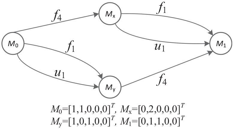
• Example 2. By specifying $T_f^1=\{f_1,f_4\}$ and $T_f^2=\{f_2,f_3\}$ , let us consider the Petri net shown in Figure 1again. Consider two markings $M_0=p_1+p_2$ and $M_1=p_2+p_3$ as shown in Figure 2. Figure 3is a part of the reachability graph, describing all possible paths from $M_0$ to $M_1$ that contain unobservable transitions only.

Figure 3.

A part of the reachability graph of the net in Figure 1.

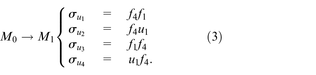
It is easy to verify that there are four paths from $M_0$ to $M_1$ , as shown in the following:

$$M_0\to M_1\{\begin{array}{ccc}{\sigma }_{u_1}\hfill & =\hfill & f_4{f}_1\hfill \\ \multicolumn{1}{c}{{\sigma }_{u_2}}& =\hfill & f_4{u}_1\hfill \\ \multicolumn{1}{c}{{\sigma }_{u_3}}& =\hfill & f_1{f}_4\hfill \\ \multicolumn{1}{c}{{\sigma }_{u_4}}& =\hfill & u_1{f}_4.\hfill \end{array}$$

(3)

Since $f_4\in T_f^1$ is contained in ${\sigma }_{u_1},{\sigma }_{u_2},{\sigma }_{u_3},$ and ${\sigma }_{u_4}$ , it holds $\mathrm{\Delta }(M_0,M_1,T_f^1)=2$ according to Def. 4. Following a similar reasoning, the diagnosis decision $\mathrm{\Delta }(M_0,M_1,T_f^2)=0$ is obtained. ∇

It is not realistic to compute diagnosis decision of each fault class via reachability graph analysis because of the state explosion problem. we next provide a linear algebraic characterization of all possible unobservable transition sequences from one marking to another.

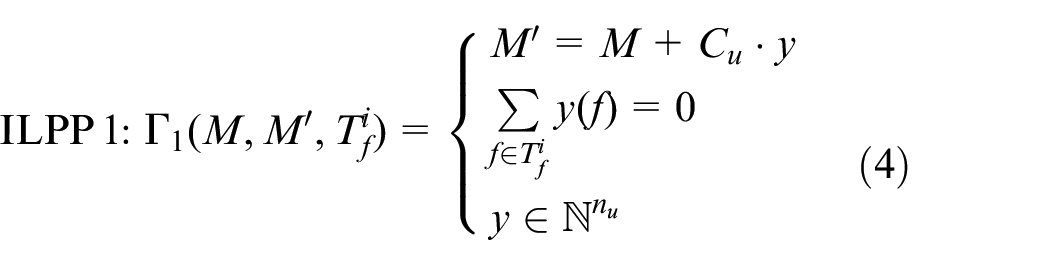
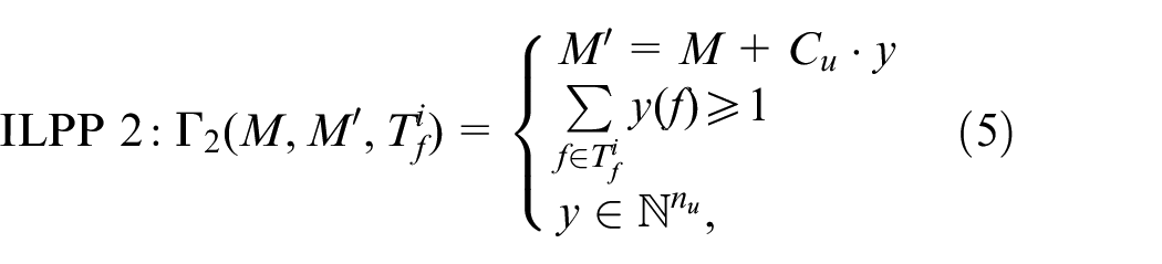
For two markings $M,M\prime \in R(N,M_0)$ and a fault class $T_f^i\in {\Pi }_f$ , we construct the following two ILP problems

$$\begin{array}{c}\mathrm{ILPP}1:{\mathrm{\Gamma }}_1(M,M\prime ,T_f^i)=\{\begin{array}{c}M\prime =M+C_u·y\hfill \\ \multicolumn{1}{c}{\sum _{f\in T_f^i}y(f)=0}\\ \multicolumn{1}{c}{y\in {\mathbb{N}}^{n_u}}\end{array}\hfill \end{array}$$

(4)

$$\mathrm{ILPP}2:{\mathrm{\Gamma }}_2(M,M\prime ,T_f^i)=\{\begin{array}{c}M\prime =M+C_u·y\hfill \\ \multicolumn{1}{c}{\sum _{f\in T_f^i}y(f)\ge 1}\\ \multicolumn{1}{c}{y\in {\mathbb{N}}^{n_u},}\end{array}$$

(5)

where $y$ is a non-negative integer vector of $n_u$ -dimension. The item $\sum _{f\in T_f^i}y(f)$ stands for the sum of components of $y$ corresponding to all fault transitions in $T_f^i$ . On the basis of these two ILP problems, we obtain the following theorem:

• Theorem 2. Let $〈N,M_0〉$ be a Petri net system with $T=T_o\cup T_u$ and $T_f=T_f^1\cup \dots \cup T_f^r\subseteq T_u.$ For two markings $M,M\prime \in R(N,M_0)$ with $M\prime$ being reachable from $M$ by firing an unobservable transition sequence, and a fault class $T_f^i\in {\Pi }_f$ , it holds

• (1)  $\mathrm{\Delta }(M,M\prime ,T_f^i)=2$ if and only if ILPP 1 has no feasible solution,

• (2)  $\mathrm{\Delta }(M,M\prime ,T_f^i)=0$ if and only if ILPP 2 has no feasible solution,

• (3)  $\mathrm{\Delta }(M,M\prime ,T_f^i)=1$ if and only if both ILPP 1 and ILPP 2 admit a solution,

Proof. We prove the results (1)–(3) in turn.

• (1): (if) Since $M\prime$ is reachable from $M$ by firing an unobservable transition sequence, there necessarily exists a column vector $y$ satisfying $M\prime =M+C_u·y$ . On the other hand, if ILPP 1 has no feasible solution, then there does not exist an unobservable transition sequence that contains none of fault transitions in $f\in T_f^i$ and whose firing brings the system from $M$ to $M\prime$ , that is, for all ${\sigma }_u\in \Lambda (M,M\prime )$ , $T_f^i\in {\sigma }_u$ . According to Def. 4, we have $\mathrm{\Delta }(M,M\prime ,T_f^i)=2$ . (only if) If ILPP 1 admits a solution, there exists a sequence ${\sigma }_u\in T_u^{*}$ such that $M[{\sigma }_u〉M\prime$ and $T_f^i\notin {\sigma }_u$ according to Theorem 1. Namely, it holds $\mathrm{\Delta }(M,M\prime ,T_f^i)=1$ or $0$ . Clearly, this violates the condition $\mathrm{\Delta }(M,M\prime ,T_f^i)=2$ . Thus, this result is proved by contradiction.

• (2): (if ) If ILPP 2 has no feasible solution, all possible unobservable transition sequences from $M$ to $M\prime$ in the reachability graph do not pass one of fault transition $f\in T_f^i$ , that is, for all ${\sigma }_u\in \Lambda (M,M\prime )$ , $T_f^i\notin {\sigma }_u$ . Thus, we conclude $\mathrm{\Delta }(M,M\prime ,T_f^i)=0$ by Def. 4. (only if) We prove this result by contradiction. If ILPP 2 has a solution, by Theorem 1, there is a sequence ${\sigma }_u$ satisfying $M[{\sigma }_u〉M\prime$ and $T_f^i{\sigma }_u$ , that is, $\mathrm{\Delta }(M,M\prime ,T_f^i)\ne 0$ . This violates the condition $\mathrm{\Delta }(M,M\prime ,T_f^i)=0$ .

• (3): (if ) If both ILPP 1 and ILPP 2 have a solution, by Theorem 1, there exist two sequence ${\sigma }_{u_1},{\sigma }_{u_2}$ such that $T_f^i\notin {\sigma }_{u_1}$ and $T_f^i\in {\sigma }_{u_2}$ . Thus, it holds $\mathrm{\Delta }(M,M\prime ,T_f^i)=1$ by Def. 4. (only if) By contradiction, we first assume that ILPP 1 has no solution. Then, we have $\mathrm{\Delta }(M,M\prime ,T_f^i)=2$ according to the result (1). This violates the condition $\mathrm{\Delta }(M,M\prime ,T_f^i)=1$ . Thus, ILPP 1 necessarily has a solution. If we assume that ILPP 1 has no solution, it holds $\mathrm{\Delta }(M,M\prime ,T_f^i)=0$ according to the result (2). This violates $\mathrm{\Delta }(M,M\prime ,T_f^i)=1$ . Thus, we prove that both ILPP1 and ILPP1 admit a solution. □

Given two markings $M,M\prime \in R(N,M_0)$ and a fault class $T_f^i\in {\Pi }_f$ , the local diagnoser $\mathrm{\Delta }(M,M\prime ,T_f^i)$ can be computed by solving ILPPs 1 and 2 according to Theorem 2. However, the final aim of fault diagnosis is to determine the occurrence of faults till observing a trace $\sigma =M_0{b}_1{M}_1{b}_2{M}_2\dots b_L{M}_L$ , as described in Problem 1. Thus, we provide the following definitions to achieve the aim.

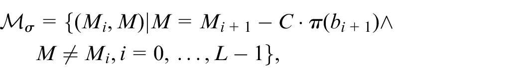
• Definition 5. Given a trace $\sigma =M_0{b}_1{M}_1{b}_2{M}_2\dots b_L{M}_L\in \mathcal{T}(N,M_0)$ of a net system $〈N,M_0〉$ , the set of its associated marking pairs is define as

$$\begin{array}{c}\multicolumn{1}{c}{{\mathcal{M}}_{\sigma }=\{(M_i,M)|M=M_{i+1}-C·\mathrm{\pi }(b_{i+1})\wedge }\\ M\ne M_i,i=0,\dots ,L-1\},\hfill \end{array}$$

where $\mathrm{\pi }(b_i)={\overrightarrow{0}}^n$ if $e_i=\epsilon .$ ∇

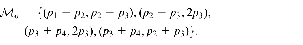
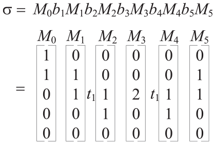
• Example 3. Consider the net shown in Figure 1 and one of its traces $\sigma =M_0{b}_1{M}_1{b}_2{M}_2{b}_3{M}_3{b}_4{M}_4{b}_5{M}_5$ , as shown in Figure 4 . In this trace, we have $b_1=b_3=b_5=\epsilon$ and $b_2=b_4=t_1$ . In addition, it is clear that $C·\mathrm{\pi }(t_1)=[00-110{]}^T$ . Thus, by Def. 5, it holds

$$\begin{array}{c}{\mathcal{M}}_{\sigma }=\{(p_1+p_2,p_2+p_3),(p_2+p_3,2p_3),\hfill \\ (p_3+p_4,2p_3),(p_3+p_4,p_2+p_3)\}.\hfill \end{array}$$

Figure 4.

A trace of the net in Figure 1.

When computing the set ${\mathcal{M}}_{\sigma }$ , we delete a marking pair $(2p_3,2p_3)$ since $2p_3=2p_3$ (i.e. $M=M_i$ ).

• Definition 6. A global diagnoser of a net $〈N,M_0〉$ is a function $\mathrm{\Theta }:T(N,M_0)\times {\Pi }_f\to \{0,1,2\}$ that associates a trace $\sigma \in \mathcal{T}(N,M_0)$ and a fault class $T_f^i\in {\Pi }_f$ with a diagnosis decision such that

• • $\mathrm{\Theta }(\sigma ,T_f^i)=0$ if for all pairs $(M,M\prime )\in {\mathcal{M}}_{\sigma }$ , it holds $\mathrm{\Delta }(M,M\prime ,T_f^i)=0$ ,

• • $\mathrm{\Theta }(\sigma ,T_f^i)=1$ if (i) there exists a pair $(M,M\prime )\in {\mathcal{M}}_{\sigma }$ such that $\mathrm{\Delta }(M,M\prime ,T_f^i)=1$ and (ii) there does not exist a pair $(M,M\prime )\in {\mathcal{M}}_{\sigma }$ such that $\mathrm{\Delta }(M,M\prime ,T_f^i)=2$ ,

• • $\mathrm{\Theta }(\sigma ,T_f^i)=2$ if there exists a pair $(M,M\prime )\in {\mathcal{M}}_{\sigma }$ such that $\mathrm{\Delta }(M,M\prime ,T_f^i)=2.$ ∇

In plain terms, the diagnosis decision $\mathrm{\Theta }(\sigma ,T_f^i)=0$ means that the fault class $T_f^i$ does not occur during each step of the trace $\sigma$ . The decision $\mathrm{\Theta }(\sigma ,T_f^i)=2$ implies that $T_f^i$ necessarily has occurred in one of steps of $\sigma$ . Consequently, all paths from $M_0$ to $M_L$ in the reachability graph include the transitions in the step and necessarily pass a fault transition $f\in T_f^i$ .

In Def. 6, we observe that the global diagnoser of a trace $\sigma$ can be computed by inspecting all local diagnosers of steps in the trace. Next, we develop an algorithm to detect faults that have occurred till the observation of a trace.

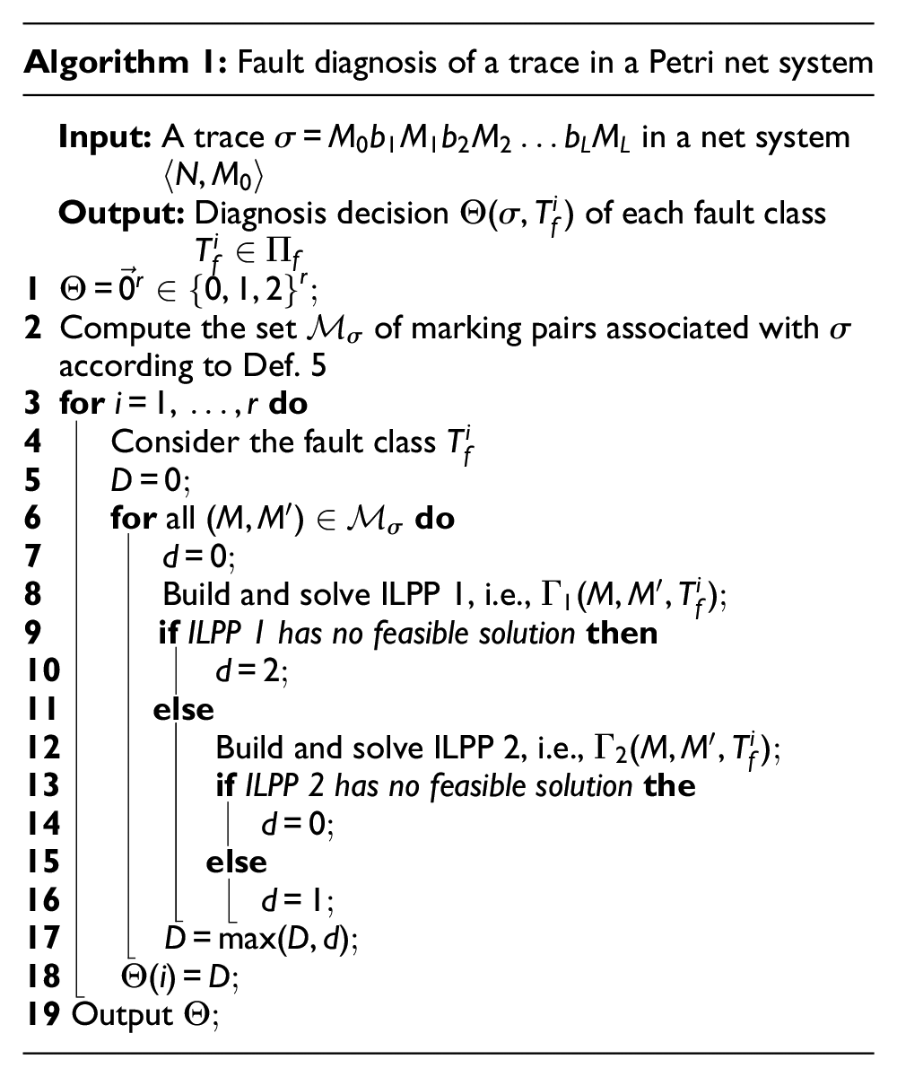
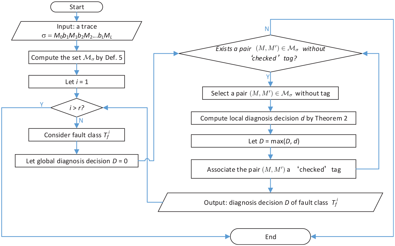
The main logical flow of Algorithm 1 is illustrated by the flowchart shown in Figure 5. More specifically, in Line 1, the global diagnoser $\mathrm{\Theta }$ is initialized to an $r$ -dimensional column vector $\mathrm{\Theta }={\overrightarrow{0}}^r\in \{0,1,2{\}}^r$ such that $\mathrm{\Theta }(i)$ stands for the diagnosis decision of fault class $T_f^i$ , where $r$ is the number of fault classes and 0, 1, and 2 are the diagnosis decisions. We compute the diagnosis decisions of all fault classes in turn, as shown in Line 3. For a fault class $T_f^i$ , the fault decision $\mathrm{\Theta }(i)$ is computed in Lines 5–18. The variable $D=0$ in Line 1 represents the global diagnosis decision and $d=0$ in Line 7 denotes a local decision. For all marking pairs $(M,M\prime )\in {\mathcal{M}}_{\sigma }$ , the local diagnosis decision $d$ is obtained by solving ILPP 1 and/or ILPP 2. The global diagnosis decision is computed by selecting the maximal local decision of all marking pairs, as shown in Line 17.

Algorithm 1: Fault diagnosis of a trace in a Petri net system

Input: A trace $\sigma =M_0{b}_1{M}_1{b}_2{M}_2\dots b_L{M}_L$ in a net system $〈N,M_0〉$  Output: Diagnosis decision $\mathrm{\Theta }(\sigma ,T_f^i)$ of each fault class $T_f^i\in {\Pi }_f$ 1  $\mathrm{\Theta }={\overrightarrow{0}}^r\in \{0,1,2{\}}^r;$ 2 Compute the set ${\mathcal{M}}_{\sigma }$ of marking pairs associated with $\sigma$ according to Def. 5 3 for $i=1,\dots ,r$ do 4  Consider the fault class $T_f^i$ 5   $D=0;$ 6  for all $(M,M\prime )\in {\mathcal{M}}_{\sigma }$ do 7     $d=0;$ 8    Build and solve ILPP 1, i.e., ${\mathrm{\Gamma }}_1(M,M\prime ,T_f^i);$ 9      ifILPP 1 has no feasible solution then 10      $d=2;$ 11     else 12     Build and solve ILPP 2, i.e., ${\mathrm{\Gamma }}_2(M,M\prime ,T_f^i);$ 13     ifILPP 2 has no feasible solution the 14       $d=0;$ 15        else 16            $d=1;$ 17      $D=\max (D,d);$ 18    $\mathrm{\Theta }(i)=D;$ 19 Output $\mathrm{\Theta };$

Figure 5.

The flowchart of Algorithm 1.

The main computational cost of Algorithm 1 stems from the solution of ILPP 1 and/or ILPP 2. It is well known that the complexity of an integer linear programing problem is NP-complete and is closely related to its size (i.e. the numbers of unknown variables and constraints). However, in practice, many integer linear programing problems can be efficiently solved using commercial solvers (such as Gurobi Solver ⁴⁶ used in the paper). Since integer linear programing problems ILPP 1 and ILPP 2 have the same size, we analyze the size of ILPP 1 only. The number of unknown variables is denoted by

$$\mathcal{I}=n_u,$$

(6)

where $n_u$ is the number of unobservable transitions; the number of constraints is denoted by

$$\mathcal{J}=m+1,$$

(7)

where $m$ is the cardinality of place set. We observe that the size of ILPP 1 is regardless of the length $L$ of a trace $\sigma$ .

• Proposition 1. Given a trace $\sigma =M_0{b}_1{M}_1{b}_2{M}_2\dots b_L{M}_L$ of a net system $〈N,M_0〉$ , for all fault classes $T_f^i\in {\Pi }_f$ , Algorithm 6 outputs the correct diagnosis decision $\mathrm{\Theta }(\sigma ,T_f^i)$ .

Proof. According to Theorem 2, the local diagnosis decision $\mathrm{\Delta }(M,M\prime ,T_f^i)$ of each marking pair $(M,M\prime )\in {\mathcal{M}}_{\sigma }$ is correctly computed in Lines 6–16. We next prove that it is correct to compute the global diagnosis decision by selecting the maximal local diagnosis decision, that is, $D=\max (D,d)$ in Line 17. If for all $(M,M\prime )\in {\mathcal{M}}_{\sigma }$ , we have $\mathrm{\Delta }(M,M\prime ,T_f^i)=0$ , that is, $d=0$ , then the algorithm outputs $D=\mathrm{\Theta }(\sigma ,T_f^i)=0$ . This is obviously correct according to Def. 6. On the other hand, if there exists a pair $(M,M\prime )\in {\mathcal{M}}_{\sigma }$ with $d=\mathrm{\Delta }(M,M\prime ,T_f^i)=1$ and there does not exist a pair $(\overline{M},\overline{M}\prime )$ with $\mathrm{\Delta }(\overline{M},\overline{M}\prime ,T_f^i)=2$ , the maximal value will be 1,that is, $D=\max (D,d)=1$ . This result can be readily verified by Def. 6. Finally, if there exists a pair $(M,M\prime )\in {\mathcal{M}}_{\sigma }$ with $d=\mathrm{\Delta }(M,M\prime ,T_f^i)=2$ , it is clear that $D=\max (D,d)=2$ . This is also consistent with Def. 6. □

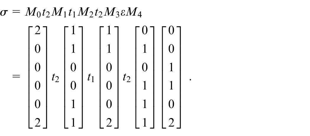
• Example 4. Let us consider the net system shown in Figure 6 , where $T_o=\{t_1,t_2\}$ , $T_u=\{u_1,u_2,f_1,f_2\}$ , $T_f^1=\{f_1\}$ , and $T_f^2=\{f_2\}$ . Assume that one of the traces of the net is

$$\begin{array}{c}\multicolumn{1}{c}{\sigma =M_0{t}_2{M}_1{t}_1{M}_2{t}_2{M}_3\epsilon M_4}\\ =\left[\begin{array}{c}2\hfill \\ \multicolumn{1}{c}{0}\\ \multicolumn{1}{c}{0}\\ \multicolumn{1}{c}{0}\\ \multicolumn{1}{c}{0}\\ \multicolumn{1}{c}{2}\end{array}\right]t_2\left[\begin{array}{c}1\hfill \\ \multicolumn{1}{c}{1}\\ \multicolumn{1}{c}{0}\\ \multicolumn{1}{c}{0}\\ \multicolumn{1}{c}{1}\\ \multicolumn{1}{c}{1}\end{array}\right]t_1\left[\begin{array}{c}1\hfill \\ \multicolumn{1}{c}{1}\\ \multicolumn{1}{c}{0}\\ \multicolumn{1}{c}{0}\\ \multicolumn{1}{c}{0}\\ \multicolumn{1}{c}{2}\end{array}\right]t_2\left[\begin{array}{c}0\hfill \\ \multicolumn{1}{c}{1}\\ \multicolumn{1}{c}{0}\\ \multicolumn{1}{c}{1}\\ \multicolumn{1}{c}{1}\\ \multicolumn{1}{c}{1}\end{array}\right]\left[\begin{array}{c}0\hfill \\ \multicolumn{1}{c}{0}\\ \multicolumn{1}{c}{1}\\ \multicolumn{1}{c}{1}\\ \multicolumn{1}{c}{0}\\ \multicolumn{1}{c}{2}\end{array}\right].\hfill \end{array}$$

Figure 6.

A Petri net for Example 4.

We compute the global diagnoser $\mathrm{\Theta }(\sigma ,T_f^1)$ and $\mathrm{\Theta }(\sigma ,T_f^2)$ using Algorithm 1. The global diagnosis decisions are represented as a two-dimensional column vector $\mathrm{\Theta }$ such that $\mathrm{\Theta }(1)=\mathrm{\Theta }(\sigma ,T_f^1)$ and $\mathrm{\Theta }(2)=\mathrm{\Theta }(\sigma ,T_f^2)$ . At first, $\mathrm{\Theta }$ is set to $\mathrm{\Theta }=[00{]}^T$ . According to Def. 5, we have ${\mathcal{M}}_{\sigma }=\{{\mathcal{P}}_1,{\mathcal{P}}_2,{\mathcal{P}}_3,{\mathcal{P}}_4\}=\{(2p_1+2p_6,p_1+p_2+2p_6)$ , $(p_1+p_2+p_5+p_6,p_2+p_3+2p_6),$ $(p_1+p_2+2p_6,p_2+p_4+2p_6)$ , $(p_2+p_4+p_5+p_6,p_3+p_4+2p_6)\}.$

For the pair ${\mathcal{P}}_1\in {\mathcal{M}}_{\sigma }$ , the local diagnosis decision for $T_f^1$ is $d=0$ by Lines 7–16. The global diagnosis decision of $T_f^1$ is updated by $\mathrm{\Theta }(1)=\max (\mathrm{\Theta }(1),d)=0$ . Using the same reasoning, we have $\mathrm{\Theta }(2)=\max (\mathrm{\Theta }(2),0)=0$ . For the pair ${\mathcal{P}}_2\in {\mathcal{M}}_{\sigma }$ , we have $\mathrm{\Theta }(1)=\max (\mathrm{\Theta }(1),1)=1$ and $\mathrm{\Theta }(2)=\max (\mathrm{\Theta }(2),1)=1$ . Analogously, for ${\mathcal{P}}_3$ , the local diagnosis decision is $\overrightarrow{d}=[\mathrm{\Delta }(M,M\prime ,T_f^1)\mathrm{\Delta }(M,M\prime ,T_f^2){]}^T=[12{]}^T$ and the global diagnosis decision is updated by $\mathrm{\Theta }=[\max (\mathrm{\Theta }(1),1)\max (\mathrm{\Theta }(2),2){]}^T=[12{]}^T$ . Finally, for ${\mathcal{P}}_4$ , we have $\overrightarrow{d}=[22{]}^T$ and $\mathrm{\Theta }=[\max (\mathrm{\Theta }(1),2)\max (\mathrm{\Theta }(2),2){]}^T=[22{]}^T.$ ∇

Fault diagnosis algorithm for LPNs

This section extends the fault diagnosis algorithm for Petri nets to the case of labeled Petri nets. In LPNs, two or more observable transitions may share the same label and an observation often corresponds to multiple traces of the underlying Petri nets. Thus, the algorithm for LPNs needs to enumerate all possible transitions with the same label and combine diagnosis results for different traces.

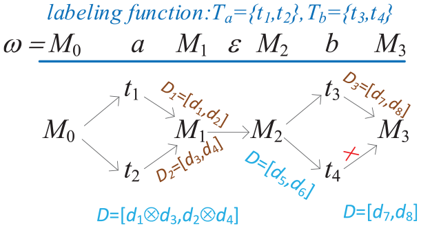
• Definition 7. A labeled trace of an LPN system $〈N,M_0,E,\lambda 〉$ is a sequence $\omega =M_0{e}_1{M}_1{e}_2{M}_2\dots e_L{M}_L$ such that there exists a trace $\sigma =M_0{b}_1{M}_1{b}_2{M}_2\dots b_L{M}_L\in \mathcal{T}(N,M_0)$ , where $L\ge 1$ is a positive integer, $e_i\in E\cup \{\epsilon \},b_i\in T_{e_i}\cup \{\epsilon \},$ and $M_i\in R(N,M_0),i=1,\dots ,L.$ ∇

In plain words, if we observe a labeled trace $\omega$ , the underlying evolution of a system is a trace $\sigma$ such that $\lambda (b_i)=e_i$ with $i=1,\dots ,L$ . We use $e_i{M}_i\in \omega$ to denote that $e_i{M}_i$ is contained in $\omega$ , $i\in \{1,\dots ,L\}$ . To conveniently present the fault diagnosis algorithm for LPNs, we define the following operator.

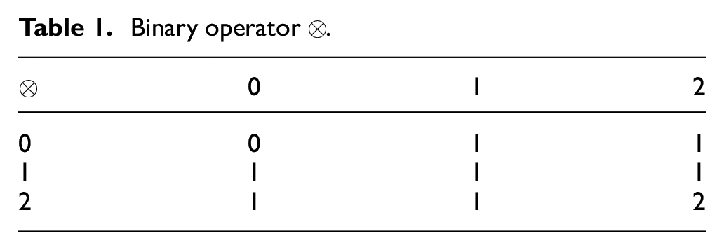
• Definition 8. The operator $\otimes :\{0,1,2\}\times \{0,1,2\}\to \{0,1,2\}$ associates two operands $a,b\in \{0,1,2\}$ with a value $c\in \{0,1,2\}$ according to Table 1, which is written as $a\otimes b=c$ .

Table 1.

Binary operator ⊗.

⊗	0	1	2
0	0	1	1
1	1	1	1
2	1	1	2

Given a labeled trace $\omega$ , there often exist multiple traces $\sigma$ ’s that have the same observation. We use the operator ⊗ to combine the diagnosis decisions of these traces to form the diagnosis result of the labeled trace. Algorithm 2 illustrates the usage of ⊗. Before present the algorithm, we define an ILP problem:

$$\mathrm{\Gamma }(M,M\prime )=\{\begin{array}{c}M\prime =M+C_u·y\hfill \\ \multicolumn{1}{c}{y\in {\mathbb{N}}^{n_u},}\end{array}$$

(8)

which characterizes if there exists an unobservable transition sequence ${\sigma }_u$ such that $M[{\sigma }_u〉M\prime$ and $y=\mathrm{\pi }({\sigma }_u)$ . If $\mathrm{\Gamma }(M,M\prime )$ admits a solution, there necessarily exists such a sequence by Theorem 1. Otherwise, such a sequence does not exist. Now, it is ready to present the fault diagnosis algorithm for LPNs.

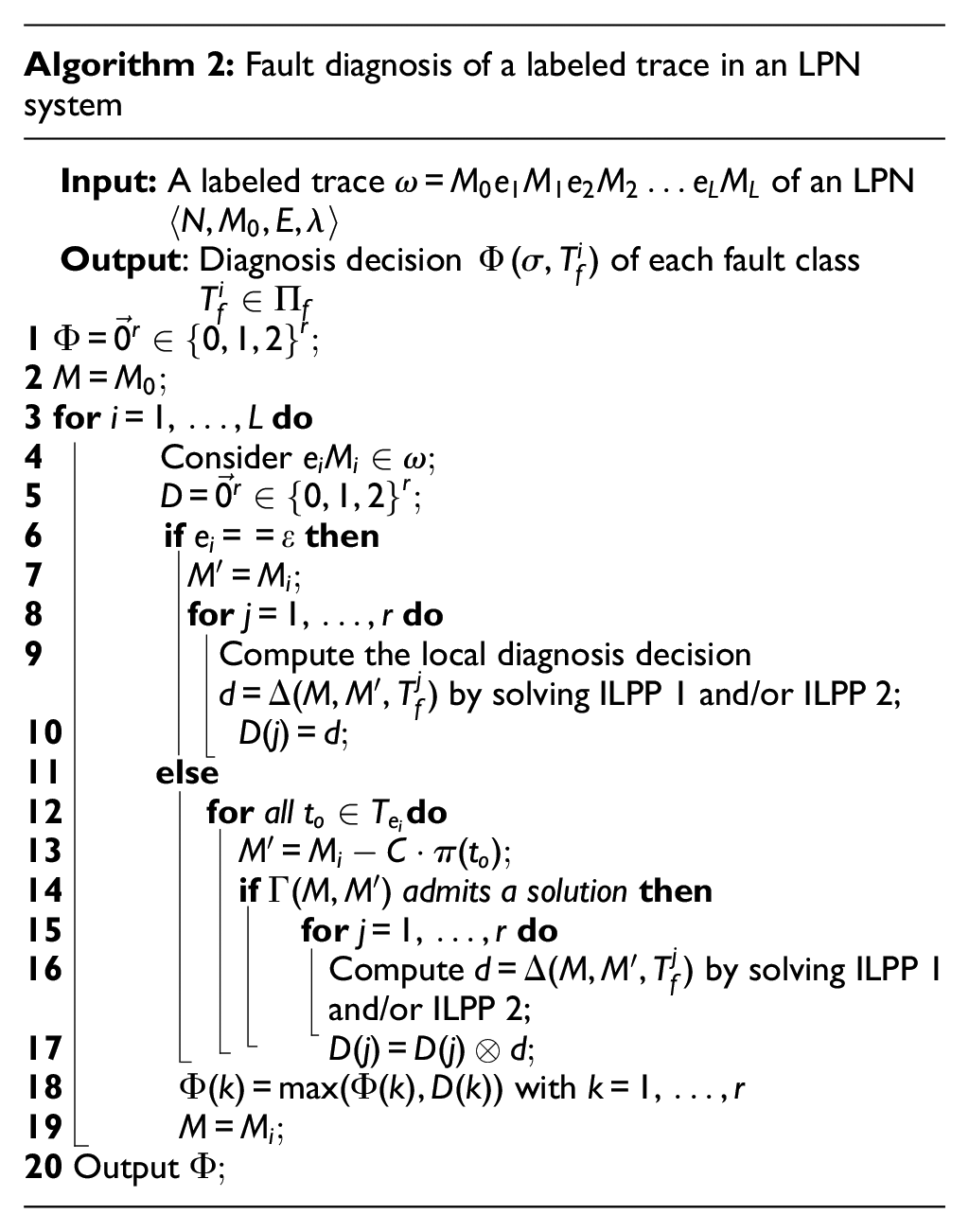
Algorithm 2: Fault diagnosis of a labeled trace in an LPN system

Input: A labeled trace $\omega =M_0{e}_1{M}_1{e}_2{M}_2\dots e_L{M}_L$ of an LPN $〈N,M_0,E,\lambda 〉$  Output: Diagnosis decision $\Phi (\sigma ,T_f^i)$ of each fault class $T_f^i\in {\Pi }_f$ 1 $\Phi ={\overrightarrow{0}}^r\in \{0,1,2{\}}^r;$ 2 $M=M_0;$ 3 for $i=1,\dots ,L$ do 4  Consider $e_i{M}_i\in \omega ;$ 5  $D={\overrightarrow{0}}^r\in \{0,1,2{\}}^r;$ 6  if $e_i==\epsilon$ then 7   $M\prime =M_i;$ 8 for   $j=1,\dots ,r$ do 9    Compute the local diagnosis decision $d=\mathrm{\Delta }(M,M\prime ,T_f^j)$ by solving ILPP 1 and/or ILPP 2; 10    $D(j)=d;$ 11   else 12    forall $t_o\in T_{e_i}$ do 13     $M\prime =M_i-C·\mathrm{\pi }(t_o);$ 14     if $\mathrm{\Gamma }(M,M\prime )$ admits a solution then 15      for $j=1,\dots ,r$ do 16       Compute $d=\mathrm{\Delta }(M,M\prime ,T_f^j)$ by solving ILPP 1 and/or ILPP 2; 17       $D(j)=D(j)\otimes d;$ 18    $\Phi (k)=\max (\Phi (k),D(k))$ with $k=1,\dots ,r$ 19    $M=M_i;$ 20 Output $\Phi ;$

In Algorithm 2, the global diagnosis decisions of a labeled trace $\omega$ are stored in an $r$ -dimensional vector $\Phi$ , as shown in Line 1. All steps $e_i{M}_i\in \omega$ ( $i=1,\dots ,L$ ) are considered in turn in Line 3. For each $e_i{M}_i$ , the local diagnosis decisions are recorded in $D={\overrightarrow{0}}^r\in \{0,1,2{\}}^r$ . If $e_i$ is the empty string in Line 6, we compute the diagnosis decision $d=\mathrm{\Delta }(M,M\prime ,T_f^j)$ of each fault class $T_f^j$ by solving ILPP 1 and/or ILPP 2. Otherwise, we check all transitions $t_o$ ’s with label $e_i$ in Line 12 and update $M\prime$ by $M\prime =M_i-C·\mathrm{\pi }(t_o).$ If the programing $\mathrm{\Gamma }(M,M\prime )$ has a solution in Line 14, there necessarily exists an unobservable transition sequence ${\sigma }_u$ such that $M[{\sigma }_u〉M\prime [t_o〉M_i.$ Then, the diagnosis decision $d=\mathrm{\Delta }(M,M\prime ,T_f^j)$ can be computed by solving ILPPs 1 and 2 and the diagnosis decisions for different $t_o$ ’s are combined by the operator ⊗ in Line 17. Finally, the global diagnosis $\Phi$ are obtained by combine diagnosis vector $D$ ’s of all steps $(e_i{M}_i)$ ’s using the max operation in Line 18.

• Example 5. Let us consider an LPN $〈N,M_0,E,\lambda 〉$ with $T=T_o\cup T_u$ , $T_o=\{t_1,t_2,t_3,t_4\}$ , and $E=\{a,b\}$ . The labels of all unobservable transitions are the empty string and the labels of observable transitions are represented as $\lambda (t_1)=\lambda (t_2)=a$ and $\lambda (t_3)=\lambda (t_4)=b$ (i.e. $T_a=\{t_1,t_2\}$ and $T_b=\{t_3,t_4\}$ ). Given a labeled trace $\omega =M_{0}a{M}_1{M}_{2}b{M}_3$ , we show how Algorithm 2 works by taking $\omega$ as an input. The fault diagnosis process is illustrated by Figure 7.

Figure 7.

An example of fault diagnosis process of Algorithm 2.

For Step 1 “ $a{M}_1$ ” of $\omega$ , we consider $t_1,t_2\in T_a$ in turn, as shown in Line 12. In Figure 7 , for both $t_1$ and $t_2$ , $\mathrm{\Gamma }(M,M\prime )$ admits a solution. The corresponding diagnosis decisions are denoted by $D_1=[d_1,d_2]$ and $D_2=[d_3,d_4]$ , respectively. According to Line 17, the diagnosis decision vector $D$ for Step 1 is obtained by combining $D_1$ and $D_2$ using the operator ⊗, that is, $D=[d_1\otimes d_3,d_2\otimes d_4]$ , as shown in Figure 7 . For Step 2 “ $\epsilon M_2$ ,” the condition in Line 6 holds and the diagnosis vector in this step is represented by $D=[d_5,d_6]$ . Similar to Step 1, two observable transitions $t_3$ and $t_4$ with the same label $b$ in Step 3 “ $b{M}_3$ ” are inspected in turn. For $t_3\in T_b$ , the programing $\mathrm{\Gamma }(M,M\prime )$ has a solution. However, it has no feasible solution for $t_4\in T_b$ in Figure 7 . We mark this case with a symbol “×” in Figure 7 . Finally, the global diagnosis result vector $\Phi$ is obtained by combining all local diagnosis vectors of Steps 1–3 using max operation in Line 18. ∇

Case study

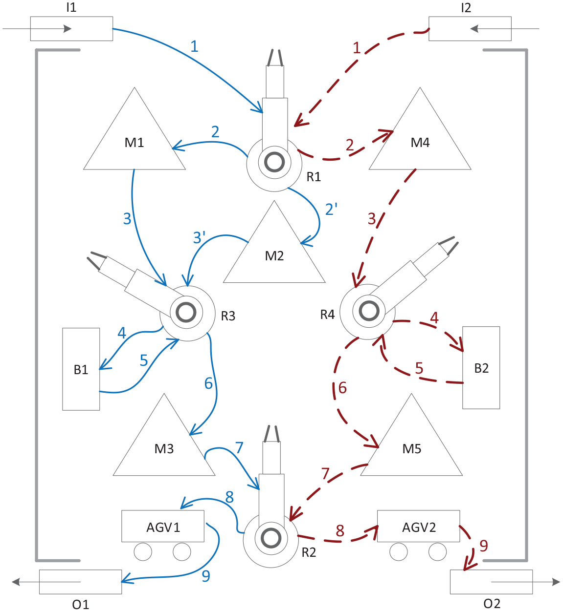
In this section, we show the application and computational efficiency of the proposed approach by means of a plant example. Let us consider the plant shown in Figure 8, which contains five machines (M1–M5), four robotic arms (R1–R4), two buffers with capacity 4 (B1 and B2), two entrances (I1 and I2), two exits (O1 and O2), and two automatic guided vehicles (AGV1 and AGV2).

Figure 8.

A plant including five machines and four robotic arms.

This plant has two production lines, as shown by the left part and right part of Figure 8, respectively:

• In production line 1 (i.e. the left part of Figure 8), robotic arm R1 first takes a raw part from entrance I1 and then load it into machine M1 or M2. After machine M1 or M2 finishes processing the part, robotic arm R3 unloads the part and puts it into buffer B1. When buffer B1 is not empty, R3 takes a part from B1 and loads it into machine M3. Robotic arm R2 unloads the finished part from M3 and puts it into AGV1 that transfers the part to exit O1.

• In production line 2 (i.e. the right part of Figure 8), robotic arm R1 takes a raw part from entrance I2 and loads it into machine M4. Robotic arm R4 unloads the processed part from M4 and puts it into buffer B2. When B2 is not empty, R4 takes a part from B2 and puts it into machine M5. Robotic arm R2 takes the finished part from M5 and puts it into AGV 2. Finally, the part is transferred to exit O2 by AGV 2.

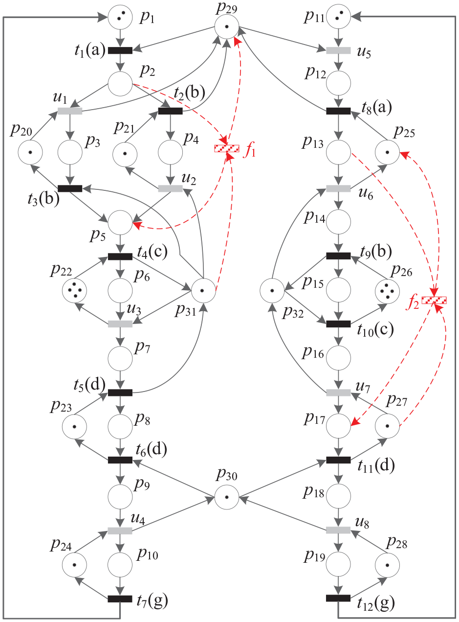
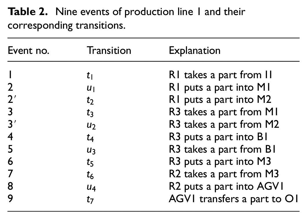
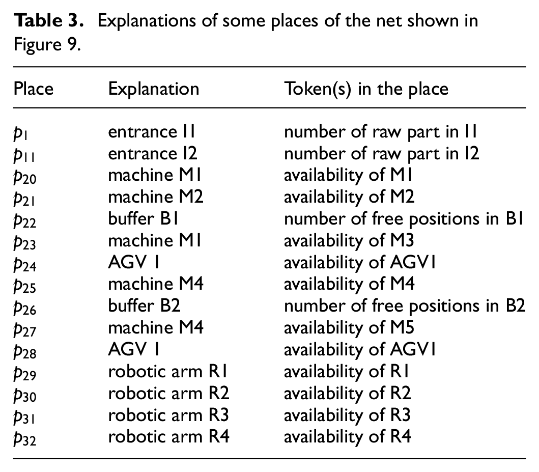
Each production line contains nine events, as indicated by the numbers 1–9 in Figure 8. The Petri net model of the plant is shown in Figure 9. Nine events of production line 1 and their corresponding transitions in Figure 9 are demonstrated in Table 2. The events of production line 2 and the corresponding transitions can be analogously explained. Apart from the events in each production line, the components (machines, robotic arms, etc.) of the plant shown in Figure 8 are also explicitly characterized by the places of the Petri net model shown in Figure 9, as listed in Table 3.

Figure 9.

A labeled Petri net model of an automated manufacturing system.

Table 2.

Nine events of production line 1 and their corresponding transitions.

Event no.	Transition	Explanation
1	$t_1$	R1 takes a part from I1
2	$u_1$	R1 puts a part into M1
2′	$t_2$	R1 puts a part into M2
3	$t_3$	R3 takes a part from M1
3′	$u_2$	R3 takes a part from M2
4	$t_4$	R3 puts a part into B1
5	$u_3$	R3 takes a part from B1
6	$t_5$	R3 puts a part into M3
7	$t_6$	R2 takes a part from M3
8	$u_4$	R2 puts a part into AGV1
9	$t_7$	AGV1 transfers a part to O1

Table 3.

Explanations of some places of the net shown in Figure 9.

Place	Explanation	Token(s) in the place
$p_1$	entrance I1	number of raw part in I1
$p_{11}$	entrance I2	number of raw part in I2
$p_{20}$	machine M1	availability of M1
$p_{21}$	machine M2	availability of M2
$p_{22}$	buffer B1	number of free positions in B1
$p_{23}$	machine M1	availability of M3
$p_{24}$	AGV 1	availability of AGV1
$p_{25}$	machine M4	availability of M4
$p_{26}$	buffer B2	number of free positions in B2
$p_{27}$	machine M4	availability of M5
$p_{28}$	AGV 1	availability of AGV1
$p_{29}$	robotic arm R1	availability of R1
$p_{30}$	robotic arm R2	availability of R2
$p_{31}$	robotic arm R3	availability of R3
$p_{32}$	robotic arm R4	availability of R4

We assume that there are two failures in the plant, which are described by two fault transitions $f_1$ and $f_2$ in Figure 9, respectively. Transition $f_1$ characterizes a failure that a part is stored into buffer B1 before being machined by machine M1 and $f_2$ describes that a part is directly processed by machine M5 before being stored into buffer B2.

The labeled Petri net model in Figure 9 has 32 places and 32 transitions, where $T_o=\{t_1,\dots ,t_{12}\},T_u=\{f_1,f_2,u_1,\dots ,u_8\},T_f^1=\{f_1\}$ , and $T_f^2=\{f_2\}$ . The initial marking is $M_0=2p_1+2p_{11}+p_{20}+p_{21}+4p_{22}+p_{23}+p_{24}+p_{25}+4p_{26}+p_{27}+p_{28}+p_{29}+p_{30}+p_{31}+p_{32}.$ Given an alphabet $E=\{a,b,c,d,g\}$ , the labels of the observable transitions are represented as $T_a=\{t_1,t_8\}$ , $T_b=\{t_2,t_3,t_9\}$ , $T_c=\{t_4,t_{10}\}$ , $T_d=\{t_5,t_6,t_{11}\}$ , and $T_g=\{t_7,t_{12}\}$ . In Figure 9, the label of each observable transition is demonstrated in parenthesis beside the transition.

In this case study, we compare the computational efficiency of the proposed approach with the ones in Fanti et al. ⁸ and Zhu et al. ²⁹  by following the steps below:

• Step 1: Simulate the operation of the net system shown in Figure 9 and generate an evolution, that is, a sequence that records all reached markings and fired transitions in order.

• Step 2: Compute three observations of the evolution generated in Step 1, which correspond to this paper Fanti et al. ⁸ and Zhu et al, ²⁹  respectively.

• Step 3: Run the diagnosis algorithms proposed in this paper,^8,29 respectively, by taking as input the corresponding observation, and record the running time at each step of the observation.

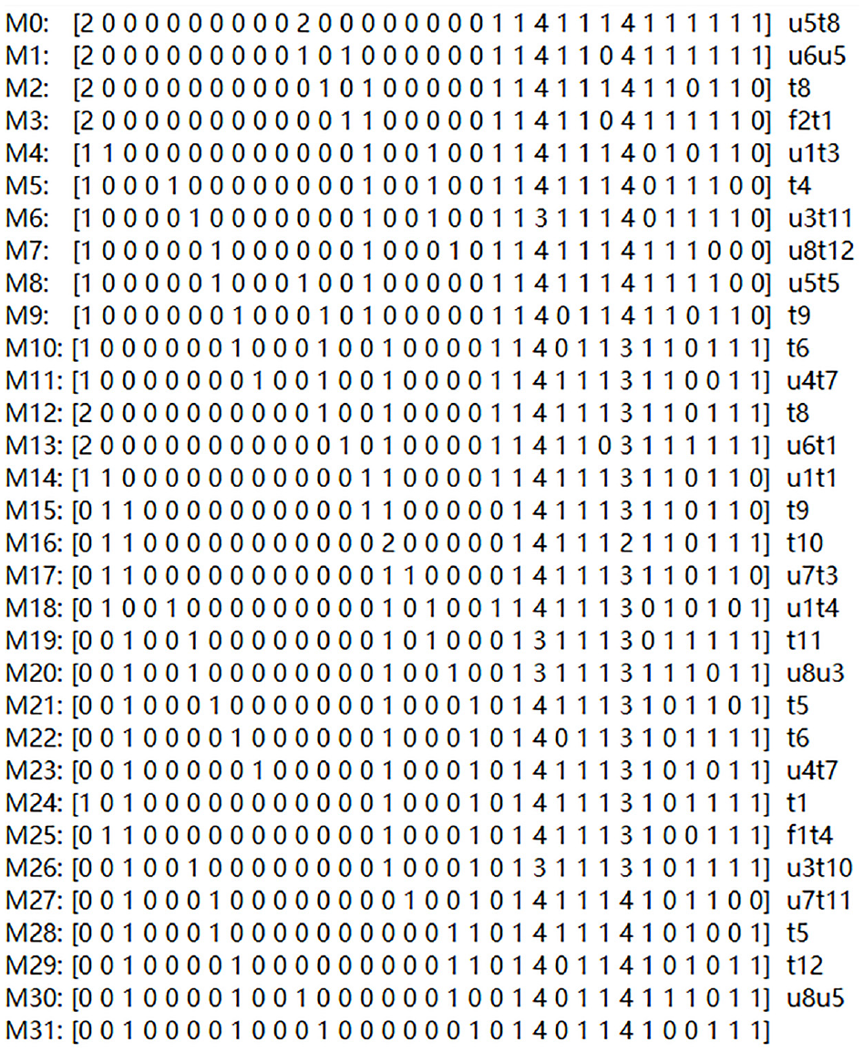
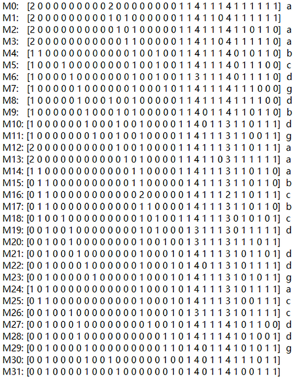
The generated evolution in Step 1 is shown in Figure 10. For this paper, the corresponding observation of the evolution is demonstrated in Figure 11, which is represented as ${\omega }_1=M_0{e}_1{M}_1{e}_2{M}_2\dots e_{31}{M}_{31}$ . Meanwhile, for the approaches in Fanti et al. ⁸ and Zhu et al., ²⁹  the observation of the evolution is ${\omega }_2=\mathrm{aaabcdgdbdgaaabcbcdddgaccddg}$ , that is, these two approaches have the same observation. Since the length of ${\omega }_2$ is 28 and the approaches in Fanti et al. ⁸ and Zhu et al. ²⁹ use an online manner to perform diagnosis, we take $\omega {\prime }_1=M_0{e}_1{M}_1\dots e_i{M}_i$ with $i=1,\dots ,28$ as an input of Algorithm 2 in turn.

Figure 10.

An evolution recording all reached markings and fired transitions in order.

Figure 11.

The observation of the evolution shown in Figure 10 in this paper.

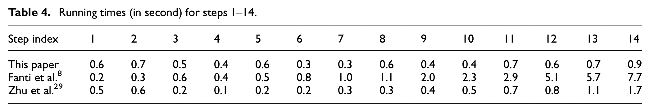
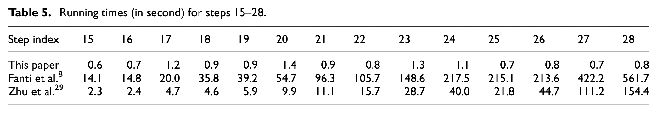
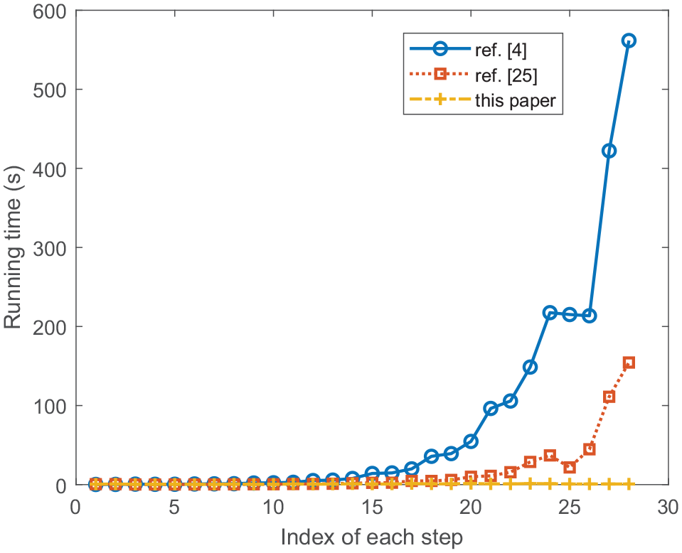
The running times of these three algorithms when observing a step of the corresponding observation are shown in Tables 4 and 5, which are tested on a laptop with Intel Core i7-1165G7 processor and 16G RAM using Gurobi Solver (academic license). ⁴⁶ The relationship of running times of these three approaches in each step is visualized in Figure 12.

Table 4.

Running times (in second) for steps 1–14.

Step index	1	2	3	4	5	6	7	8	9	10	11	12	13	14
This paper	0.6	0.7	0.5	0.4	0.6	0.3	0.3	0.6	0.4	0.4	0.7	0.6	0.7	0.9
Fanti et al. 8	0.2	0.3	0.6	0.4	0.5	0.8	1.0	1.1	2.0	2.3	2.9	5.1	5.7	7.7
Zhu et al. 29	0.5	0.6	0.2	0.1	0.2	0.2	0.3	0.3	0.4	0.5	0.7	0.8	1.1	1.7

Table 5.

Running times (in second) for steps 15–28.

Step index	15	16	17	18	19	20	21	22	23	24	25	26	27	28
This paper	0.6	0.7	1.2	0.9	0.9	1.4	0.9	0.8	1.3	1.1	0.7	0.8	0.7	0.8
Fanti et al. 8	14.1	14.8	20.0	35.8	39.2	54.7	96.3	105.7	148.6	217.5	215.1	213.6	422.2	561.7
Zhu et al. 29	2.3	2.4	4.7	4.6	5.9	9.9	11.1	15.7	28.7	40.0	21.8	44.7	111.2	154.4

Figure 12.

Comparison of approaches in this paper Fanti et al. ⁸ and Zhu et al. ²⁹

We observe that the running times of the approaches in Fanti et al. ⁸ and Zhu et al. ²⁹ significantly increase as the increase of the length of the observation. The main reason for such a situation is that the size of the ILP problems built in Fanti et al. ⁸ and Zhu et al. ²⁹  is linear with the length of an observation. However, the size of the ILP problem constructed in this paper is regardless of the length of an observation, as indicated by equations (6) and (7). Thus, the running time of our approach in each step remains basically the same and does not quickly increase when the observation becomes longer. In this case study, our approach is more efficient in contrast to the ones in Fanti et al. ⁸ and Zhu et al. ²⁹

Conclusion

In this paper, we solve the fault diagnosis problem using Petri net models. Two fault diagnosis algorithms for Petri nets and LPNs are developed, respectively. The proposed approach enjoys higher computational efficiency compared with those in Fanti et al. ⁸ and Zhu et al. ²⁹ and is more suitable for use in real-world systems with low computing power. Future works are two-fold. Firstly, we plan to employ the proposed approach to a real-world system and report its effectiveness. Secondly, the proposed approach will be extended to stochastic Petri nets by associating a firing probability with each transition.