
Abstract
In this paper, we formulate high-type intelligent control as a multi-objective problem and apply evolutionary algorithms to search for optimal solutions. Specifically, we consider the metrics of the system in both the frequency domain and the time domain. Integrated time and absolute error is used as a performance metric in the time domain, while bandwidth is used as a measure in the frequency domain. Simultaneously, the amplitude margin and phase margin are used as constraints to ensure the stability of the high-type control system. Then, we adopt evolutionary algorithms to solve the formulated multi-objective problem. Unlike most of the existing approaches, we formulate intelligent high type control as a multi-objective optimization problem based on our knowledge about the control system. Furthermore, evolutionary algorithms are adopted to search for optimal solutions to real-world controlling systems. Extensive experiments are conducted to evaluate the effectiveness of our proposed approach. Compared to the Z-N method and the extending symmetrical optimum criterion, our proposed method achieves an improvement in bandwidth of more than 126.6%, while reducing the overshoot by more than 56.8% and the settling time by more than 48.4% for all controlled objects used in the experiments. At the same time, the tracking errors of the ramp and parabolic signals are significantly reduced, which means this method effectively improves the system performance.
Introduction
The development in the field of artificial intelligence has led to the advancement of intelligent control. Recently, intelligent control has become a subfield of increasing interest to researchers in industrial control. Intelligent control is a control method with intelligent information processing, intelligent information feedback, and intelligent control decision-making, which mainly solves the control problems of complex systems that are difficult to be solved by traditional approaches. Intelligent control has been studied and applied in industrial fields such as iterative learning control, 1 adaptive cruise control, 2 intelligent microgrids, 3 and controller parameter tuning. 4 The control object of intelligent control is characterized by uncertainty and complexity.
In the study of parameter tuning, controllers’ parameters of high-type control systems often use intelligent optimization methods to solve the problem due to its complexity. The high type controller has a significant advantage in eliminating high type errors such as ramp errors, parabolic errors and can track high order signals quickly. 5 However, the high-type control involves more turning parameters, and the order of the parameters increases, making the system less stable and its optimization more challenging.
In the past decade, tuning laws for high type control have been extensively studied. 6 For instance, Kaya 7 proposed a parameter tuning method based on two degrees of freedom IMC. Tavakoli and Seifi 8 proposed an adaptive self-tuning PID based Lyapunov theory to guarantee the stability of the closed-loop system. Tang et al. 9 proposed a gain-maximizing PI-PI control law to improve the bandwidth and disturbance suppression of the optoelectronic control platform. Papadopoulos et al. 10 designed the control loop of a type-III system by applying the symmetrical optimum criterion to optimize the type-III system based on the proportional-integral-derivative (PID) controller. A loop design for type-p PID control based on the symmetrical optimum criterion is presented in Papadopoulos and Margaris. 11 The type-p system is defined as a control system in which the number of integration controllers is equal to p. 11 It uses a posteriori method to verify the control system’s stability, and additional filters need to be added to achieve improvements in system performance. Hamza et al. 12 used a particle swarm algorithm on the type-II controller in a closed-loop system with a high gain buck-boost converter to improve its efficiency and dynamic response. However, it only optimizes a single time-domain metric like the integrated time and absolute error (ITAE). Since numerical optimization methods, such as mathematical planning and polar value methods, have the disadvantage of high complexity in the parameter rectification problem of high-type control. Traditional single-objective optimization algorithms cannot comprehensively consider the system’s overall control performance.
In high-type intelligent control, both the time domain parameters and the frequency domain parameters are essential to measuring the system’s control performance. Formulas can calculate the relationship between them in systems of type-II and below, but in systems of type-III and above, their relationship may be too complex to be calculated explicitly. 13 Most of the existing controller design methods consider both time domain and frequency domain metrics linearly by combining a series of multiple metrics into a single scalar target. 14 In practice, however, it is difficult to determine the weights of individual indicators because the effect of optimal control is usually unknown. Simultaneously, the increase in system type means an increase in controller parameters, which poses difficulties for traditional numerical optimization algorithms; high type control also faces the problem of instability due to the high number of system types.
In this work, we formulate high-type intelligent control as a multi-objective problem and apply evolutionary algorithms to search for optimal solutions. Specifically, we consider the metrics of the system in both the frequency domain and the time domain. Simultaneously, the amplitude margin and phase margin are used as constraints to ensure the stability of the high type control system. Then, the state-of-the-art evolutionary algorithms are exploited to solve the formulated multi-objective problem.
In contrast to the high-type controller obtained by the symmetrical optimum criterion: the controller in this paper does not need to add additional filters based on the designer’s experience to obtain better control effects in practice; in contrast to the method using zero-pole elimination: the model mismatch caused by the identification error will cause a significant reduction in the control performance of the system, while the method in this paper does not rely on zero-pole elimination and has a significant improvement in disturbance rejection ability. In summary, the controllers optimized by multi-objective optimization are effective in reducing the steady state error, overshoot, settling time and improving disturbance rejection ability of the system, which are also demonstrated in the subsequent experimental results.
The novelty and contributions of this work can be summarized as follows:
We formulate the high-type intelligent control as a multi-objective optimization problem by combining the bandwidth and ITAE indicators in both the time domain and frequency domain. The proposed approach provides the users a set of trade-off solutions on desired objectives, which is greatly useful in many real-world applications.
An apriori stability constraint is adopted to ensure the stability of the system. It involves knowledge about the control system in our problem formulation. As a result, the optimized control system can directly meet the engineering requirements.
We apply evolutionary optimization algorithms to solve the formulated multi-objective problems about different types of control systems. We select suitable optimization algorithms for controller parameter tuning for different problems and discuss the advantages and disadvantages of the evolutionary algorithms in solving system control problems under different settings. The provided selection strategy may be helpful for the algorithm designers in this field.
The rest of this article is as follows. Section 2 introduces the high-type control. Some basic concepts, definitions, and existing control systems are illustrated. The optimization objectives and stability constraints of the control system are presented in Section 3. Next, the multi-objective evolutionary algorithms are introduced in Section 4. Finally, we report the simulation results and comparisons for different types of controlled objectives using different optimization algorithms in Section 5.
High-type control
Definitions and preliminaries
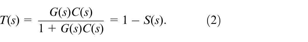
A typical feedback control system, as shown in Figure 1, is a system in which the output signal is sampled and then feed back to the input to form an error signal that drives the system. We define a sensitivity function
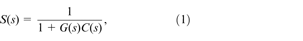
where
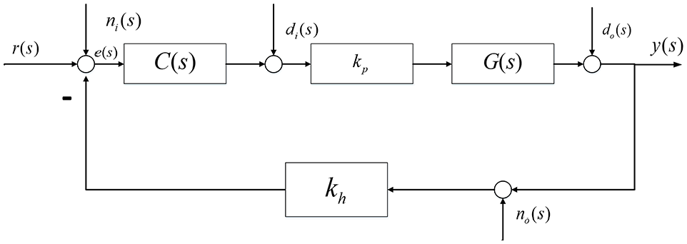
Block diagram of a classic control system,
11
where
It is a transfer function from the reference signal
PID control
In industrial applications, the controlled object
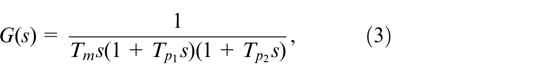
where
In Figure 1, the controller
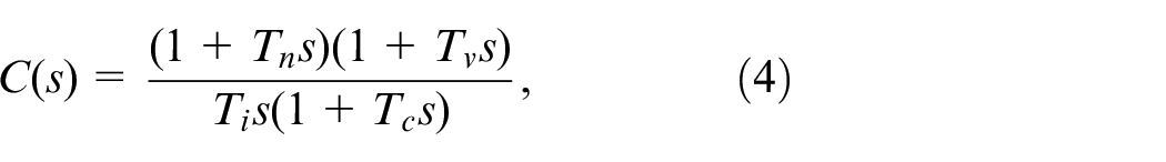
where
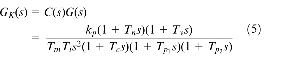
Thus, the open-loop transfer function of the system
and the closed loop transfer function of the system
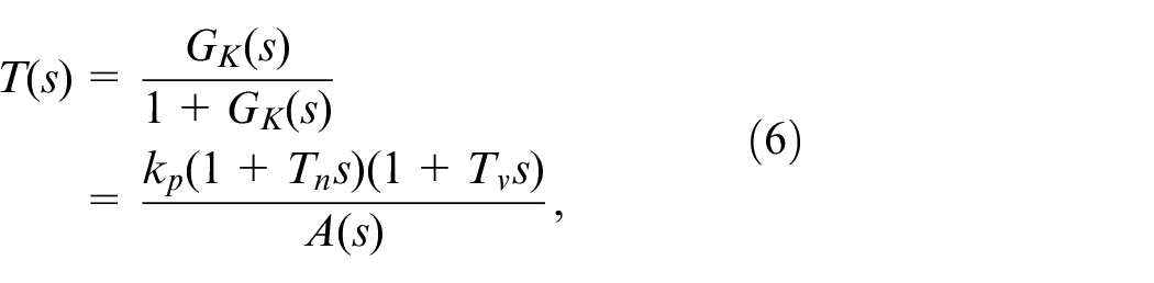
where,
The error transfer function of the system
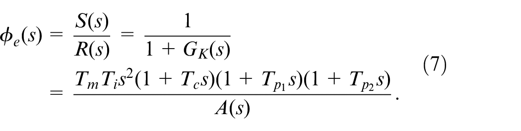
According to the final value theorem from Dorf and Sinha, 16 the steady-state error of the system can be expressed as:
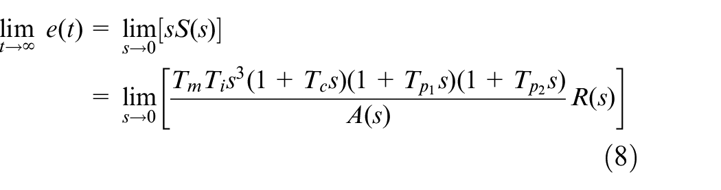
When the reference input signal is a step signal, that is to say

When the reference input signal is a ramp signal, which indicates
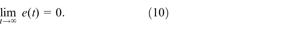
When the reference input signal is a ramp signal, which means
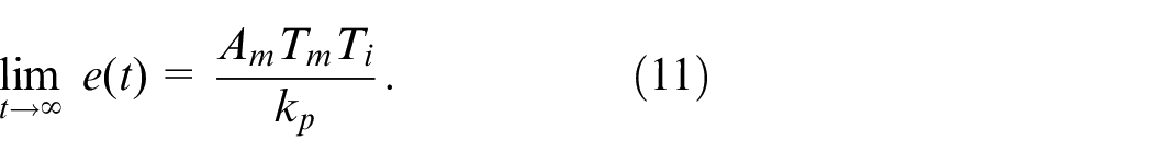
From equation (9), it can be seen that the steady-state error is zero when the PID controller tracks the step signal and ramp signal. 17 However, from equation (11), the steady-state error is a constant value when the PID controller tracks the parabolic signal. In many practical industrial applications, the control system is usually designed to be at least a type-I control system. 11
Type-III system with I-PID controller
Based on the above analysis, PID controllers are limited to eliminate higher-order tracking errors, which can be effectively addressed by forming higher-order controllers through series integrators. 18 When the system uses a high-type controller I-PID with a series integrator, the controller can be defined as:
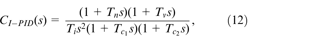
where
The open-loop transfer function of the system is:
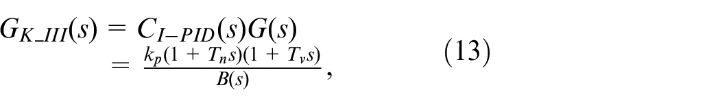
where,
And the closed loop transfer function of the system is
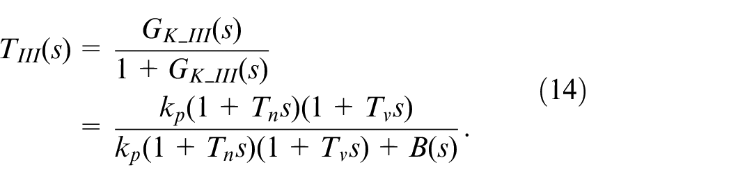
We have the error transfer function of the system as
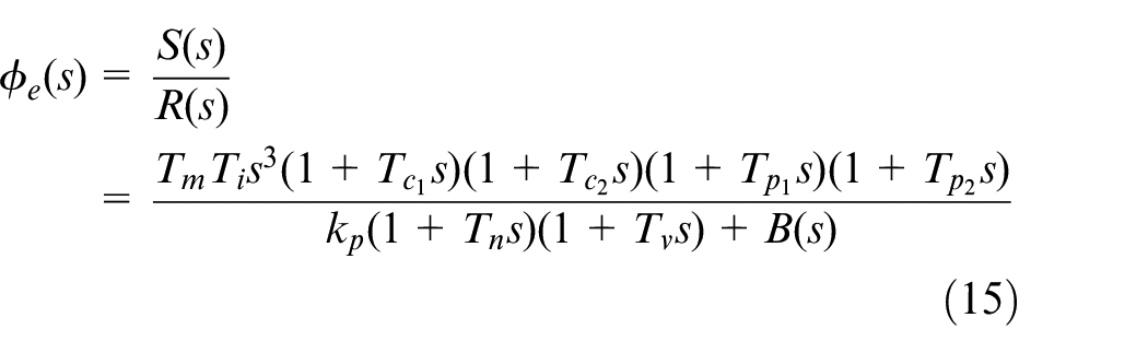
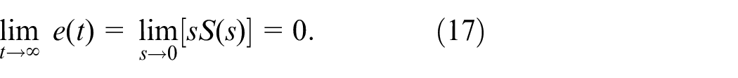
Similarly, based on the final value theorem, the steady-state error of the system can be expressed as:
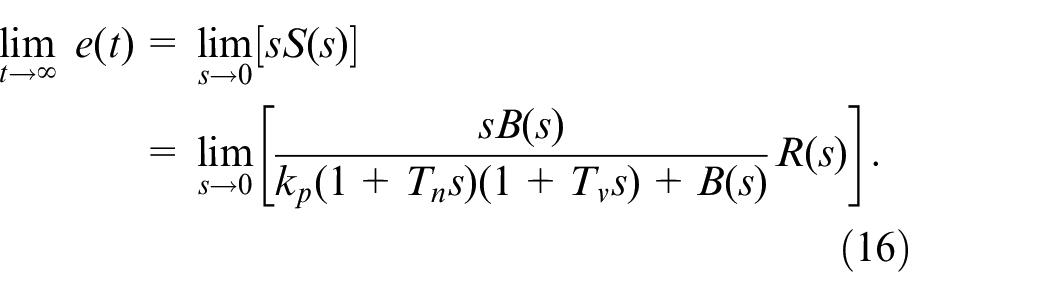
When the reference input signal is a step signal, that is to say
When the reference input signal is a ramp signal, which means

When the reference input signal is a parabolic signal, which indicates
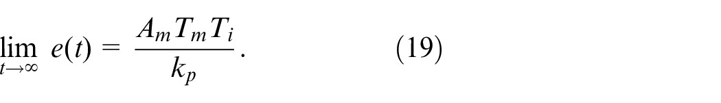
From equations (17), (18), and (19), it can be seen that the type-III system with the addition of the proportional controller achieves zero error in tracking the step signal, ramp signal, and parabolic signal. It also shows the superiority of the type-III system in tracking higher order errors.
Evidenced by the same token, there is a significant advantage in tracking higher-order errors when the type of system are greater than type-III.
Extension of type-p system
Based on the analysis in sections 2.2 and 2.3, the controller is extended to a type-p system, 11 where p represents the number of proportional controllers in the system’s open-loop transfer function.
We define the object
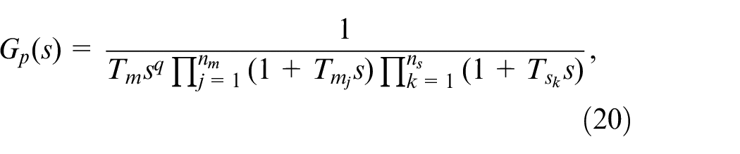
where
where
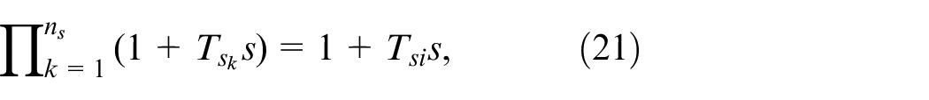
To guarantee the transfer function of a controller to be strictly causal, the order of the denominator must be greater than or equal to
where
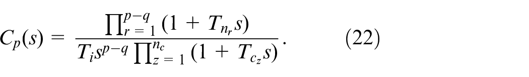
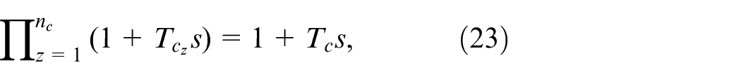
Thus, the open-loop transfer function of the system is
where
And the closed-loop transfer function of the system is

From the analysis of the type-III control system for I-PID in Section 2.3, it can be inferred that the higher type system than the type-III system has a significant advantage in the suppression of higher-order errors.
Multi-objective optimization for type-p system controllers
Multi-objective problem formulation
Objective functions
In intelligent control systems, frequency domain parameters and time domain parameters are critical indicators for measuring system control performance. The frequency-domain indicators are more concise and profound, while the time domain indicators are more intuitive. In the low-order system, we can calculate according to the formula to get the relationship between the frequency domain indicators and time-domain indicators. 19 However, when the system type is higher than the second order, the constraint relationship between them can not be obtained through a simple calculation method. Therefore, we use a combination of frequency domain and time domain indicators to integer the controller’s parameters.
Bandwidth indicator in frequency domain
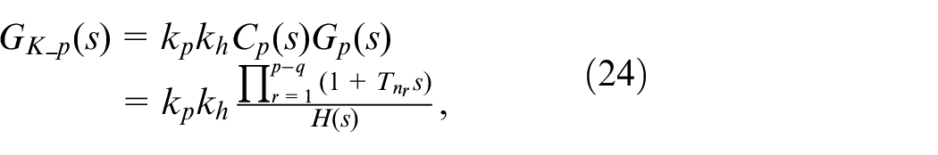
The bandwidth of a closed-loop system is an important measure of the system’s ability to track signals. 20 The wider the bandwidth means the wider the tracking band available to the system. Both the symmetrical optimum criterion 11 and amplitude optimal methods use maximum bandwidth as the optimization goal. For the type-p system mentioned in Section 2.4, the open-loop transfer function is defined as:
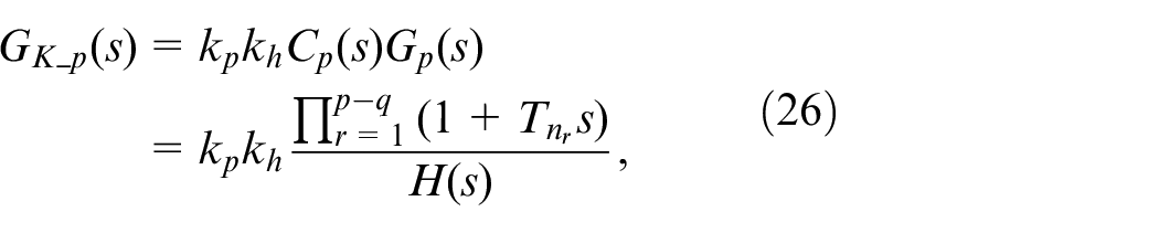
and the closed-loop transfer function is defined as:
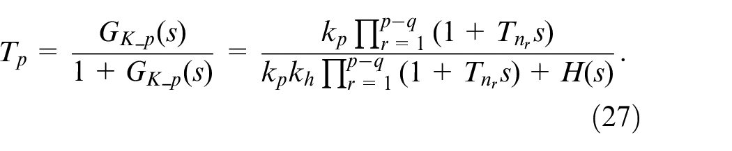
To maximize the closed-loop bandwidth of the system,
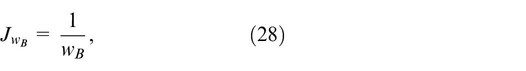
where w is calculated as

and
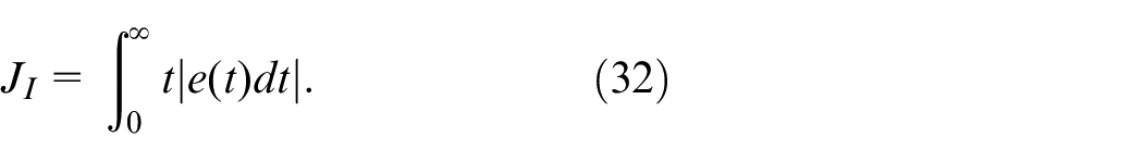
Performance indicator ITAE in time domain
The frequency-domain objective of bandwidth is insufficient to reflect the system’s response to transient signals, so a comprehensive metric in the time domain is used to measure the system’s step-response performance. When performing controller parameter tuning, a suitable objective function is proposed for different production processes and different control purposes. There are two commonly used metrics. One is a single performance metric based on the system’s closed-loop response characteristics, such as steady-state error, regulation time, and oscillation period. This individual performance indicator is intuitively simple and meaningful, but it is less accurate and biased in the calculation process. The other is a performance indicator that contains the integral of a function of the control system’s steady-state error, which can reflect the overall performance of the system’s dynamic response. 21 Most studies consider the integral of the time weighted absolute error value (ITAE) as one of the best indicators of performance for single-input single-output control systems. 22 The control system designed according to the ITAE principle has a small oscillation of transient response, which is a good engineering practicality and selective control system performance evaluation index.
The calculation of ITAE is as follows:
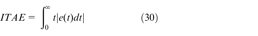
where
In discrete systems, the discrete ITAE indicator takes the form of:
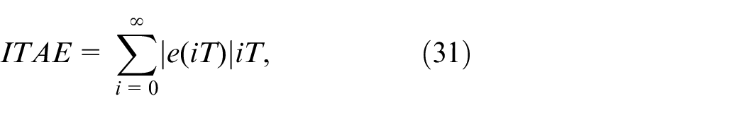
where
The ITAE indicator of the type-p system’s optimization is expressed as:
Constraints
For a control system, stability is a necessary condition to ensure the proper operation of the system. 23 There are many methods to ensure stability, such as the Lyapunov criterion 24 and the Routh criterion in the time domain, the Nyquist criterion and the margin criterion in the frequency domain, and so on. In this work, we use the stability margin criterion in classical control, including phase margin and amplitude margin. In engineering applications, a system that satisfies the amplitude margin is more than 6 dB and the phase margin is more than 45º is considered to be stable. For a system constituting a type-p system, to ensure the system be stable we present the constraint on the amplitude margin that

where

and the constraint on the phase margin is defined as
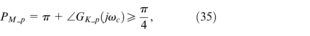
where

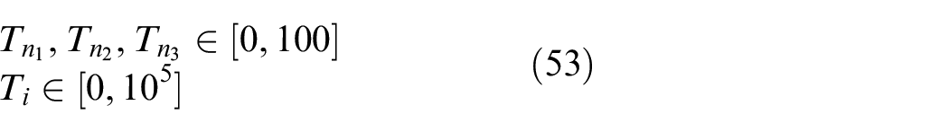
The ranges of variables
The selection of the optimization parameter scope also has an important impact on the algorithm’s search results. In this work, the parameter ranges are fully conditioned using the Routh criterion. 25 The range of controller parameters is discussed as an example of parameter range selection for a type-III system.
The characteristic polynomial for a type-III system is:
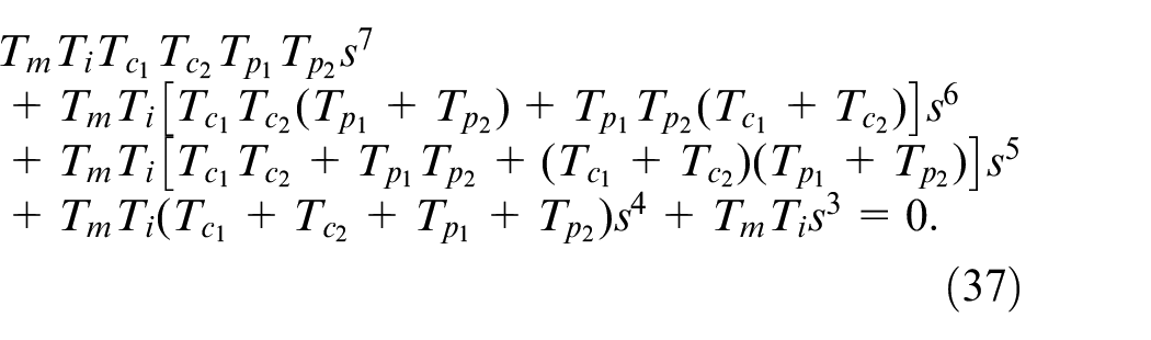
It leads to the following results:
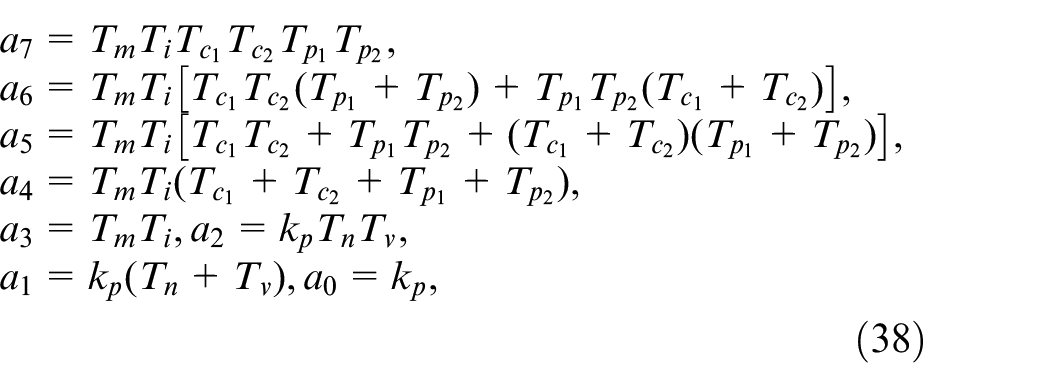
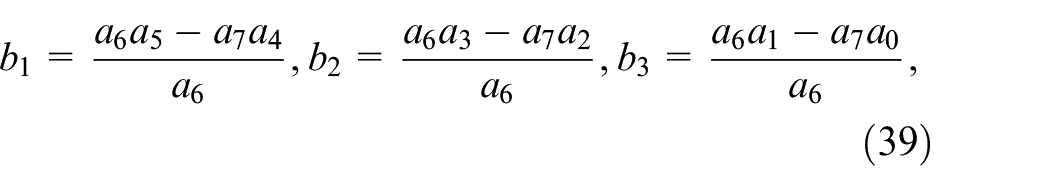
Based on
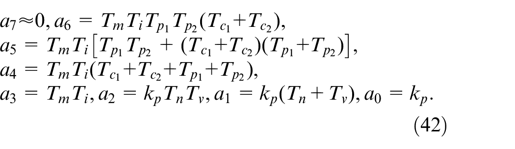
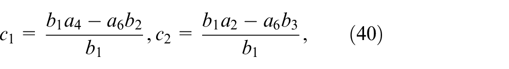
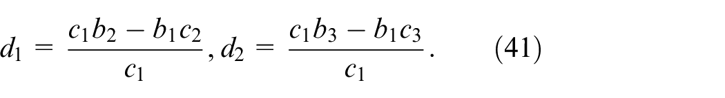
From equation (42), we have the results of equations (39), (40), and (41) as
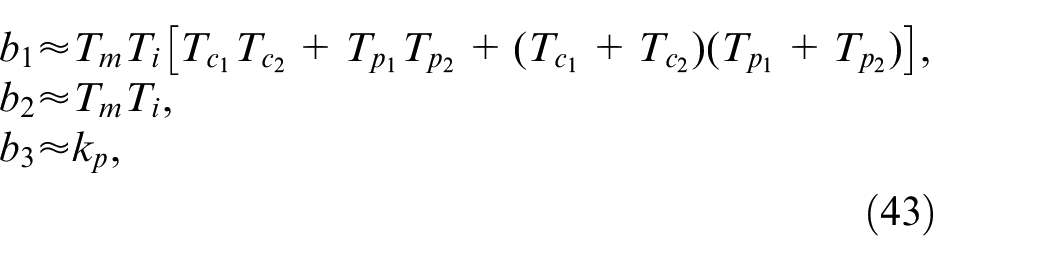
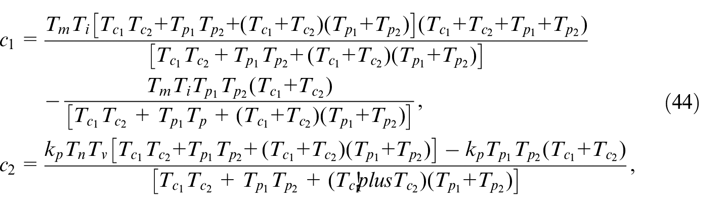
and
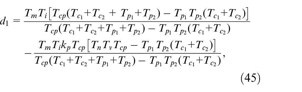
where
According to the Routh criterion,
25
the parameter should satisfy the condition
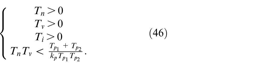
The parameter selection range for the type-p system can also be obtained by referring to the solution method for the type-III system.
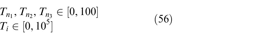
Based on the objective functions and constraints presented in the above sections, the multi-objective problem of type-p control is formulated as:
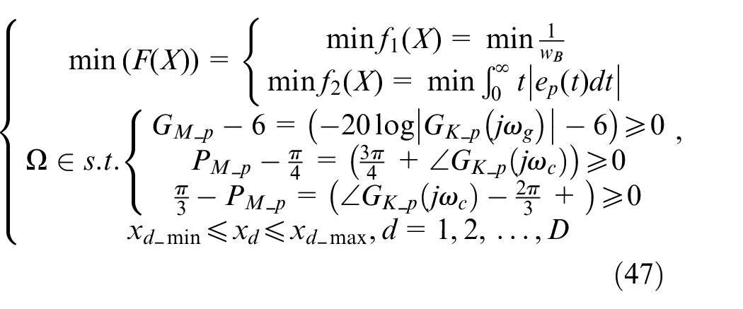
where the decision variables in
Multi-objective optimization using evolutionary algorithms
In general, multi-objective optimization algorithms can be divided into two categories: traditional optimization algorithms and intelligent optimization methods. Traditional methods include mathematics programming, weighting methods, etc., but usually only one of the Pareto solutions can be obtained at a time. However, intelligent optimization methods will get more Pareto solutions or even complete Pareto solutions. Therefore, we selected different types of evolutionary algorithms(EAs) for solving the formulated problem.
In this section, we utilize evolutionary algorithms to solve the formulated multi-objective problems. 26 Since the problem is often composed of multiple conflicting objectives, the solution to the problem is usually not a single optimal solution, but a set of Pareto solutions.27,28 Evolutionary algorithms simulate the evolutionary mechanism of organisms and solve the multi-objective optimization problems in a parallel manner. Depending on different selection mechanisms, EAs can be broadly classified into three categories: decomposition-based algorithms, indicator-based algorithms, and Pareto dominance-based algorithms.
Decomposition-based algorithms typically decompose a complex multi-objective problem into multiple sub-problems. By solving the sub-problems collaboratively, the solution set of the original complex problem is obtained. The Multi-objective Genetic Local Search (MOGLS) algorithm 29 uses combinations of objective functions with different weights as the adaptation function values, and in each iteration, generates a random weight is used to aggregate the objectives of the problem. The Multi-objective Evolutionary Algorithm Based on Decomposition (MOEA/D) proposed by Zhang et al. 30 transformed a multi-objective optimization problem into a number of columns of single-objective problems and evolves the population in a synergistic manner.
Indicator-based algorithms use a performance metric to guide the choice of search and settlement during the evolution of the algorithm. Indicator-based evolutionary algorithm (IBEA) 31 is pioneering work in this class of algorithms. IBEA uses one metric to evaluate and compare the performance of a pair of candidate solutions, eliminating the need for similar distributional retention mechanisms such as adaptation efficacy. Metrics based on hypervolume can effectively improve the convergence and diversity of populations. 32 However, high computational complexity and long computation time are disadvantages of such algorithms.
Pareto domination-based algorithms are the most widely used multi-objective optimization algorithms. The basic idea of this type of methods is to select the optimal solution based on the dominance relationship between the solutions and the density of the solution. The first layer selection is based on the dominance relationship between the solutions, so that the solution set converges gradually. Then the second level selection is made based on the density of solutions to optimize the diversity of the population. Representative methods include NSGA-II, 33 NSGA-III, 34 SPEA2, 35 etc.
NSGA II is a popular multi-objective evolutionary algorithm for two or three objectives. It is used in the paper Ayala and Coelho 36 and Sutha and Thyagarajan 37 as a tool for parameter tuning of the controllers. NSGA III is an improvement algorithm of NSGA II, which introduces the setting of reference points in contrast to NSGA II. In the paper Shen, 38 it is applied to the problem of fractional order controller tuning. The SPEA 2, a modification of the SPEA, is applied to the tuning of a PID controller for a boiler superheated steam temperature cascade control system in Xia. 39 In Gacto et al., 40 the authors use SPEA 2 to optimize fuzzy controllers in ventilation and air conditioning systems. Both RVEA and NSGA III are evolutionary algorithms based on reference points, but the reference vectors of the RVEA are adaptively adjusted, and it is an algorithm for many-objective problems.
Since in multi-objective optimization, there is generally no solution that optimizes all objectives. The concept of the Pareto solution is defined. The solutions in a Pareto solution set satisfy a certain Pareto domination relation, where each solution is contained in the Pareto Front. 41 From the application of multi-objective optimization algorithms for controller parameter rectification, it can be seen that multi-objective based controller parameter tuning is a promising research direction.
However, most of the existing studies adopt a multi-objective optimization method for the type-I or type-II system for parameter tuning. In this work, various multi-objective optimization algorithms are used to optimize and tune the parameters of type-III systems for different controlled objects. We aim to select the most suitable one for the target intelligent controller and provide some guidelines for the researchers and practitioners in multi-objective intelligent control.
Simulation results
To verify the effectiveness of evolutionary optimization algorithms in parameter optimization of the type-p controller, we use the controlled objects in Papadopoulos and Margaris. 11 Control simulation examples of type-III systems for different objects are provided. The effects of type-I and type-III systems on the control of the same controlled object are also compared. Multi-objective optimization algorithms, including NSGA-II, NSGA-III, SPEA2, RVEA, MOEA/D, and IBEA, are applied to optimize different controlled objects.
Process with dominant time constants (object 1)
For a controlled object with dominant time constants, the transfer function can be described as:
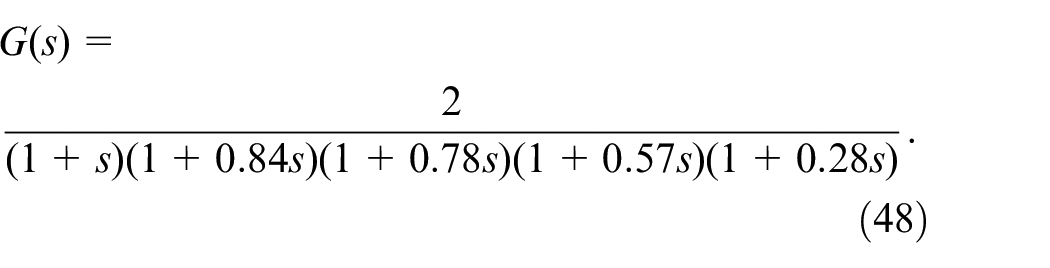
The I-I-PID controller, defined in equation (49), is used to form a type-III system with the object in equation (48):
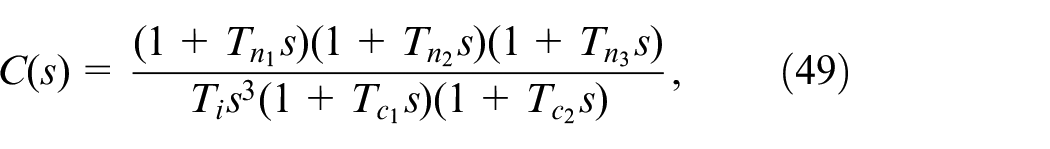
where
Optimization parameter solution set is

The initial population number is 100, and 10,000 iterations are performed. Each algorithm is repeated five times to eliminate the effect of algorithm randomness on the optimization results. To evaluate the performance of different evolutionary algorithms, We need to calculate some commonly used indicators in the field of multi-objective optimization, such as inverted generational distance (IGD), hypervolume (HV), etc. 42 In Li et al., 43 it is stated that IGD is a distance-based quality indicator and HV is a volume-based quality indicator. Both IGD and HV measure the all quality aspects performance of the resulting solution set. Also, as mentioned in Li and Yao, 44 the IGD indicator prefers uniformly distributed solutions, while the HV indicator prefers knee solutions. For the controller parametric tuning problems, the set of reference points and the true pareto surface of the optimal solution are not known in advance, therefore, it is not appropriate to use the IGD indicator. In the case of parameter tuning problems, we are actually more interested in the existence of solutions that achieve better control, so in this paper we have chosen the HV indicator as a criterion for judging the optimization results of several algorithms.
The HV calculates the hypervolume of the objective space between given solution sets and given reference points.
45
The reference points chosen should be those that are worse than the estimated pareto solution set.
32
Based on the optimization results of the problem, we set the reference point as
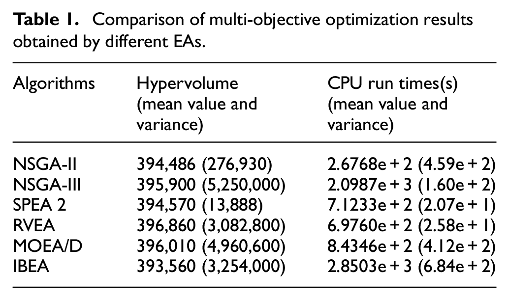
The hypervolume values and CPU run times of the recorded optimized solution sets are reported in Table 1, from which we have the following observations:
(1) The HV value of the solution sets obtained by the six algorithms are less different. The RVEA has the largest HV value, and the IBEA has the smallest HV value.
(2) The SPEA2 has the smallest HV variance, and the NSGA-III has the largest HV variance. This indicates that the SPEA2 has better stability relative to NSGA-II in terms of parameter optimization for this object.
(3) In terms of CPU runtime, algorithm NSGA-II consumes the least amount of time, and IBEA consumes significantly more time than the other algorithms.
(4) 2Taken together, IBEA performs relatively poorly in optimizing object 1, while NSGA-II performs relatively well.
Comparison of multi-objective optimization results obtained by different EAs.
Since the HV values obtained by several algorithms are not very different, and the NSGA-II has a significantly shorter optimization time, we choose NSGA-II to optimize the controller’s parameters of the process with dominant time constants. The optimized solution sets obtained by NSGA-II are shown in Figure 2, where the blue points are the solution sets obtained by NSGA-II, and the red points indicate the non-dominated solutions in the obtained solution set.
Results of the run with the largest hypervolume value on object 1 (process with dominant time constants).
By selecting a set of controller parameters with the smallest ITAE value, we show the controller as:
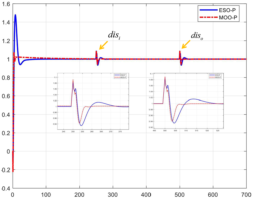
The step response of the type-III closed-loop system is shown in Figure 3. MOO-P is the type-p system that uses multi-objective optimization (MOO), and ESO-P is the type-p system that uses the extended symmetrical optimum criterion (ESO). The ESO-P system has an overshoot of 43.3%, while the MOO-P system has an overshoot of 18.7%. At the same time, adds disturbance
Comparison of step response (object 1).
From Figure 3, when adding step disturbance
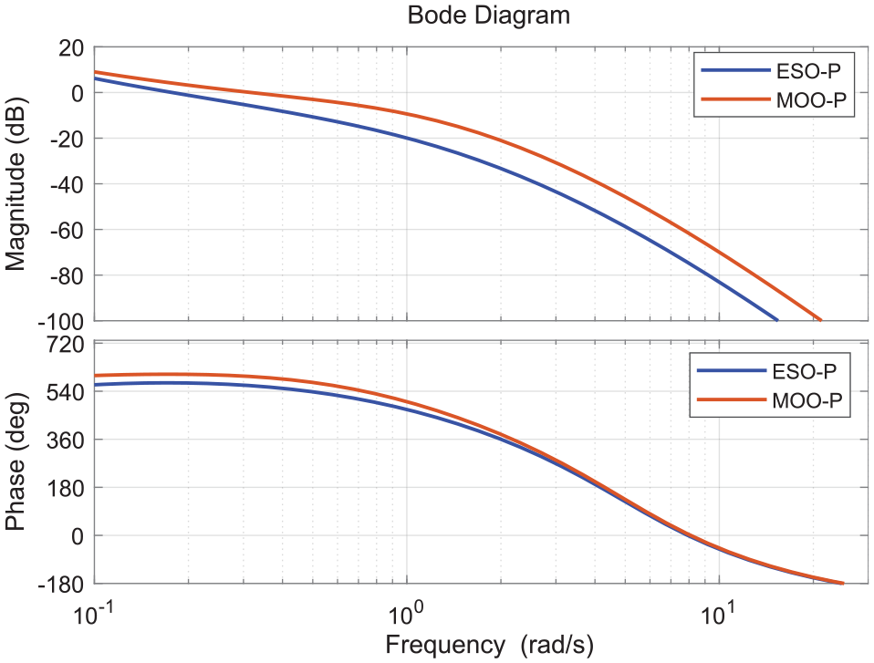
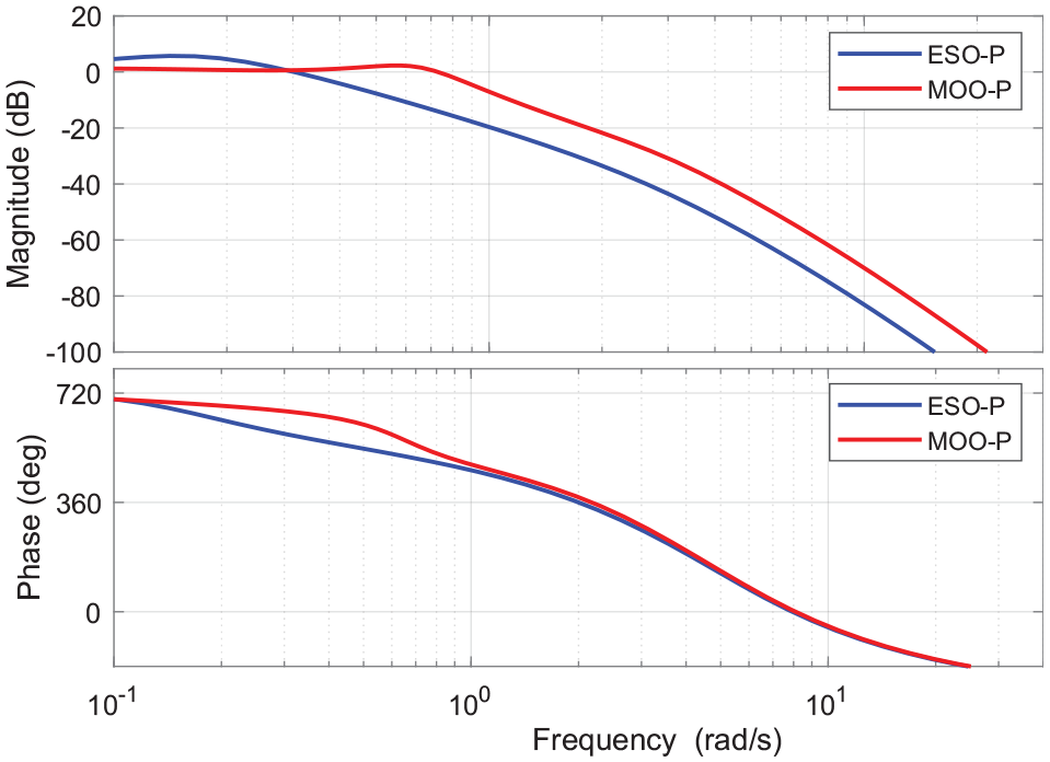
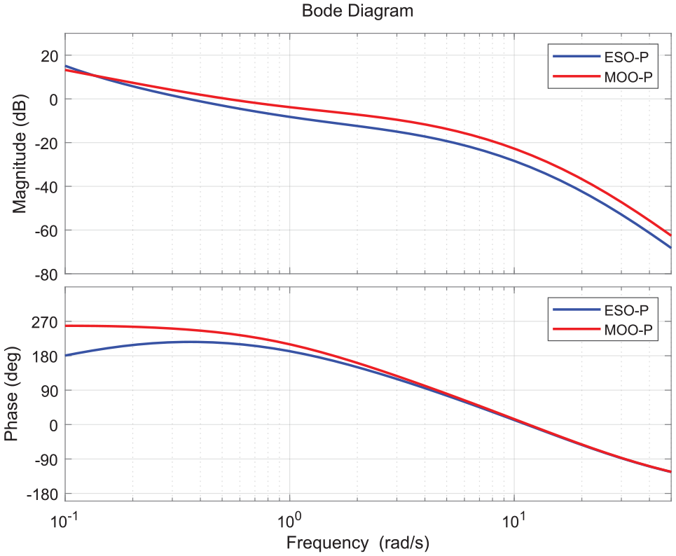
The bode diagram of the open-loop and closed-loop of the control system are shown in Figures 4 and 5. The ESO-P system has a phase margin of 40º and an amplitude margin of 15.28 dB. The MOO-P system has a phase margin of 56.3º and an amplitude margin of 6 dB. Compared to the ESO-P system, the MOO-P system has a larger phase margin, which means MOO-P is more stable.
Comparison of open-loop bode diagrams (object 1).
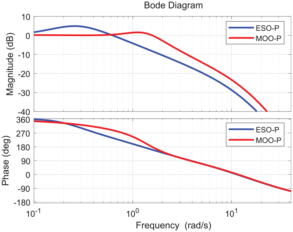
Comparison of closed-loop bode diagrams (object 1).
From Figure 5, the system’s bandwidth of ESO-P is 0.0461 Hz, while that of MOO-P is 0.1743 Hz. Compared with ESO-P, the bandwidth of MOO-P increased 278.9%.
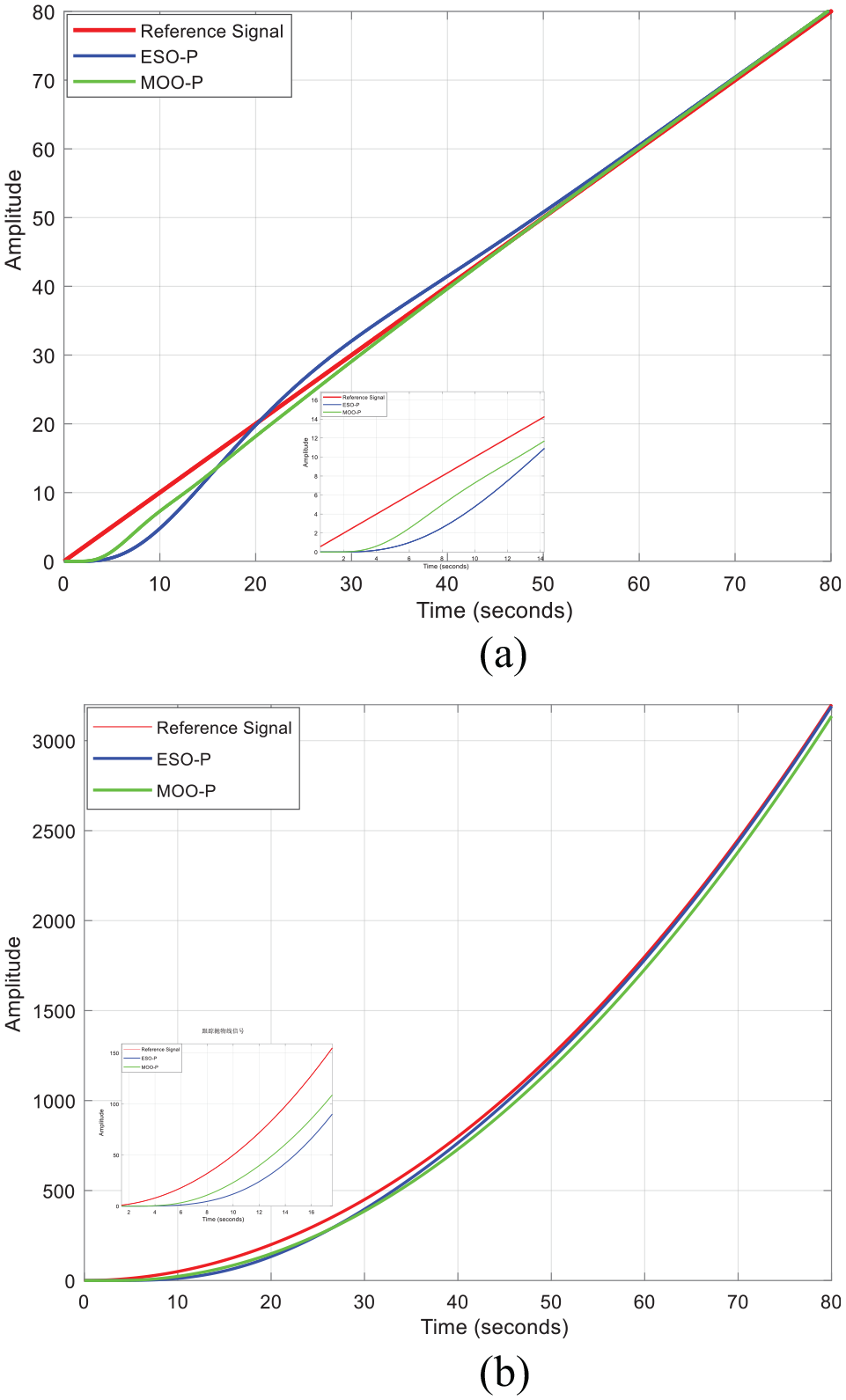
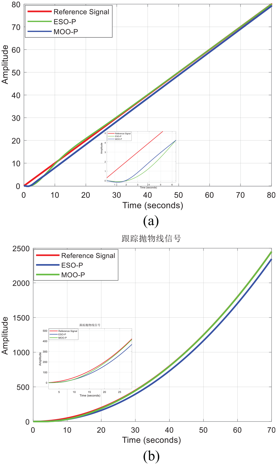
The tracking of the ramp and parabolic signals by the closed loop system is shown in Figure 6, As can be known from the Figure 6, the MOO-P system has a smaller tracking error than the ESO-P system in tracking ramp signals and parabolic signals, and can achieve faster signal tracking. Therefore, the MOO-P system is more advantageous in tracking higher-order signals.
Comparison of signal tracking (object 1): (a) comparison of ramp signal tracking and (b) comparison of parabolic signal tracking.
Process with time delay (object 2)
For a controlled object with time delay, the transfer function can be described as:
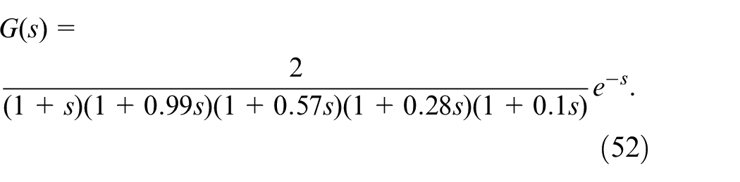
Optimization parameter solution set of the I-I-PID controller is
The initial population number is 100, and 10,000 iterations are performed. Each algorithm is repeated five times to eliminate the effect of algorithm randomness on the optimization results. The HV values and CPU run times of the recorded optimized solution sets are shown in Table 2.
Comparison of HV values obtained by different EAs on process with time delay.
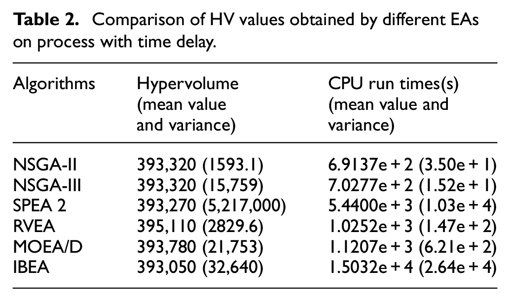
From the results in the table, the following conclusions can be drawn:
(1) The HV values of the solution sets obtained by the six algorithms are less different. The RVEA has largest HV value and the IBEA has smallest HV value.
(2) The NSGA-II has the smallest HV variance and the SPEA 2 has the largest HV variance. This indicates that the NSGA-II has better stability relative to SPEA 2 in terms of parameter optimization for this object.
(3) In terms of CPU runtime, algorithm NSGA-II consumes the least amount of time, and IBEA consume significantly more time than the other algorithms.
(4) Taken together, IBEA performs relatively poorly in the optimization of object 2, while NSGA-II performs relatively well.
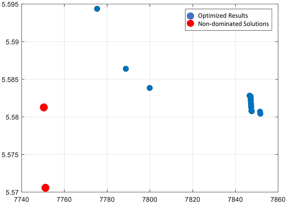
The variance of HV obtained by several algorithms is not much, but the NSGA-II algorithm has the least variance of HV and also has the least running time. Therefore, we choose the NSGA-II algorithm for optimization of the process with time delay. Considering the optimization performance and running time of the algorithms, we select the optimization result of NSGA-II on object 2 as the controller parameter. The optimized solution set obtained by NSGA-II is shown in Figure 7, where the blue points are the solution sets obtained by the NSGA-II, and the red points indicate the non-dominated solutions in the obtained solution set.
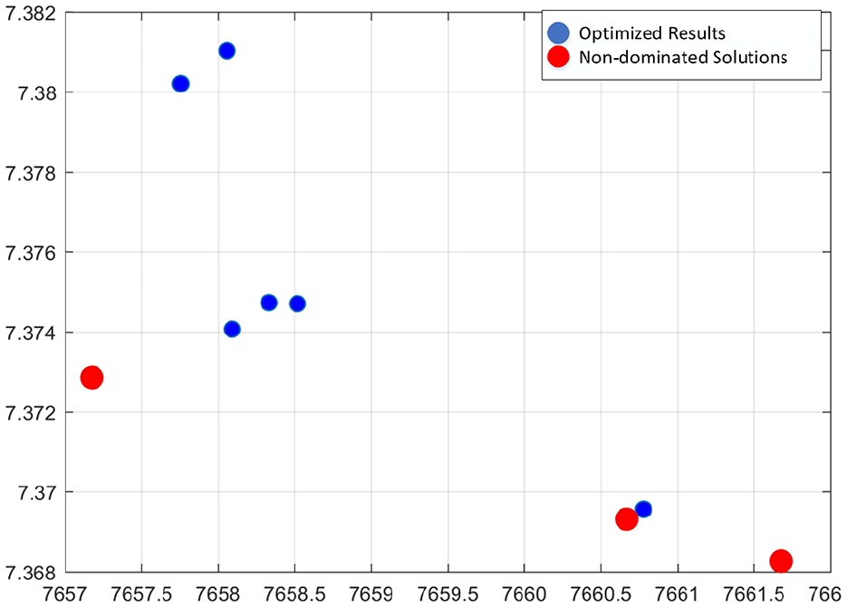
Results of the run with the largest hypervolume value on object 2 (process with time delay).
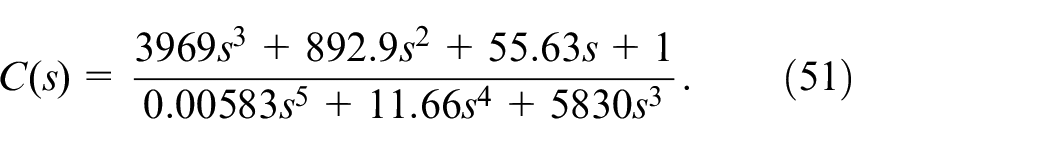
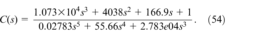
Select a set of controller parameters with the smallest ITAE value and the controller is shown as:
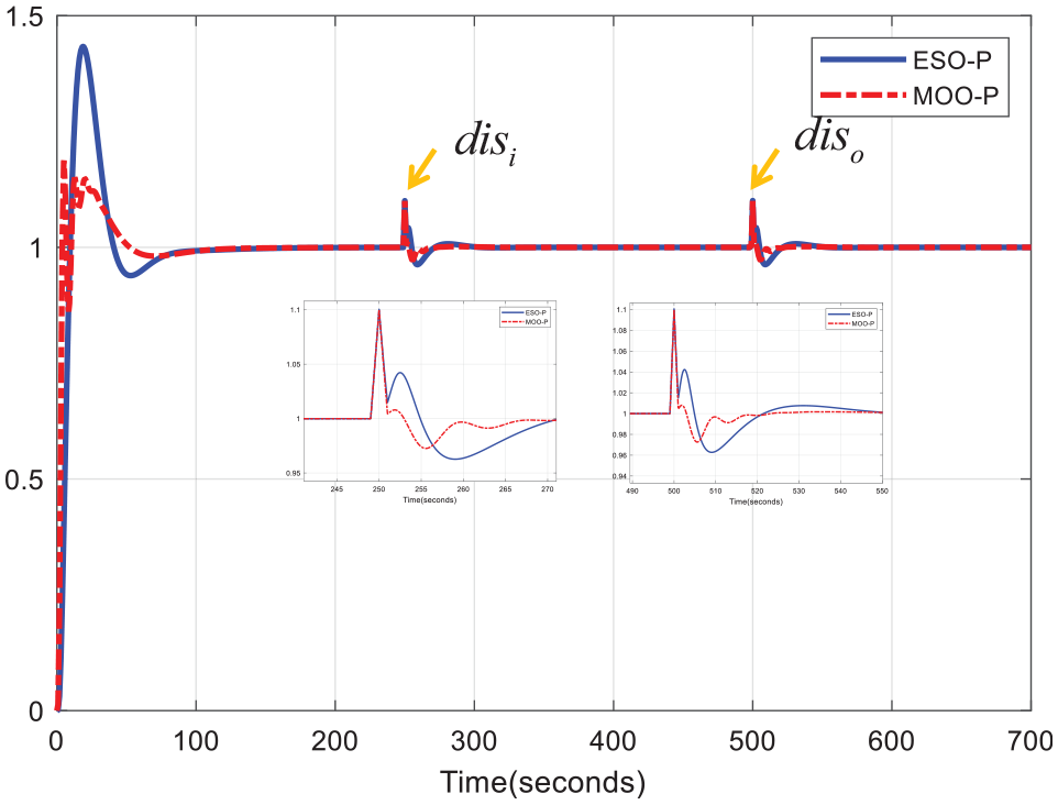
The step response of the type-III closed-loop system is shown in Figure 8. The control system optimized using the symmetry principle has an overshoot of 55.7%, while the control system using this method has an overshoot of 22.7%.
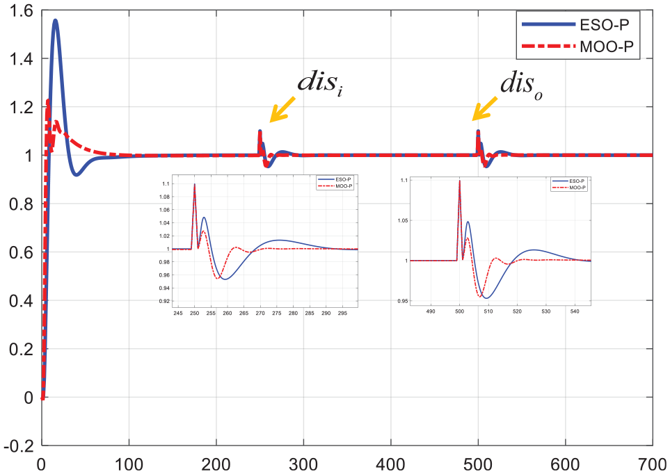
Comparison of step response (object 2).
At the same time, adds disturbance
From the Figure 8, when adding step disturbance
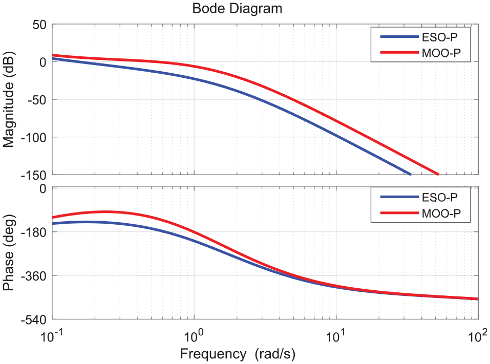
The bode diagrams of the open-loop and closed-loop of the control system are shown in Figures 9 and 10.
Comparison of open-loop bode diagrams (object 2).
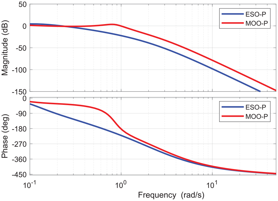
Comparison of closed-loop bode diagrams (object 2).
The ESO-P system has a phase margin of 31.4275º and an amplitude margin of 10.3104 dB. The MOO-P system has a phase margin of 55.1915º and an amplitude margin of 5.9936 dB. Compared to the ESO-P system, the MOO-P system has a larger phase margin, which means MOO-P is more stable.
From Figure 10, the system’s bandwidth of ESO-P is 0.0591 Hz, while that of MOO-P is 0.1339 Hz. Compared with ESO-P, the bandwidth of MOO-P increased 126.6%.
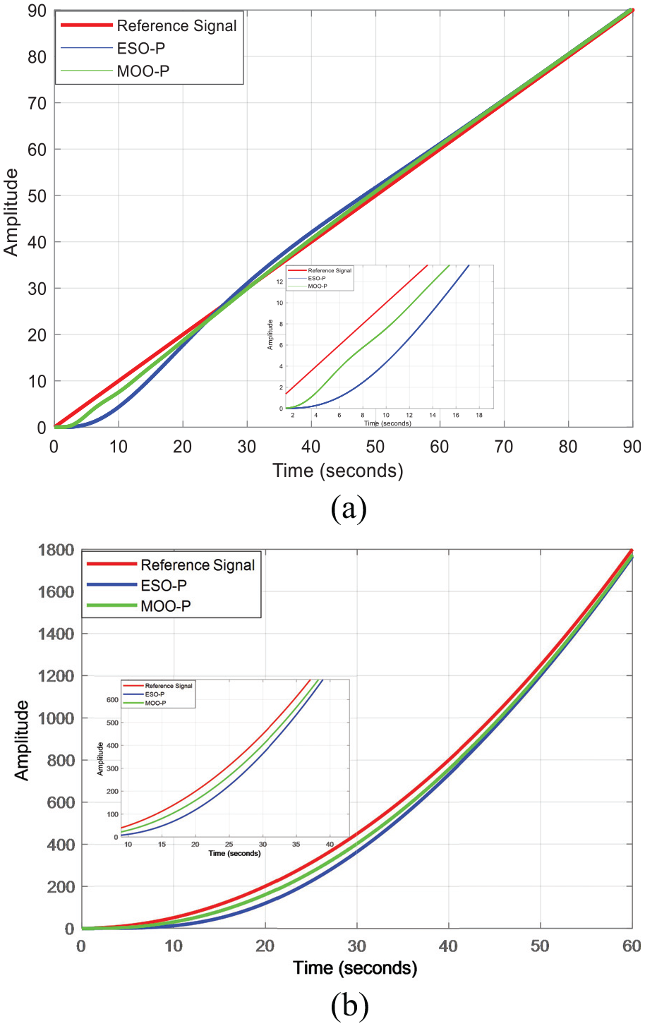
The tracking of the slope and parabolic signals is shown in Figure 11, As can be known from the Figure 11, the MOO-P system has a smaller tracking error than the ESO-P system in tracking ramp signals and parabolic signals, and can achieve faster signal tracking. Therefore, the MOO-P system is more advantageous in tracking higher-order signals.
Comparison of signal tracking (object 2): (a) comparison of ramp signal tracking and (b) comparison of parabolic signal tracking.
Non-minimum phase process (object 3)
For a non-minimum phase process, the transfer function can be described as:
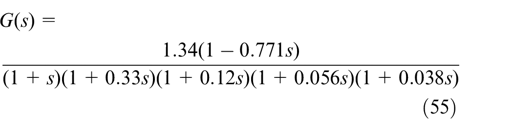
Optimization parameter solution set of the I-I-PID controller is
The initial population number is 100 and 10,000 iterations are performed. Each algorithm is repeated five times to eliminate the effect of algorithm randomness on the optimization results. The HV values and CPU run times of the recorded optimized solution sets are shown in Table 3.
Comparison of multi-objective optimization results.
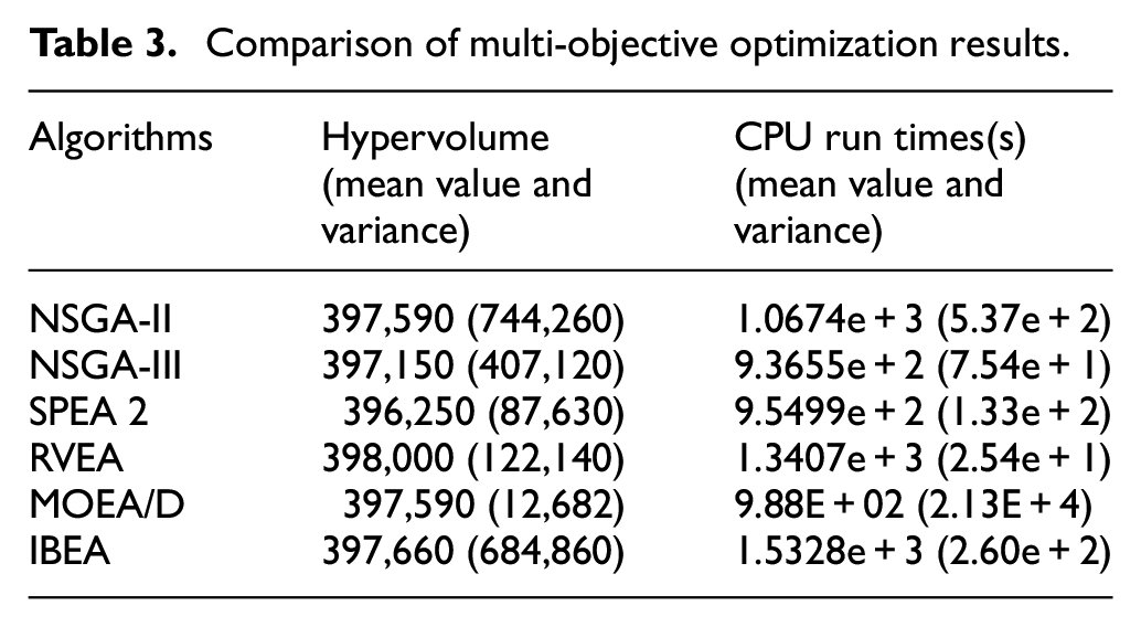
From the results in the table, the following conclusions can be drawn:
(1) The HV values of the solution sets obtained by the six algorithms are less different. The RVEA algorithm has the largest HV value, and the IBEA has the smallest HV value.
(2) The MOEA/D has the smallest HV variance, and the NSGA-II has the largest HV variance. This indicates that the MOEA/D has better stability relative to NSGA-II in terms of parameter optimization for this object.
(3) In terms of CPU runtime, algorithm NSGA-III consumes the least amount of time, and IBEA consumes significantly more time than the other algorithms.
(4) Taken together, IBEA performs relatively poorly in optimizing object 3, while NSGA-III performs relatively well.
The variance of HV obtained by several algorithms is not much, but the NSGA-III algorithm has the least variance of HV and also has the least running time. Therefore, we choose the NSGA-III algorithm for optimization of the non-minimum phase process. The optimized solution set obtained by NSGA-III is shown in Figure 12.
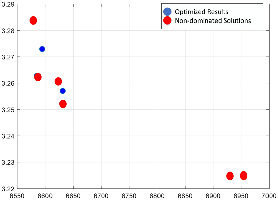
Results of the run with the largest hypervolume value on object 3 (non-minimum phase process).
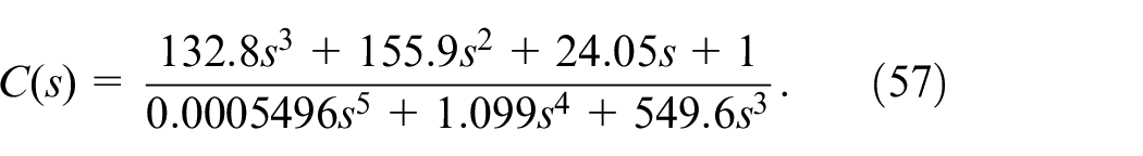
Select a set of controller parameters with the smallest ITAE value and the controller is shown as:
The step response of the system after adopting the type-III closed-loop system is shown in Figure 13. The control system optimized using the symmetry principle has an overshoot of 48%, while the control system using this method has an overshoot of 8%. At the same time, adds disturbance
Comparison of step response (object 3).
From Figure 13, when adding step disturbance
The bode diagrams of the open-loop and closed-loop of the control system are shown in Figures 14 and 15.
Comparison of open-loop bode diagrams (object 3).
Comparison of closed-loop bode diagrams (object 3).
The ESO-P system has a phase margin of 36.1438º and an amplitude margin of 9.6790 dB. The MOO-P system has a phase margin of 58.3806º and an amplitude margin of 5.9967 dB. Compared to the ESO-P system, the MOO-P system has a larger phase margin, which means the MOO-P system is more stable. From Figure 15, the system’s bandwidth of ESO-P is 0.1398 Hz, while that of MOO-P is 0.3233 Hz. Compared with ESO-P, the bandwidth of MOO-P increased 126.6%.
The tracking of the ramp and parabolic signals by the closed-loop system is shown in Figure 16, As can be known from the Figure 16, the MOO-P system has a smaller tracking error than the ESO-P system in tracking ramp signals and parabolic signals, and can achieve faster signal tracking. Therefore, the MOO-P system is more advantageous in tracking higher-order signals.
Comparison of signal tracking (object 3): (a) comparison of ramp signal tracking and (b) comparison of parabolic signal tracking.
Comparison between a type-I and a type-III control loop
To demonstrate the advantages of higher order control systems, the following objects are used to compare the control effects of type-I and type-III systems.
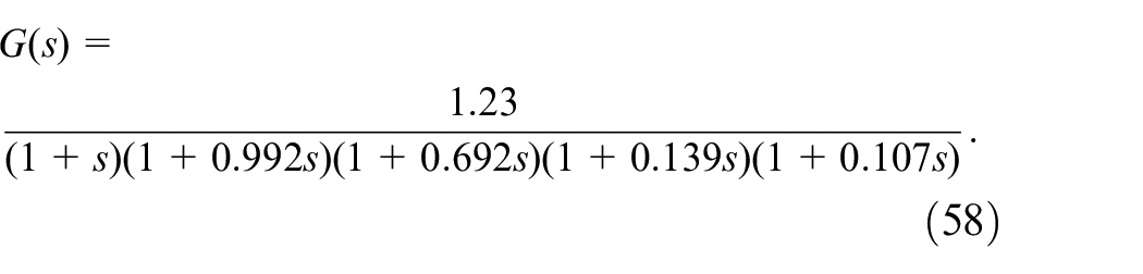
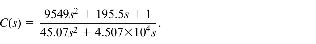
Select a set of optimized type-I controller parameters for the controller:
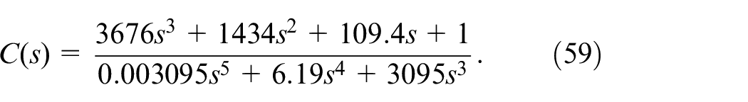
Select a set of optimized type-III controller parameters for the controller:
The adjustment time is
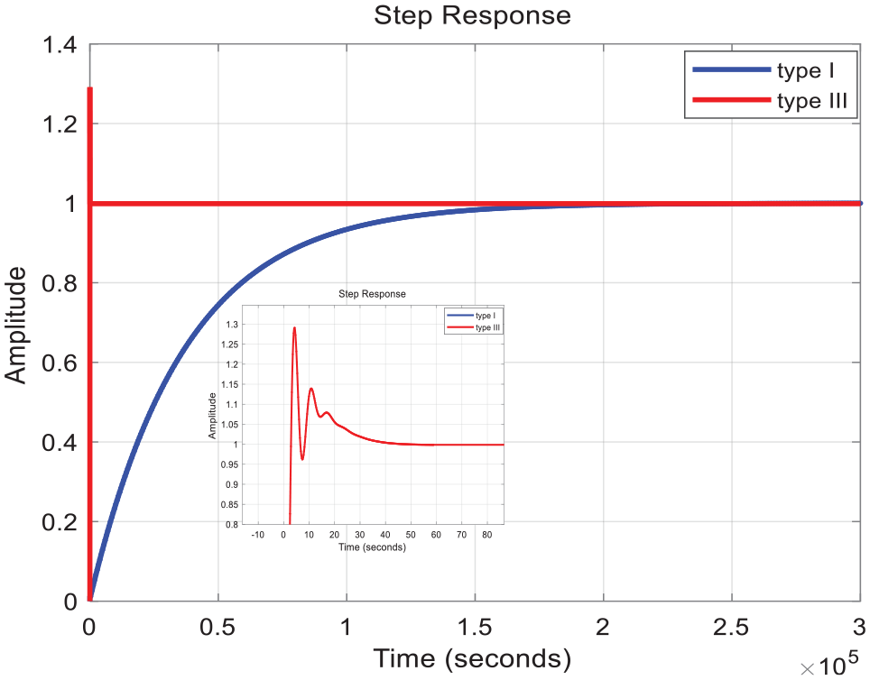
Comparison of step response.
The open-loop bode diagram and the closed-loop bode diagram of the system are shown in Figures 18 and 19. From Figure 18, we can get that the type-I system has a phase margin of 90.03º and an amplitude margin of 34.5 dB. The type-III system has a phase margin of 46.2º and an amplitude margin of 7.48 dB. As shown in Figure 19, the bandwidth of the type-I system is
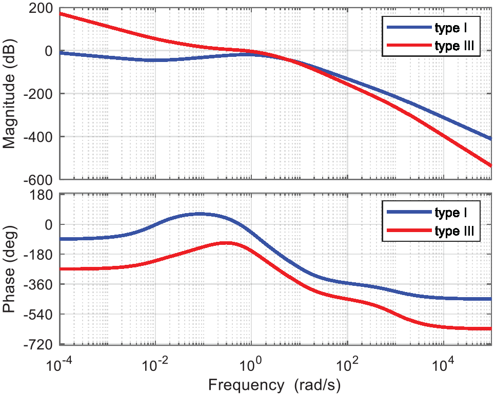
Comparison of open-loop bode diagrams.
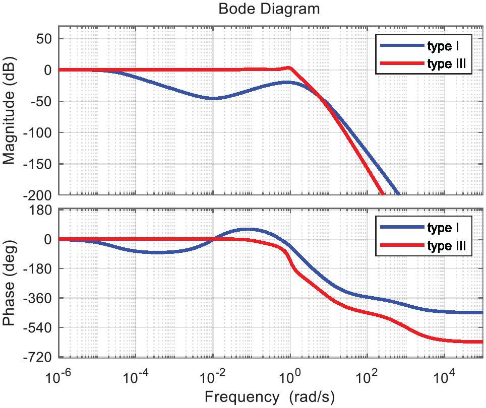
Comparison of closed-loop bode diagrams.
A comparison of the tracking of the ramp signal and the parabolic signal by the type-I and type-III systems is shown in Figure 20. From the comparison, the type-III system has significantly smaller tracking errors for both ramp and parabolic signals than the type-I system. So the type-III system can track signals in a short period of time, while the type-I system cannot track both signals effectively.
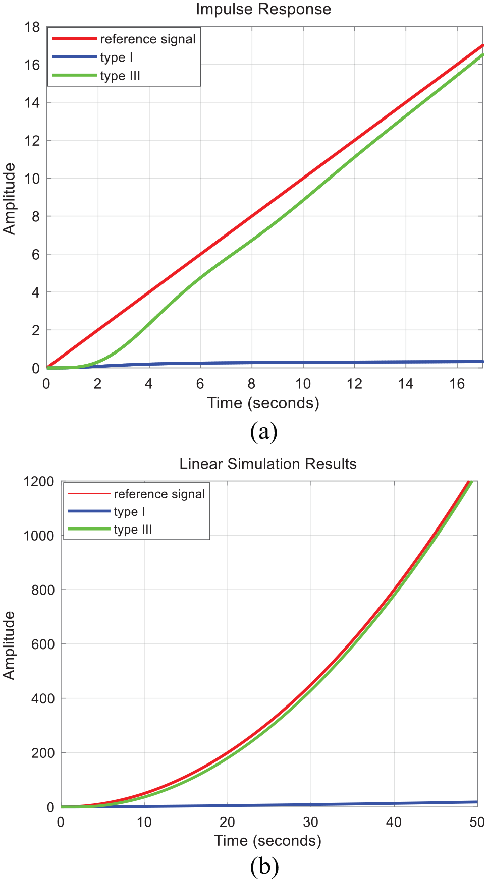
Comparison of signal tracking: (a) comparison of ramp signal tracking and (b) comparison of parabolic signal tracking.
Conclusion
In this article, we formulated the high-type intelligent control problem as a multi-objective problem. We considered the amplitude margin and phase margin as constraints to address the problem that the system is prone to instability in high-type systems. The multi-objective evolutionary algorithms are adopted to comprehensively optimize multiple indicators such as bandwidth and step response required by the control system. The experimental results show that the multi-objective high-type controller has better control in step response, robustness, and noise rejection capability in systems with delayed controlled objects and non-minimal phase, compared to controllers in the form of zero-dip pair elimination.
Footnotes
Acknowledgements
Dr Zhen Liangli (Institute of High Performance Computing) involved in the discussion of the idea for the paper and helped the preparation of the experiments, thanks to him for his contribution to this paper.
Declaration of conflicting interests
The author(s) declared no potential conflicts of interest with respect to the research, authorship, and/or publication of this article.
Funding
The author(s) disclosed receipt of the following financial support for the research, authorship, and/or publication of this article: This work was supported in part by the National Natural Science Foundation of China (Nos.1733012, No.61905253).