Sage Journals: Discover world-class research

Abstract

Serving as one of the core component, the excitation coil can exert remarkable influence on the output performance of giant magnetostrictive actuator (GMA) for electronic controlled fuel injector. In this paper, a multi-objective coil optimization scheme is proposed to balance the conflicting response speed and magnetic field intensity determined by the coil parameters. Firstly, a physics-based coil model is established for optimization, whose parameters can be directly calculated by the coil dimensions. Then, with the current response of the coil calculated, a multi-objective optimization framework is conducted attempting to get the selection guideline for the enameled wire diameter of the coil. The optimal choices exist when the outer diameter of the enameled wire falls in 0.9∼1.6 mm, and the inner/outer diameter ratio is relatively high. Finally, a series of experiments are conducted and the results indicate that the proposed model is able to accurately describe the current response throughout the operating frequencies, and the optimization scheme can provide a valuable roadmap to design coil for high performance GMA.

Keywords

physics-based modeling giant magnetostrictive actuator electronic controlled injector excitation coil model current response multi-objective optimization

Introduction

Gradually growing demand on fuel efficiency and pollutant emission of the internal combustion engine has resulted in rapid development of novel electronic controlled fuel injectors (ECI) based on smart materials including piezoelectric crystal, shape memory alloy, and giant magnetostrictive material (GMM), which possess some unique advantages over the traditional injectors.¹ Among the widely used smart materials, GMM is well-known for its excellent constitutive properties such as great output, significant efficiency, and high reliability.^2–4 Giant magnetostrictive actuator (GMA), designed utilizing GMM, inherits almost all the fantastic features of this material and becomes a promising device to drive the high-performance electronic controlled injectors.^5,6

Serving as the energy source of the magnetic field, the excitation coil plays an important role in determining the transient and steady state characteristics of GMA, like the response time, the magnetic field distribution, the maximum output, and the energy loss.^7,8 Therefore, it can be of paramount importance for researchers to conduct coil optimization, so that the optimal performance can be achieved when the structure of GMA is, to some extent, fixed. However, so far, only a few literatures have focused on this particular issue, and, meanwhile, many of them aim to obtain an evenly-distributed magnetic field along the axis of GMM rod.^9,10 For example, Gao et al. attempt to design and optimize the excitation coil parameters of GMA, expecting to acquire a highly-uniform magnetic field, and the uniformity rate can rise to 99.35% according to the simulation results in Ansoft.¹¹ Yang et al. investigate the influence of the coil length on the magnetic field distribution in GMA, and discover that it can generate quite evenly-distributed field while the coil possesses approximately the same length as the GMM rod.¹² In addition, Fan et al. propose optimization methods intended to minimize the power consumption utilizing shape factors, while Bai et al. design parallel coil with heat loss by decreasing the coupling inductance.^13,14 Several useful conclusions are drawn in these publications, which can provide some general roadmaps to conduct excitation coil design and optimization.^15,16

However, compared with other application conditions, GMA for ECI is a little different, for the magnetic field intensity uniformity and energy efficiency are usually not the most important indices to evaluate the output performance of this kind of actuator but the response speed.^17–19 Actually, although GMM can realize magneto-mechanical transition in several microseconds, the overall response speed of GMA is still not as quick as expected, due to the large inductance of the excitation coil, which can account for almost the entire response time of the actuator. Therefore, coils with smaller inductance are preferred while attempting to obtain faster response actuators. However, it should not be neglected that small inductance coil can lead to inadequate magnetic field, which may jeopardize the final output of the fuel injector. Based on the above analysis, how to balance the response speed and magnetic field intensity can be a challenging issue waiting to be addressed and this will be the main focus of this paper. To the best of the authors’ knowledge, only one published research focuses on this pending problem, which establishes a model to describe the relationship of coil turns, steady magnetic field intensity, and response time.²⁰ However, since this model is only suitable for the quasi-static excitations, and no direct conclusion on coil optimization is achieved, this research can hardly be useful in the practical optimization process.

When conducting coil optimization, it is necessary to employ voltage-current model to describe the coil current behaviors under different excitation signals. Unfortunately, modeling activities from the excitation voltage to the coil current are somewhat ignored in the present researches. And most of the GMA models begin with the coil current, making it hard to analyze the actual response time using these models.^21–24 According to the establishment process, the existing voltage-current models can be roughly divided into two types, namely, the statistical models and the physical models. The statistical models are established to mimic the dynamic properties of a system by different algorithms, which attract the researchers’ attention due to its high accuracy.^25,26 Different from the statistical models, the physical models are built based on certain physical mechanisms. Although the physical models are usually not as accurate as the statistical models especially in complex system cases, they are still widely used by scholars for they can explain the operating process of the target systems. Since the coil of GMA do not belong to the complex systems, the physical models are preferred, and the most popular one treats the coil as the series connection of a resistor and an inductor, which can describe the current using a first order differential equation.^1,27,28 This model exhibits good accuracy in low frequency ranges, but can cause unacceptable error while predicting the mid or high frequency responses. In this condition, some scholars propose several complicated models specially for the high frequency excitation.^7,29 However, some parameters of these models lack physical meanings, so it can be hard to use these models to guide coil optimization.

Given the above analysis, some attempts have been made in this work, and the contribution can be summarized as follows. Firstly, a fully physics-based optimization-oriented coil current model is established, where all the parameters can be directly computed by the structural dimensions of the excitation coil. Then, utilizing this model, the magnetic field intensity and the response time can be calculated, and a multi-objective optimization scheme is proposed to obtain the optimal coil design choice. Finally, a series of experiments under different excitation signals are conducted to validate the proposed coil model and the optimization method, and several conclusions are obtained to guide the structural design of the excitation coil.

The rest of this paper is outlined as follows: Structure of GMA for the fuel injector describes the basic structure and operating process of GMA for ECI; Physics-based model of the excitation coil establishes the physics-based voltage-current model used for optimization; Response analysis of the coil circuit model analyzes the current response of the excitation coil utilizing the proposed model; Parameter optimization of the excitation coil covers the proposed multi-objective optimization framework and achieves the optimization results; in Experimentation and model validation, experiments are conducted and the results are discussed; in Conclusions, some conclusions are provided concerning the optimal choice of the GMA coil design.

Structure of GMA for the fuel injector

Figure 1 shows the structure of GMA used for ECI, and its overall working principle can be expressed as follows: A rectangular voltage signal is usually exerted on the excitation coil while operating. When the signal turns to the high voltage, the response current will be generated in the coil and also form the excitation magnetic field along the coil axis. With the magnetic field, the GMM rod produces axial strain, pushing the nut and the output rod to move upward. After that, the ball valve fixed at the end of the rod opens upward, and the fuel injection can be realized. When the signal goes to the low voltage, the output rod can return under the action of spring. Then the ball valve closes, and the fuel injection activity stops.

Figure 1.

Structure of SGMA. (a) Sketch of SGMA (b) 3D model of SGMA. 1. Adjusting screw 2. Excitation coil 3. Coil skeleton 4. Giant magnetostrictive material rod 5. Gasket 6. Output rod 7. Sliding block 8. Shell 9. Nut 10. Spring 11 Head cover.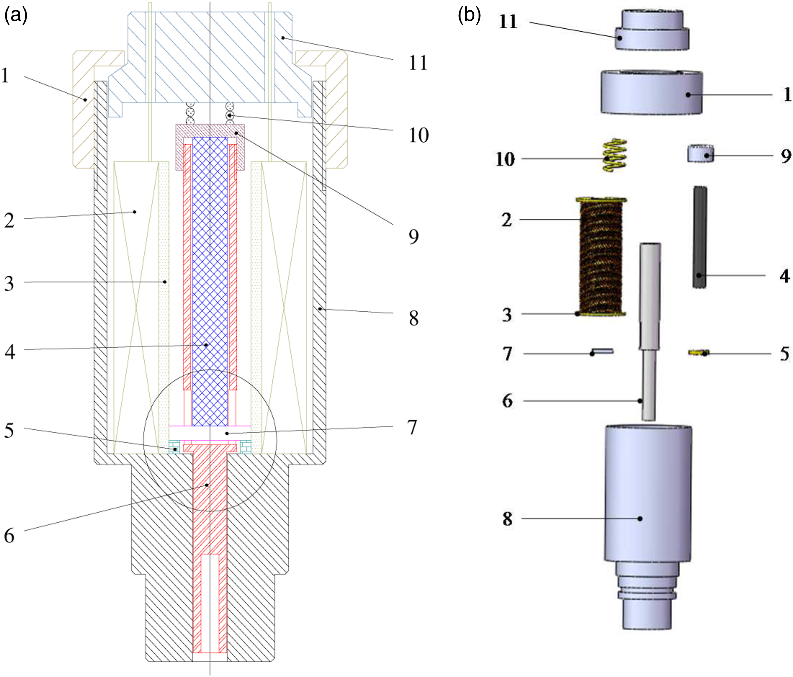

Physics-based model of the excitation coil

Model of the excitation coil dimensions

The structure and dimensions of the coil skeleton for GMA are shown in Figure 2, where d _h is the diameter of the enameled wire, d _l is the diameter of the copper core in the wire, c, c + 2b and a are the inner diameter, outer diameter, and effective length of the coil skeleton, respectively. According to the geometric relation, the average winding diameter of the coil can be represented by b + c.

Figure 2.

Dimension diagram of the excitation coil.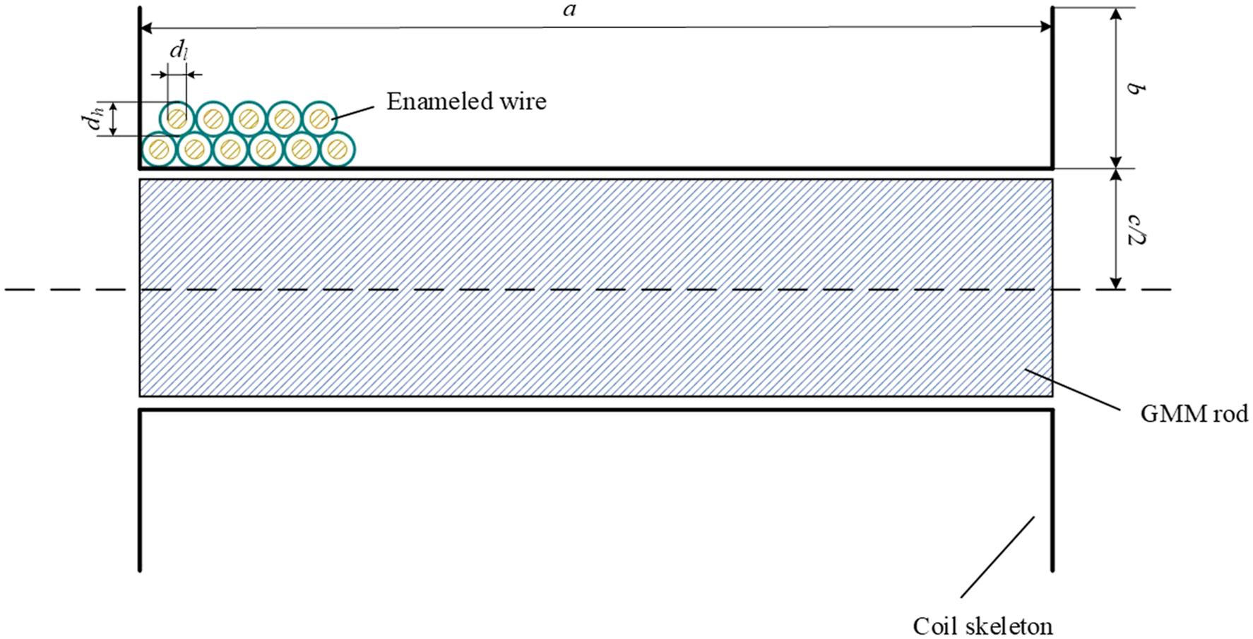

In the following part, some dimensional relationship is analyzed including that between the overall excitation coil frame dimensions and the enameled wire dimensions, as shown in Figure 3.

Figure 3.

Relationship between the coil skeleton dimensions and the enameled wire dimensions.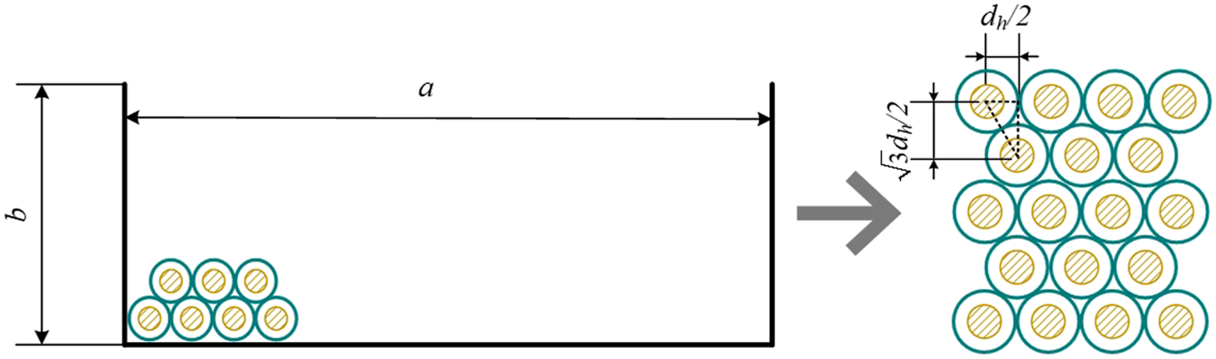

If the overall dimensions of the coil frame are fixed, the number of coil turns is mainly determined by the outer diameter of the enameled wire. And the layers in the axial and radial directions can be expressed as follows

n = ⌊ \frac{a}{d_{h}} ⌋

(1)

k = ⌊ \frac{2 (b - d_{h})}{\sqrt{3} d_{h}} + 1 ⌋

(2)

where

⌊ \cdot ⌋

represents rounding down to the nearest integer.

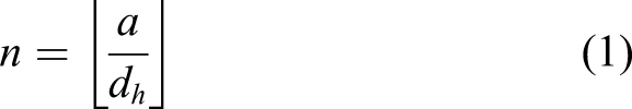
Then the total number of the coil N can be calculated as follows.

N = k n - ⌈ \frac{k}{2} ⌉

(3)

where

⌈ \cdot ⌉

represents rounding up to the nearest integer. Considering the winding clearance, a modification factor k _N is introduced, and equation (3) can be described as

N = k_{N} \frac{a b}{d_{h}^{2}}

(4)

Based on the above equations, the total winding length of the excitation coil can be computed as follows

l = k_{N} \frac{a b}{d_{h}^{2}} \cdot π \cdot \frac{c + c + 2 b}{2} = k_{N} π \frac{a b (b + c)}{d_{h}^{2}}

(5)

During the winding process, a deviation exists between the actual average coil radius and the theoretical one, which can result in a considerable gap between the actual wire length and the calculated value. Therefore, a length correction factor k _l is added to equation (5), and the total length of the excitation coil can be expressed as

l = k_{l} k_{N} \frac{a b}{d_{h}^{2}} \cdot π \cdot \frac{c + c + 2 b}{2} = k_{l} k_{N} π \frac{a b (b + c)}{d_{h}^{2}}

(6)

It should be noted that the value of k _l can be obtained by fitting a series of actual results with the same coil skeleton and different wire diameters.

Model of the excitation coil circuit

In order to study the voltage-current relationship of the excitation coil, it is necessary to establish an equivalent circuit model. For a multi-layer winding coil, it can be regarded as the series connection of an ideal resistor and an ideal inductor, and also parallel connection with an ideal capacitor, shown as Figure 4. Although this equivalent model is relatively simple, it matches the actual condition with acceptable accuracy. Especially when the signal frequency remains low, the steady and transient characteristics of the circuit can be well described.

Figure 4.

Equivalent circuit diagram of the excitation coil.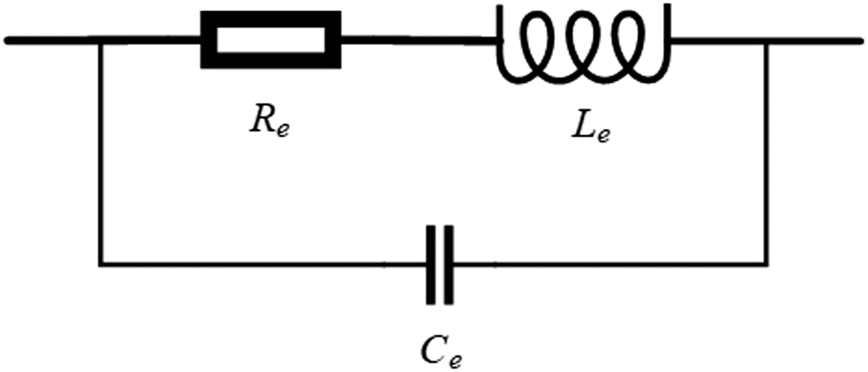

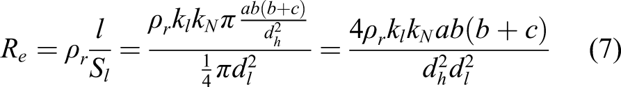
In the equivalent circuit, all the resistance, inductance, and capacitance can be calculated by the coil dimensions. The equivalent coil resistance R _e can be calculated by the following equation.

R_{e} = ρ_{r} \frac{l}{S_{l}} = \frac{ρ_{r} k_{l} k_{N} π \frac{a b (b + c)}{d_{h}^{2}}}{\frac{1}{4} π d_{l}^{2}} = \frac{4 ρ_{r} k_{l} k_{N} a b (b + c)}{d_{h}^{2} d_{l}^{2}}

(7)

where ρ _r denotes the resistivity of the enameled wire, and S _l denotes the cross-sectional area of the copper core in the enameled wire.

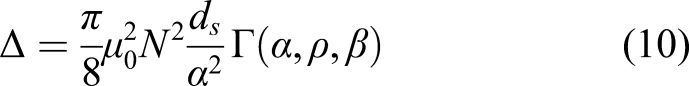
For the long coil whose skeleton length is larger than 0.75 times of the average diameter, the equivalent inductance L _e can be calculated by the following equation

L_{e} = L_{0} - Δ

(8)

where △ denotes the inductance correction value considering the radial thickness of the coil, L ₀ denotes the inductance of the solenoid with the same length and average diameter as the excitation coil, and the calculation equation can be expressed as

L_{0} = \frac{μ_{0}}{4 π} N^{2} d_{s} Φ_{s}

(9)

where μ ₀ denotes the air permeability, d _s denotes the diameter of the solenoid, whose value is b + c, and Φ_s denotes a constant related to the dimensions of the solenoid.

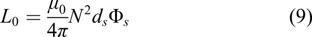
The inductance correction value can be calculated as

Δ = \frac{π}{8} μ_{0}^{2} N^{2} \frac{d_{s}}{α^{2}} Γ (α, ρ, β)

(10)

where α denotes the ratio of the coil length a to the average diameter b + c, ρ denotes the ratio of the coil radial thickness b to the average diameter b + c, Γ(α, ρ, β) denotes a function determined by α, ρ and β, and the calculation equation of β can be expressed as³⁰

β = \frac{1}{\sqrt{1 + 4 α^{2}}}

(11)

In the excitation coil, the interlayer capacitance should be treated as the dominant part of the equivalent capacitance. In order to make full use of the skeleton dimensions, the “U” type winding method is usually used in the GMA coil, shown as Figure 5.

Figure 5.

Schematic diagram of “U” type winding method.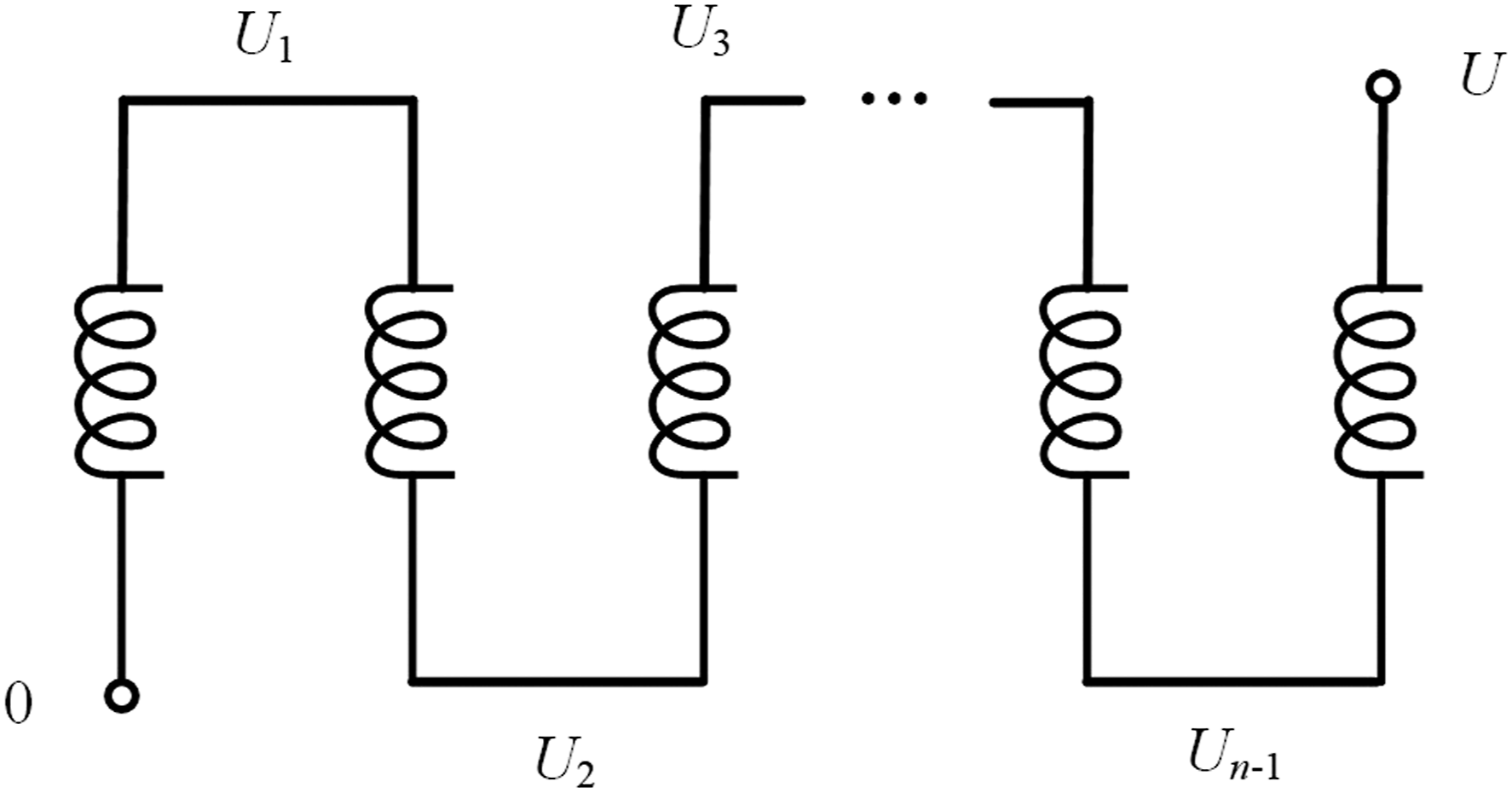

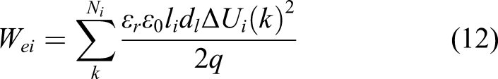
Considering the energy storage capacity in the capacitance element, the equivalent capacitance between two adjacent layers of the coil can be calculated from the stored electric energy. In the i ^th and (i + 1)^th layer of the coil, the calculation equation of the stored electric field energy can be computed as follows

W_{e i} = \sum_{k}^{N_{i}} \frac{ε_{r} ε_{0} l_{i} d_{l} Δ U_{i} {(k)}^{2}}{2 q}

(12)

where ε ₀ denotes the vacuum permittivity, ε _r denotes the relative permittivity of copper, l _i denotes the average turn length in the i ^th layer, U _i(k) denotes the electric potential difference of the k ^th turn between the i ^th and (i + 1)^th layer in the coil, which can be obtained by the ratio of the winding length of the i ^th layer to the total winding length of the coil, N _i denotes the number of coil turns in the i ^th layer, q denotes the distance between the corresponding turn in two adjacent layers, and the value can be represented by

\sqrt{3} d_{h} / 2

, shown in Figure 3.

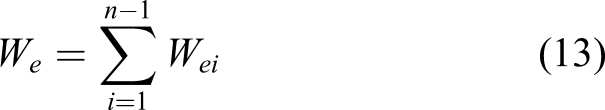
For the coil with n layers, the stored electric energy can be regarded as the sum of that in every two adjacent layers

W_{e} = \sum_{i = 1}^{n - 1} W_{e i}

(13)

where W _e denotes the total energy stored between adjacent layers.

Meanwhile, the stored electric energy can be expressed by the equivalent capacitance as follows

W_{e} = \frac{1}{2} C_{e} U^{2}

(14)

where C _e denotes the equivalent capacitance of the excitation coil, and U denotes the voltage exerted on the coil.

Response analysis of the coil circuit model

With the excitation coil circuit model established, further analysis on the performance of the excitation coil and influence of the coil parameters on its response characteristics under different operating conditions can be conducted. Therefore, the sinusoidal and square wave response properties of the circuit need to be considered.

When the excitation signal is employed on the coil, the response can be displayed as Figure 6, where the equivalent current in the coil can be represented by i(t).

Figure 6.

Diagram of the current response in the equivalent circuit.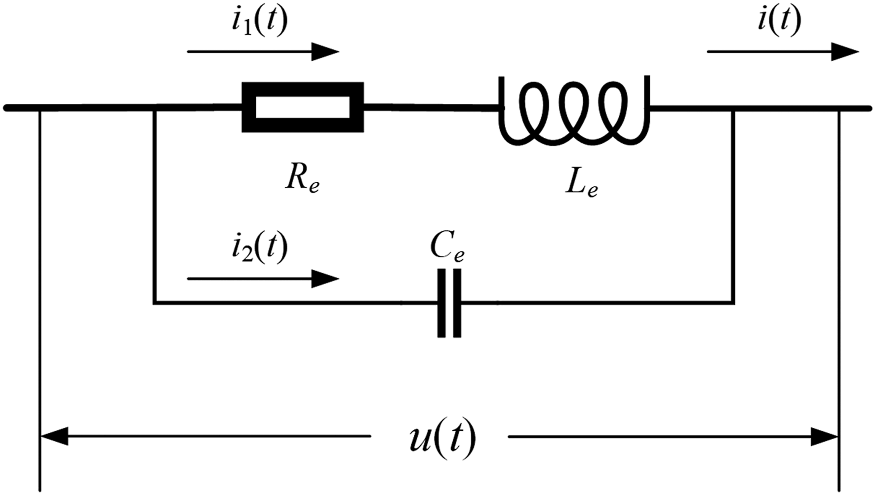

Based on the nodal current law, the total current in the excitation coil is equal to the sum of the current in each branch expressed as i(t) = i ₁(t) + i ₂(t).

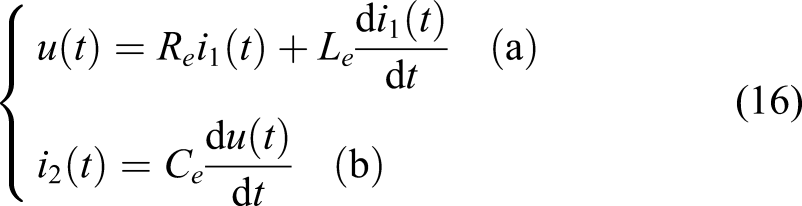
In addition, the voltage on each parallel branch remains equal, expressed by

u (t) = u_{C} (t) = u_{R} (t) + u_{L} (t)

(15)

where u(t) denotes the voltage on the excitation coil, u _c(t), u _R(t), and u _L(t) denotes the voltages exerted on the capacitance, resistance, and inductance in the equivalent circuit, respectively.

Considering the properties of the capacitance, resistance, and inductance, the above equations can be expressed as follows

{\begin{cases} u (t) = R_{e} i_{1} (t) + L_{e} \frac{d i_{1} (t)}{d t} (a) \\ i_{2} (t) = C_{e} \frac{d u (t)}{d t} (b) \end{cases}

(16)

where R _e, L _e and C _e represent the resistance, inductance, and capacitance of the equivalent circuit, respectively.

Response of the sinusoidal excitation

According to the theories of signal processing, the periodic excitation can be decomposed into a series of sinusoidal excitations. Therefore, analyzing the sinusoidal excitation response of the coil can be regarded as the premise and foundation for studying the response characteristics under other periodic excitations.

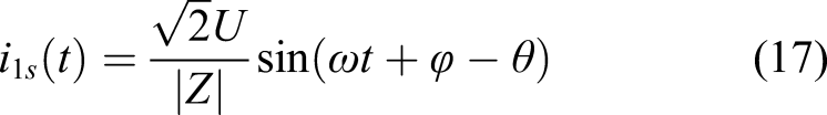
Assume that the excitation signal exerted on the coil can be written as $u (t) = U \sin (ω t + φ)$ , where ω denotes the angular frequency, and φ denotes the initial phase angle. In the resistance-inductance branch, the current response can be represented by the solution of equation (16a), and the expression is i ₁(t) = i _1s(t) + i ₁₀(t), where i _1s(t) and i ₁₀(t) are the steady and transient components of the circuit response, respectively.

The steady-state current can be expressed by a sinusoidal function as

i_{1 s} (t) = \frac{\sqrt{2} U}{| Z |} \sin (ω t + φ - θ)

(17)

where

| z | = \sqrt{R^{2} + {(ω L)}^{2}}

θ = \tan^{- 1} (\frac{ω L}{R})

After that, the transient component of the response current i ₁₀(t) is considered, which can be regarded as the particular solution of the homogeneous differential equation in equation (16a), represented by

i_{10} (t) = A e^{- \frac{R}{L} t}

(18)

where A is a constant, determined by the initial state of the coil. When the initial value of the coil current is i _10i,

A = i_{10 i} - U / | Z | \sin (φ - θ)

. In particular, if i _10i equals to 0, the coil is excited in the zero initial state, and

A = - U / | Z | \sin (φ - θ)

In the capacitance branch of the equivalent circuit, the current response is the solution of equation (16b), which can be expressed as

i_{2} (t) = ω C U \cos (ω t + φ)

(19)

Response of the square excitation

When the injector operates, the square signal should be applied on the excitation coil. In the ideal condition, the excitation signal should realize the voltage conversion at the time point t ₁. However, in the actual circuit, the devices cannot achieve ideal state, and the voltage is unable to realize sudden change, and a time interval ∆t is often obliged in this procedure. Therefore, the actual voltage signals on the excitation coil are shown as Figure 7, where U _h denotes the amplitude of the high voltage, U _l denotes the amplitude of the low voltage, and ∆t ₁, ∆t ₂, ∆t ₃, ∆t ₄ denote the voltage rising time, high voltage duration time, voltage declining time, and low voltage duration time respectively.

Figure 7.

Actual excitation waveform of the fuel injector.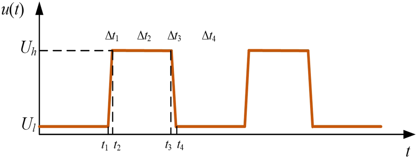

It can be discovered from Figure 7 that a complete excitation cycle can be divided into four stages. To obtain the current response of the system, it is necessary to analyze the characteristics of each excitation phase separately.

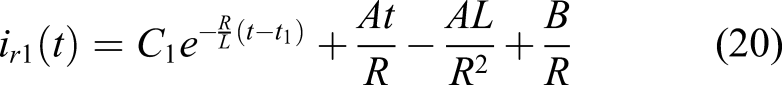
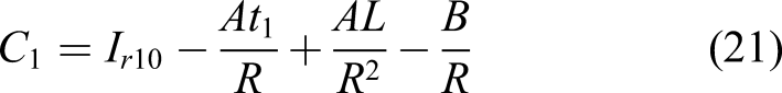
The excitation voltage in the rising phase can be expressed as u(t)=At+B. A and B are determined by the starting and ending time of voltage rising, and for the first excitation waveform in Figure 7, $A = \frac{u_{h} - u_{l}}{t_{2} - t_{1}}$ , $B = \frac{u_{l} t_{2} - u_{h} t_{1}}{t_{2} - t_{1}}$ .

Considering the rising voltage, the solution of the equation (16a) can be obtained, which can represent the current response in the resistance-inductance branch as follows

i_{r 1} (t) = C_{1} e^{- \frac{R}{L} (t - t_{1})} + \frac{A t}{R} - \frac{A L}{R^{2}} + \frac{B}{R}

(20)

where C ₁ denotes a constant, determined by the initial current value in this branch. Substituting it into the general solution, the value of C ₁ can be obtained as

C_{1} = I_{r 10} - \frac{A t_{1}}{R} + \frac{A L}{R^{2}} - \frac{B}{R}

(21)

where I _r10 denotes the initial current in the voltage rising phase.

For the capacitance branch, its current response is determined by the changing rate of the excitation voltage. The calculation equation can be expressed as $i_{r 2} (t) = C_{e} A$ .

When the voltage reaches the high level holding phase, the excitation voltage remains constant for some time, and the general solution of the current response in the resistance-inductance branch can be represented by $i_{h 1} (t) = C_{2} e^{- \frac{R}{L} (t - t_{2})} + U_{h} / R$ , where C ₂ is determined by the initial value of the branch current. In the capacitor branch, since the excitation voltage remains constant, the current in the capacitor always stays zero.

In the voltage declining phase, the excitation signal can also be expressed by u(t)=Et+F. E and F can be calculated by the starting and ending time of the rising voltage as $E = \frac{U_{l} - U_{h}}{t_{4} - t_{3}}$ , $F = \frac{U_{h} t_{4} - U_{l} t_{3}}{t_{4} - t_{3}}$ . Similarly, the current response of the resistance-inductance branch can be obtained as follows

i_{d 1} (t) = (I_{d 10} - \frac{E t_{3}}{R} + \frac{E L}{R^{2}} - \frac{F}{R}) e^{- \frac{R}{L} (t - t_{3})} + \frac{E t}{R} - \frac{E L}{R^{2}} + \frac{F}{R}

(22)

where i _d10 denotes the initial current in the voltage declining phase, namely, the final current in the high voltage holding phase. Considering the capacitance branch of the equivalent circuit, the calculation equation of the current response remains to be

i_{d 2} (t) = C_{e} E

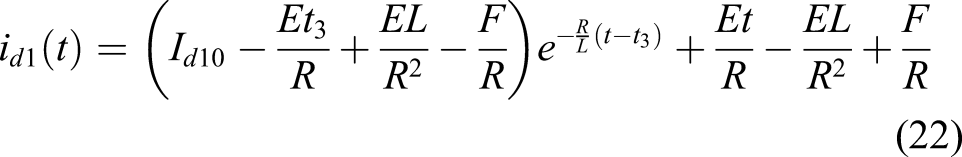
In the end, the low voltage holding phase is analyzed. During this period, the excitation voltage maintains at a constant value close to zero, and there is no current passing through the capacitance branch. In the resistance-inductance branch, the general solution of the current response is $i_{l 1} (t) = C_{4} e^{- \frac{R}{L} (t - t_{4})} + U_{l} / R$ . Similarly, the value of C ₄ can be determined by the final current in this branch excited by the previous phase.

From the above analysis, it can be seen that the current calculation in the capacitance branch tends to be relatively simple, which only depends on the voltage changing rate on the coil. In contrast, the resistance-inductance branch exhibits quite complex response characteristics, not only affected by the excitation voltage amplitude, but also closely related to the holding period of the high and low voltages. When the high voltage and low voltage holding phases in the excitation signal stay relatively long, the response current can reach the steady state value. In this condition, the initial branch current of the voltage rising and declining phases in each excitation cycle can be expressed as $U_{h} / R$ , and $U_{l} / R$ , respectively. On the contrary, when the holding phases are not long enough, the current will enter the next excitation phase while not reaching the steady state. The initial values of the branch current in the rising and declining phases need to be calculated iteratively based on the response of the previous phase.

Parameter optimization of the excitation coil

The response speed, regarded as the most important index to evaluate the performance of GMA, directly determines the fuel injection accuracy of the injector. The excitation coil contains large inductance, and will inevitably cause the lag of the response current and reduce the response speed of the system. In the design phase of the excitation coil, it is necessary to optimize the parameters aiming to shorten the response time. Meanwhile, to take full advantages of the large magnetostriction in GMM, improve the output displacement of the actuator, and reduce the heat generation problem of the device, the excitation coil should produce a relatively large magnetic field under small current condition. And in this way, the saturation magnetization of GMM can be ensured. Therefore, the parameter optimization of the excitation coil should surround the topic of improving the magnetic field intensity and reducing the current response time.

Analysis of the magnetic field intensity

Due to low permeability and poor magnetic conductivity, it is difficult for GMM to converge the magnetic field inside. Therefore, the closed magnetic circuit is often utilized in GMA structure design to improve the output efficiency. The magnetic circuit of GMA designed in this paper is shown in Figure 8(a). Based on the different materials and shapes, it is necessary to treat the components in GMA as different magnetic reluctance elements. The final equivalent magnetic circuit model can be displayed as Figure 8(b), where the magnetic field source is generated by the excitation coil.

Figure 8.

Diagram of the magnetic circuit. (a) Closed magnetic circuit in giant magnetostrictive actuator (b) Equivalent magnetic circuit model.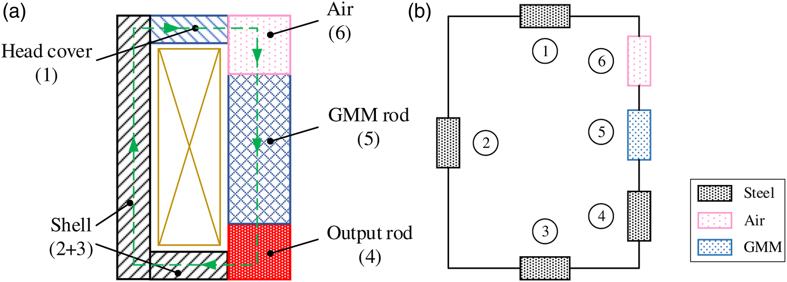

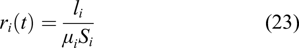
For the magnetic reluctance of each component in the equivalent magnetic circuit, the calculation equation can be expressed as

r_{i} (t) = \frac{l_{i}}{μ_{i} S_{i}}

(23)

where l _i, μ _i and S _i respectively denote the axial length, permeability and equivalent cross-sectional area of each component in the magnetic circuit.

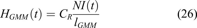
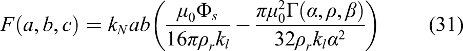
It should be noted that the permeability of GMM merely accounts for one thousandth of that of other components inside the magnetic circuit, indicating its magnetic reluctance far larger than those of other components. As for series connected magnetic circuit, the magnetic potential shared by each component always stays proportional to the magnetic reluctance of each component. Therefore, the magnetic potential generated by the excitation coil mostly exerts on the GMM rod, and the magnetic flux in the magnetic circuit can be calculated as

Φ_{M} (t) = \frac{N I (t)}{\sum r_{i}} \approx \frac{N I (t)}{r_{G M M}} = \frac{N I (t)}{l_{G M M} / (μ_{G M M} S_{G M M})}

(24)

where l _GMM, μ _GMM and S _GMM denote the length, permeability and cross-sectional area of the GMM rod respectively.

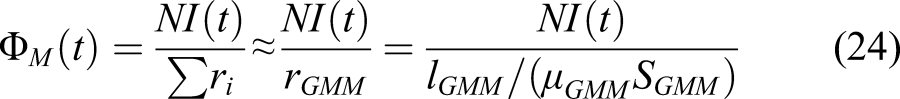
Then substitute $Φ_{M} (t) = μ_{G M M} H_{G M M} (t) S_{G M M}$ into equation (24), and the following equation can be obtained.

H_{G M M} (t) \approx \frac{N I (t)}{l_{G M M}}

(25)

where H _GMM(t) denotes the magnetic field intensity on the GMM rod. It should be noted that a correction coefficient C _R between 0∼1 is introduced into equation (25) to compensate for the calculation error caused by neglecting the magnetic reluctance of other components, and the final calculation equation of magnetic field can be expressed as

H_{G M M} (t) = C_{R} \frac{N I (t)}{l_{G M M}}

(26)

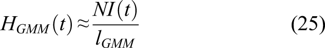
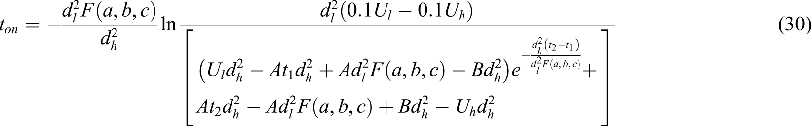
Analysis of the response time

Giant magnetostrictive actuator for ECI usually operates under the excitation of DC square wave, with high voltage opening, and low voltage returning. Therefore, it is very important to analyze the current response time on condition that the excitation voltage is switching from high-to-low or low-to-high. When the excitation frequency stays low, the coil current can reach steady state. Assume that ΔI denotes the difference between the high and low steady-state currents, and the time, when the current changing amplitude reaches 0.9ΔI, can be regarded as the characteristic parameter to evaluate the response speed of the coil, expressed as

t_{o n} = - \frac{L}{R} \ln \frac{(0.1 U_{l} - 0.1 U_{h})}{[(U_{l} - A t_{1} + \frac{A L}{R} - B) e^{- \frac{R}{L} (t_{2} - t_{1})} + A t_{2} - \frac{A L}{R} + B - U_{h}]}

(27)

t_{o f f} = - \frac{L}{R} \ln \frac{(0.1 U_{h} - 0.1 U_{l})}{[(U_{h} - C t_{3} + \frac{C L}{R} - D) e^{- \frac{R}{L} (t_{2} - t_{1})} + C t_{4} - \frac{C L}{R} + D - U_{l}]}

(28)

where, t _on and t _off denote the response time in the current rising and declining phase respectively. The derivation process of equation (27) is displayed in Appendix A, and equation (28) has a similar derivation process.

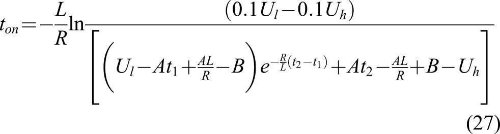
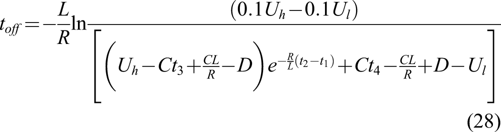
According to the circuit theories, the coil response time in DC square wave only relies on the circuit parameters, not influenced by the excitation frequency. Therefore, if the excitation frequency is high, the response current cannot reach steady state in the rising and declining phase. The response time can still be evaluated by equation (27) and (28).

Parameter optimization of the excitation coil

When the coil skeleton dimensions are determined, the steady-state magnetic field, and the response time of the coil are mainly affected by the winding turns, and the equivalent impedance, respectively. In order to achieve the optimal performance, these parameters need to be optimized. Based on the coil dimension model and coil circuit model, the turn number and equivalent impedance of the excitation coil can be determined by the inner and outer diameters of the enameled wire. Therefore, the final parameters to be optimized are set as these two. It should be noted that in practice, the inner diameter is supposed to be strictly smaller than the outer diameter, which needs to be taken as a constraint condition in optimization.

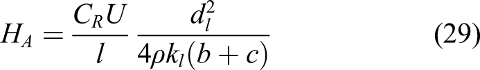
Substituting the circuit parameter expressions into equation (27) and (28), the magnetic field intensity and the response time can be calculated by the inner and outer diameters of the enameled wire as follows

H_{A} = \frac{C_{R} U}{l} \frac{d_{l}^{2}}{4 ρ k_{l} (b + c)}

(29)

t_{o n} = - \frac{d_{l}^{2} F (a, b, c)}{d_{h}^{2}} \ln \frac{d_{l}^{2} (0.1 U_{l} - 0.1 U_{h})}{[\begin{array}{l} (U_{l} d_{h}^{2} - A t_{1} d_{h}^{2} + A d_{l}^{2} F (a, b, c) - B d_{h}^{2}) e^{- \frac{d_{h}^{2} (t_{2} - t_{1})}{d_{l}^{2} F (a, b, c)}} + \\ A t_{2} d_{h}^{2} - A d_{l}^{2} F (a, b, c) + B d_{h}^{2} - U_{h} d_{h}^{2} \end{array}]}

(30)

where F(a, b, c) denotes a function determined by coil dimensional parameters a, b and c, and the expression can be displayed as follows

F (a, b, c) = k_{N} a b (\frac{μ_{0} Φ_{s}}{16 π ρ_{r} k_{l}} - \frac{π μ_{0}^{2} Γ (α, ρ, β)}{32 ρ_{r} k_{l} α^{2}})

(31)

where the meaning of the parameters are the same as those in the above sections. As is described in Model of the excitation coil circuit, α, β, and ρ are all defined by a, b, and c. The derivation process of equation (30) is displayed in detail in Appendix B.

The steady-state magnetic field intensity and the response time in different inner and outer wire diameters can be exhibited in Figures 9 and 10. Since the inner diameter should be smaller than the outer one, the curved surfaces in these two figures only reserve half of the complete surface.

Figure 9.

Relationship between coil parameters and steady magnetic field.

Figure 10.

Relationship between coil parameters and response time.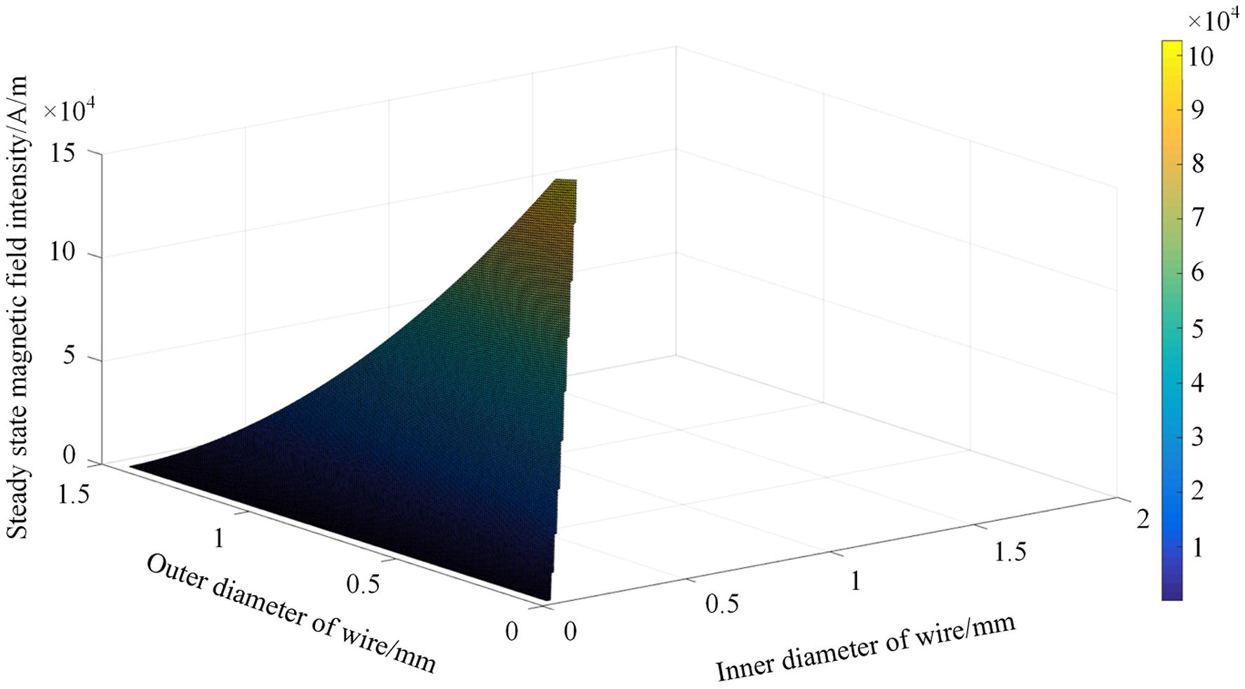

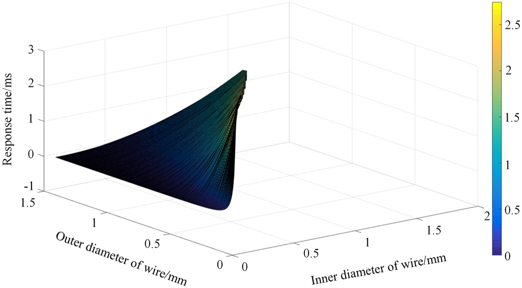
It should be noted that the insulating layer of the enameled wire is usually small compared to the wire diameter. And the curve features near the diagonal position in Figures 9 and 10 should be highlighted. It can be discovered that with the increase of the inner and outer diameters of the wire, the steady-state magnetic field intensity goes up gradually, but meanwhile the response speed of the coil tend to decrease. Therefore, these two performance indicators have mutual constraints in the optimization process, and it is necessary to use multi-objective optimization method to obtain the optimal solution of coil parameters.

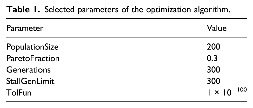
The embedded function in MATLAB, gamultiobj, is developed based on the genetic algorithm (GA), able to realize multi-objective optimization under certain constraints. The algorithm inherits the advantages of the traditional GA, including strong global searching ability, good robustness, and high efficiency. According to the above analysis, the objective function and constraint conditions of multi-objective optimization can be expressed as

\begin{array}{l} \min {\begin{array}{l} f_{1} (d_{h}, d_{l}) = - H_{A} \\ f_{2} (d_{h}, d_{l}) = t_{o n} \end{array} \\ s . t . {\begin{array}{l} d_{h} \geq 0 \\ d_{l} \geq 0 \\ d_{h} - d_{l} > ε \\ d_{h} - d_{l} \leq 8 \times 10^{- 5} \end{array} \end{array}

(32)

where ε denotes a given sufficiently small number.

Since the response time of the excitation coil only falls in microseconds, the objective function f ₂ amplifies 1000 times in the optimization process to avoid algorithm failure. And the parameters of optimization algorithm are selected as Table 1. Among these parameters, TolFun is set as an extremely small value to guarantee the accuracy of the output results. ParetoFraction and StallGenLimit are chosen based on the default values recommended by Matlab, with PopulationSize and Generations determined by a series of trial simulations. The values of these two parameters are increased step by step from the default values. When the optimization results become stable, it is considered that the values are the best ones with least computational load.

Table 1.

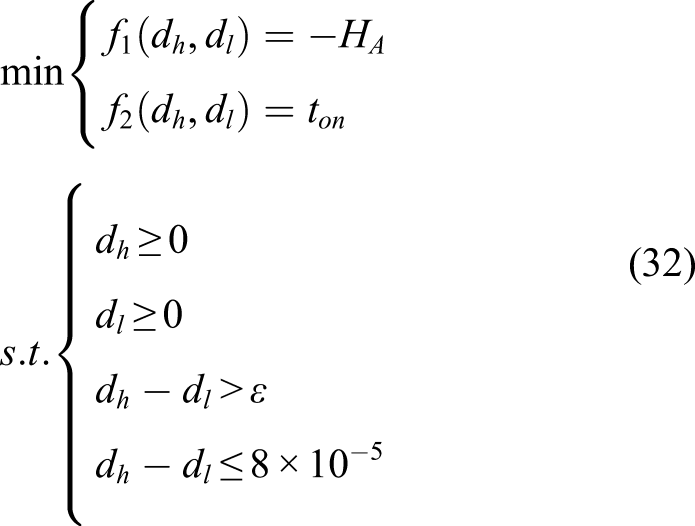
Selected parameters of the optimization algorithm.

Parameter	Value
PopulationSize	200
ParetoFraction	0.3
Generations	300
StallGenLimit	300
TolFun	1 × 10⁻¹⁰⁰

Conducting the optimization algorithm, 60 Pareto front solutions are obtained. The distribution of Pareto front individuals is shown as Figure 11.

Figure 11.

Pareto solution distribution after optimization.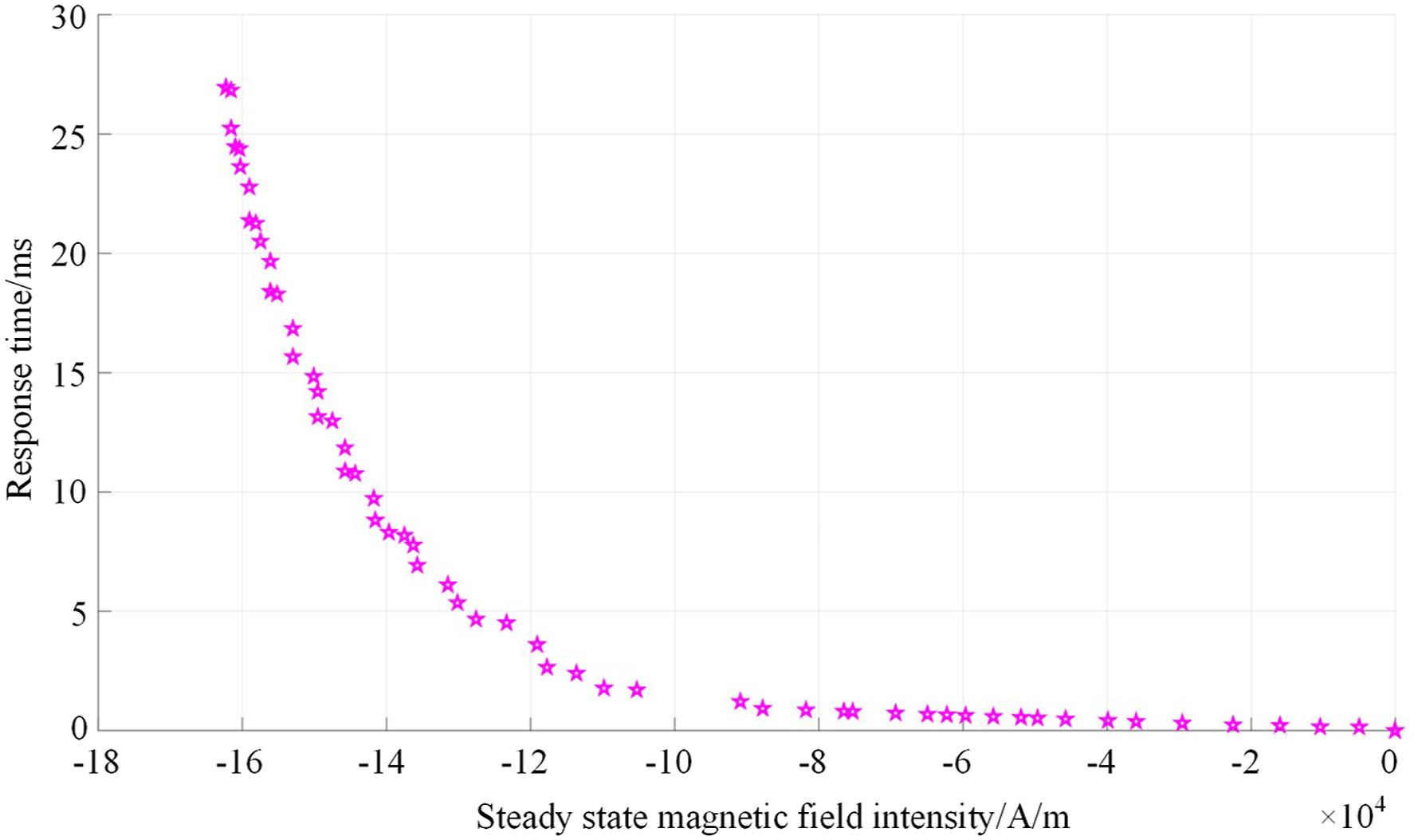

Since the Pareto front is defined as the set of non-dominated solutions, where each objective is considered as equally good, the best choice among them fitting the coil optimization case needs to be determined using other criteria. Similar with other ferromagnetic materials, GMM experiences saturation when it is excited by the magnetic field, which indicates that the magnetostriction can hardly further increase with the external magnetic field intensity larger than a certain value. Therefore, a best choice can be the Pareto solutions with the fastest response speed satisfying the magnetic field intensity requirements. To conduct the selection process, a searching algorithm is established as follows:

Step.1

Calculate the magnetic field intensity of all the Pareto solutions, and sort the Pareto solutions.

Step.2

Obtain the H-M (magnetic field intensity-magnetization intensity) curve of the utilized GMM, and determine the saturation threshold.

Step.3

Reserve the Pareto solutions whose magnetic field intensity larger than the threshold, and sort them according to the response time.

Step.4

Choose the Pareto solutions with or close to the shortest response time.

Employing this method, the balanced solutions can be determined based on the magnetic field intensity and response time. In this paper, the optimization choices exist when the outer diameters of the enameled wire fall in 0.9∼1.6 mm, and the inner/outer diameter ratio is relatively high, which can be a guideline for coil optimization in GMA for ECI.

To describe the parameter optimization procedure of the excitation coil in detail, a flowchart is displayed as Figure 12.

As the magnetic field intensity and the response time can be directly calculated by the coil dimensions using analytical expressions, almost all model complexity exists in the MATLAB function gamultiobj, and the value is Ο(GMN ²), where G denotes the iteration generations, M denotes the objective numbers, and N denotes the population size.

Figure 12.

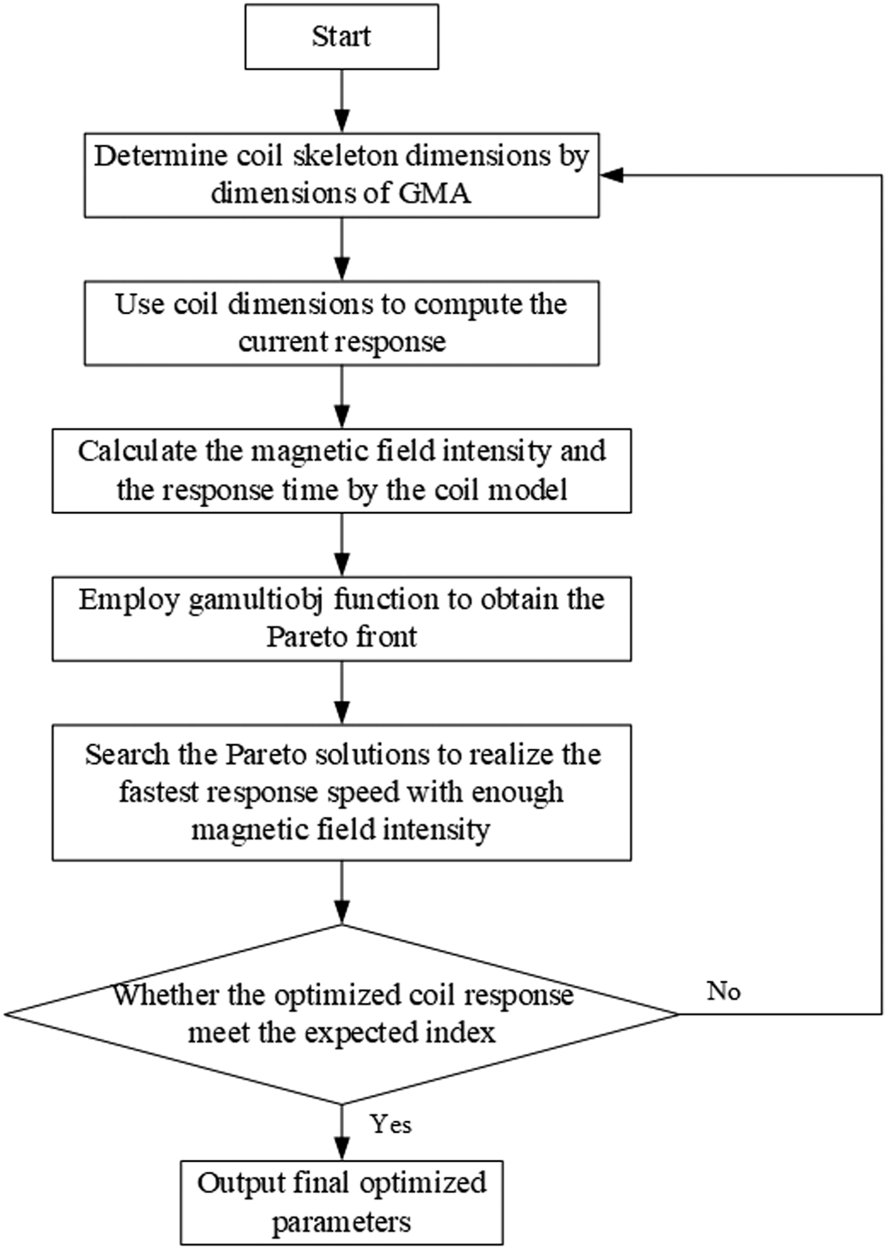
Parameter optimization procedure of the excitation coil.

Experimentation and model validation

In order to validate the coil model and parameter optimization method proposed in this paper, the excitation coil performance experiments are conducted utilizing the GMA testing system, shown as Figure 13. There are several essential parts constituting the system and its operating process can be described as follows: The digital oscilloscope, as the core of the system, is used to generate different signal waveforms provided by the master computer, and the signals are exerted on the coil after enlarged by the power amplifier. Then the response current generates in the coil, forming an excitation magnetic field in the three-dimensional space and driving the GMM rod to produce magnetostriction. The current clamp is used to collect the current in the coil, and the current signal together with the power amplifier voltage is input into the digital oscilloscope, which can be displayed on the master computer after processed by the data acquisition software.

Figure 13.

Experimental system for coil performance testing.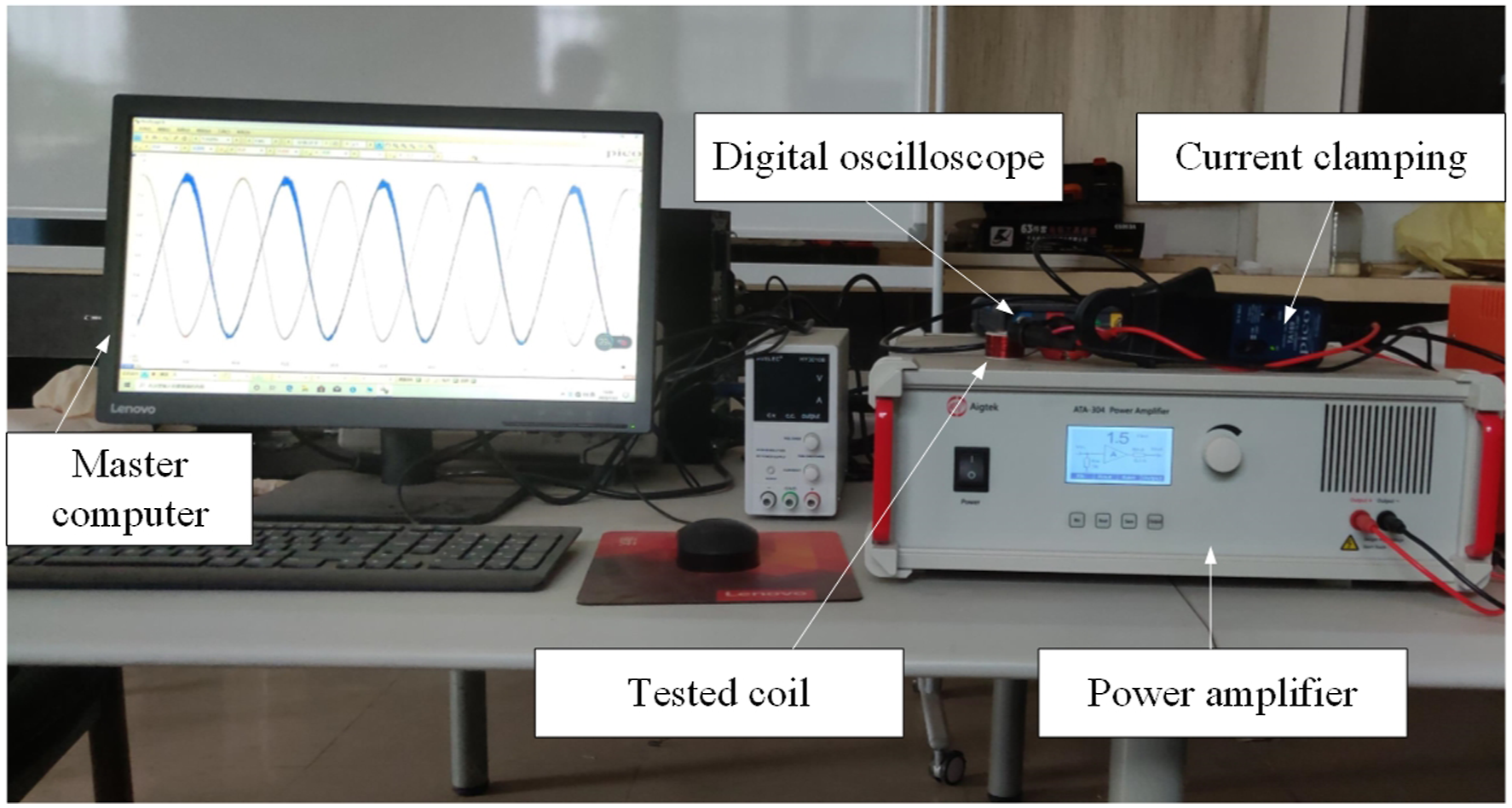

Validation of the coil model

With the parameters of the coil skeleton determined, several excitation coil prototypes are fabricated using enameled wire in different diameters. As shown in Figure 14, the diameters of the enameled wire for Coils 1∼6 are 0.29 mm, 0.38 mm, 0.49 mm, 0.59 mm, 0.69 mm and 0.8 mm respectively.

Figure 14.

Coil 1∼6 with different diameters of enameled wire.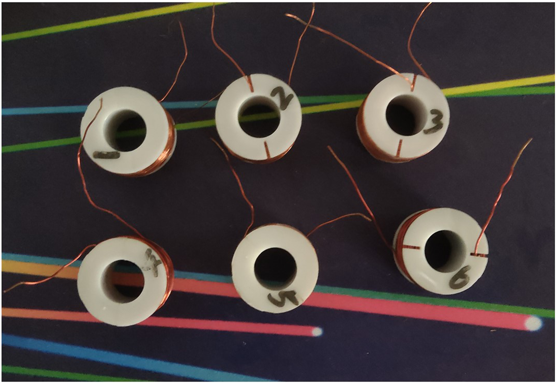

From equation (4), it can be discovered that with the dimensions of the coil skeleton fixed, the turn number of the coil should be linearly related to the reciprocal of the wire diameter square. Therefore, the relationship between them is plotted, and can be shown as Figure 15.

Figure 15.

Relationship between reciprocal of the wire diameter square and the number of coil turns.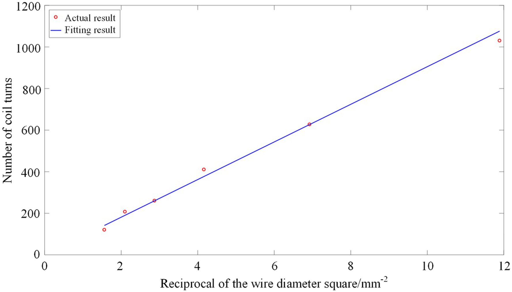

It can be seen that there is a clear linear relationship between the actual coil turns and the reciprocals of wire diameter square. In addition, the actual values distribute evenly on both sides of the fitting line, which proves the accuracy of the coil model. The maximum error occurs when the wire diameter is 0.29 mm, and the difference between the actual value and the fitting value is 46. In this case, the wire diameter is relatively small, and the clearance between two adjacent turns can be inevitable and more difficult to control compared with large diameter wire cases.

Validation of the coil circuit model

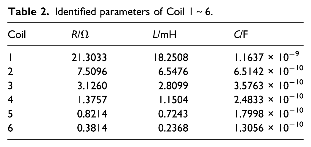
In the practical experimental conditions, it is not feasible and accurate enough to measure the resistance, inductance, and capacitance of the equivalent circuit directly. Therefore, in this paper, the component values in the equivalent circuit are obtained by identifying the modulus and phase angle of the measured impedance. For the circuit diagram shown as Figure 6, the impedance calculation equation can be expressed as follows.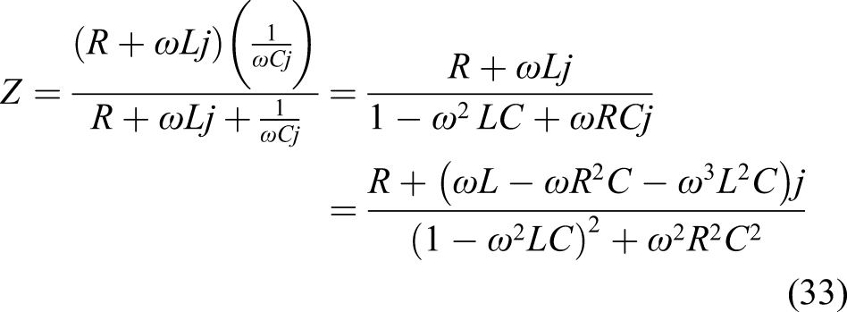

Z = \frac{(R + ω L j) (\frac{1}{ω C j})}{R + ω L j + \frac{1}{ω C j}} = \frac{R + ω L j}{1 - ω^{2} L C + ω R C j} = \frac{R + (ω L - ω R^{2} C - ω^{3} L^{2} C) j}{{(1 - ω^{2} L C)}^{2} + ω^{2} R^{2} C^{2}}

(33)

Then modulus and phase angle of impedance can be computed as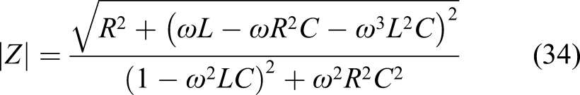

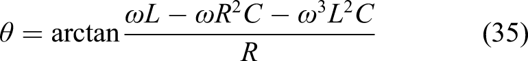
| Z | = \frac{\sqrt{R^{2} + {(ω L - ω R^{2} C - ω^{3} L^{2} C)}^{2}}}{{(1 - ω^{2} L C)}^{2} + ω^{2} R^{2} C^{2}}

(34)

θ = arctan \frac{ω L - ω R^{2} C - ω^{3} L^{2} C}{R}

(35)

Using the equations above, particle swarm optimization algorithm is used to conduct parameter identification, due to its high precision. And the identification values of Coil 1∼6 are obtained shown as Table 2.

Table 2.

Identified parameters of Coil 1∼6.

Coil	R/Ω	L/mH	C/F
1	21.3033	18.2508	1.1637 × 10⁻⁹
2	7.5096	6.5476	6.5142 × 10⁻¹⁰
3	3.1260	2.8099	3.5763 × 10⁻¹⁰
4	1.3757	1.1504	2.4833 × 10⁻¹⁰
5	0.8214	0.7243	1.7998 × 10⁻¹⁰
6	0.3814	0.2368	1.3056 × 10⁻¹⁰

Substituting the identified parameters into equation (6), the relationship between the modification factor k _l and the wire diameter can be obtained, shown as Figure 16.

Figure 16.

Values of k _l in different enameled diameters.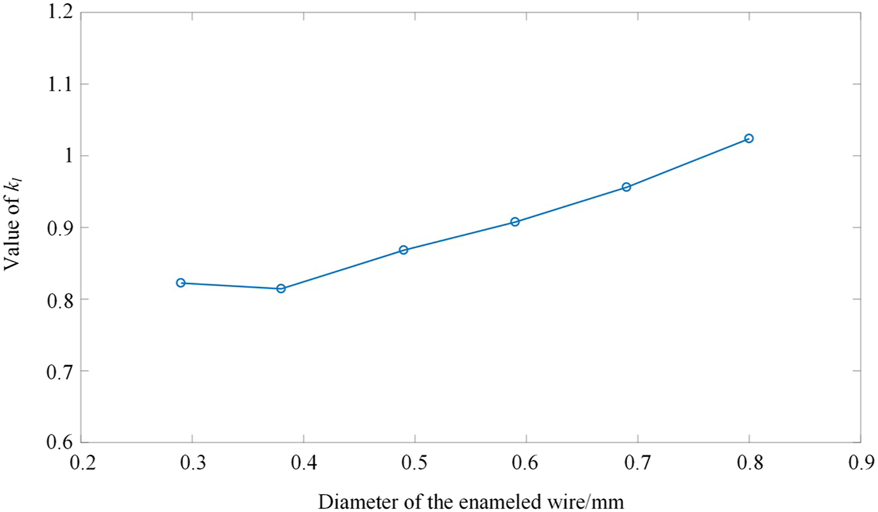

From Figure 16, it can be discovered that while the wire diameter is larger than 0.4 mm, the value of k _l keeps almost linear with the wire diameter; however, when the wire diameter goes down less than 0.4 mm, k _l nearly remains unchanged. Therefore, the value of k _l can be expressed in the form of piecewise function as follows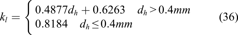

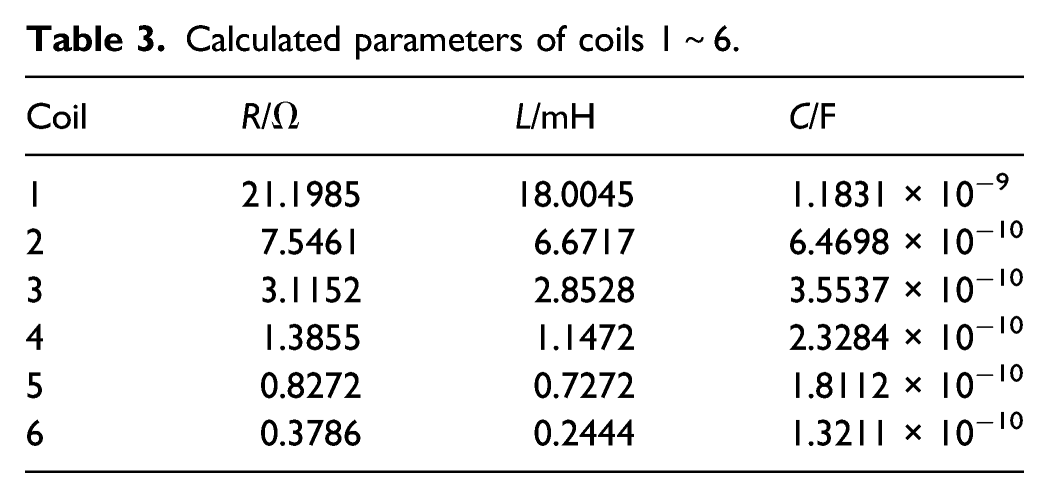
k_{l} = {\begin{cases} 0.4877 d_{h} + 0.6263 d_{h} > 0.4 m m \\ 0.8184 d_{h} \leq 0.4 m m \end{cases}

(36)

Based on the aforementioned analysis, the calculated values of resistance, inductance and capacitance in the equivalent circuit can be obtained, as shown in Table 3. And the corresponding relative errors are plotted in Figure 17.

Table 3.

Calculated parameters of coils 1∼6.

Coil	R/Ω	L/mH	C/F
1	21.1985	18.0045	1.1831 × 10⁻⁹
2	7.5461	6.6717	6.4698 × 10⁻¹⁰
3	3.1152	2.8528	3.5537 × 10⁻¹⁰
4	1.3855	1.1472	2.3284 × 10⁻¹⁰
5	0.8272	0.7272	1.8112 × 10⁻¹⁰
6	0.3786	0.2444	1.3211 × 10⁻¹⁰

Figure 17.

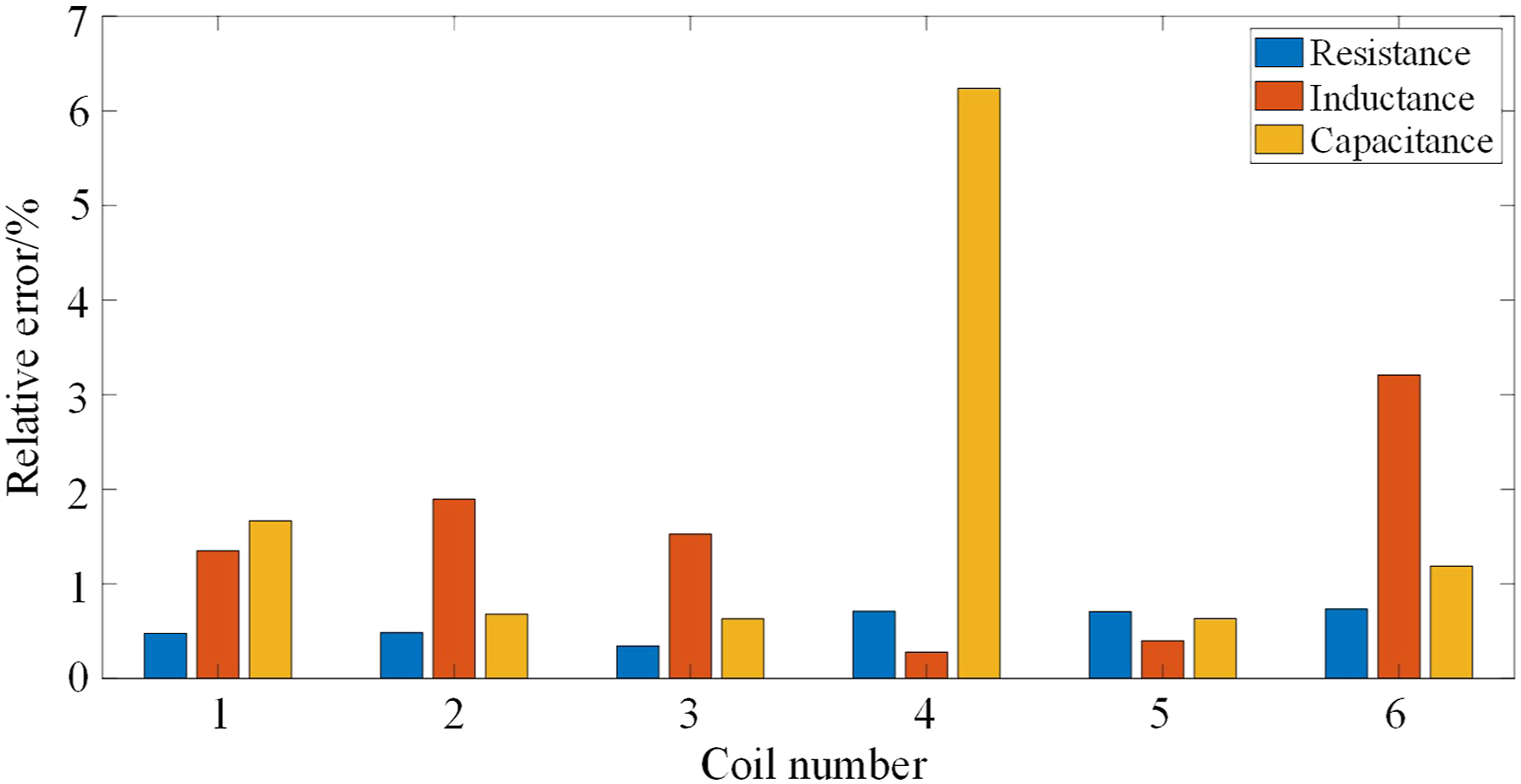
Relative errors between calculated parameters and identified parameters.

From Table 3 and Figure 17, it can be detected that most of the calculated values locate quite close to the identified ones, indicating that the established model can well describe the properties of the excitation coil. The maximum relative error occurs while calculating capacitance, whose value is around 6.2%. The explanation of this deviation can be described as: In the equivalent circuit, the capacitance is comparatively small, and does not influence the coil performance too much. Therefore, it can be difficult for the identification algorithm to obtain the exact value of the capacitance.

To further verify the equivalent circuit model and parameter calculation method proposed in this paper, the calculated impedance is compared with the measured one. The results are shown in Figures 18 and 19.

Figure 18.

Comparison of calculated and experimental modulus of impedance in different excitation frequencies.

Figure 19.

Comparison of calculated and experimental phase angle of impedance in different excitation frequencies.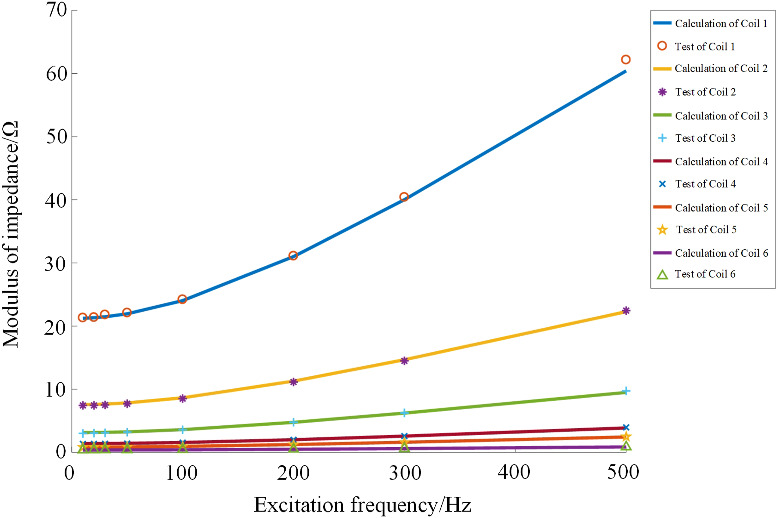

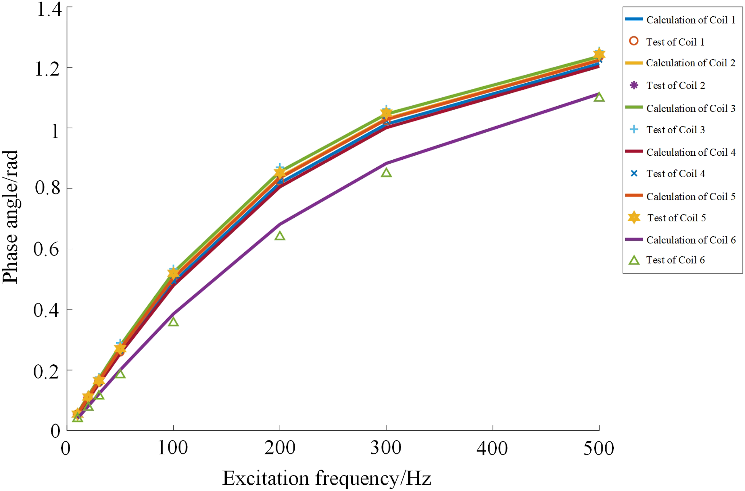
It can be seen that the calculated values agree well with the measured modulus and phase angles of the coil impedance throughout the operating frequency range. The largest relative error, with the value being 8.41%, emerges while computing the phase angle of Coil 6, which indicates that the coil equivalent circuit model and parameter calculation method proposed in this paper possesses relatively high accuracy.

Validation of the response current model

In order to further analyze the excitation coil model and check its ability to describe the transient current response properties, sinusoidal and square wave excitation experiments are conducted. The experimental results and the corresponding errors with the calculated ones in sinusoidal excitation are shown as Figures 20 and 21.

Figure 20.

Current response of Coil 1 under sinusoidal excitation at different frequencies (a) 10 Hz, (b) 100 Hz, (c) 500 Hz.

Figure 21.

Current response of different coils under sinusoidal excitation at the same frequency. (a) Coil 4 and (b) Coil 6.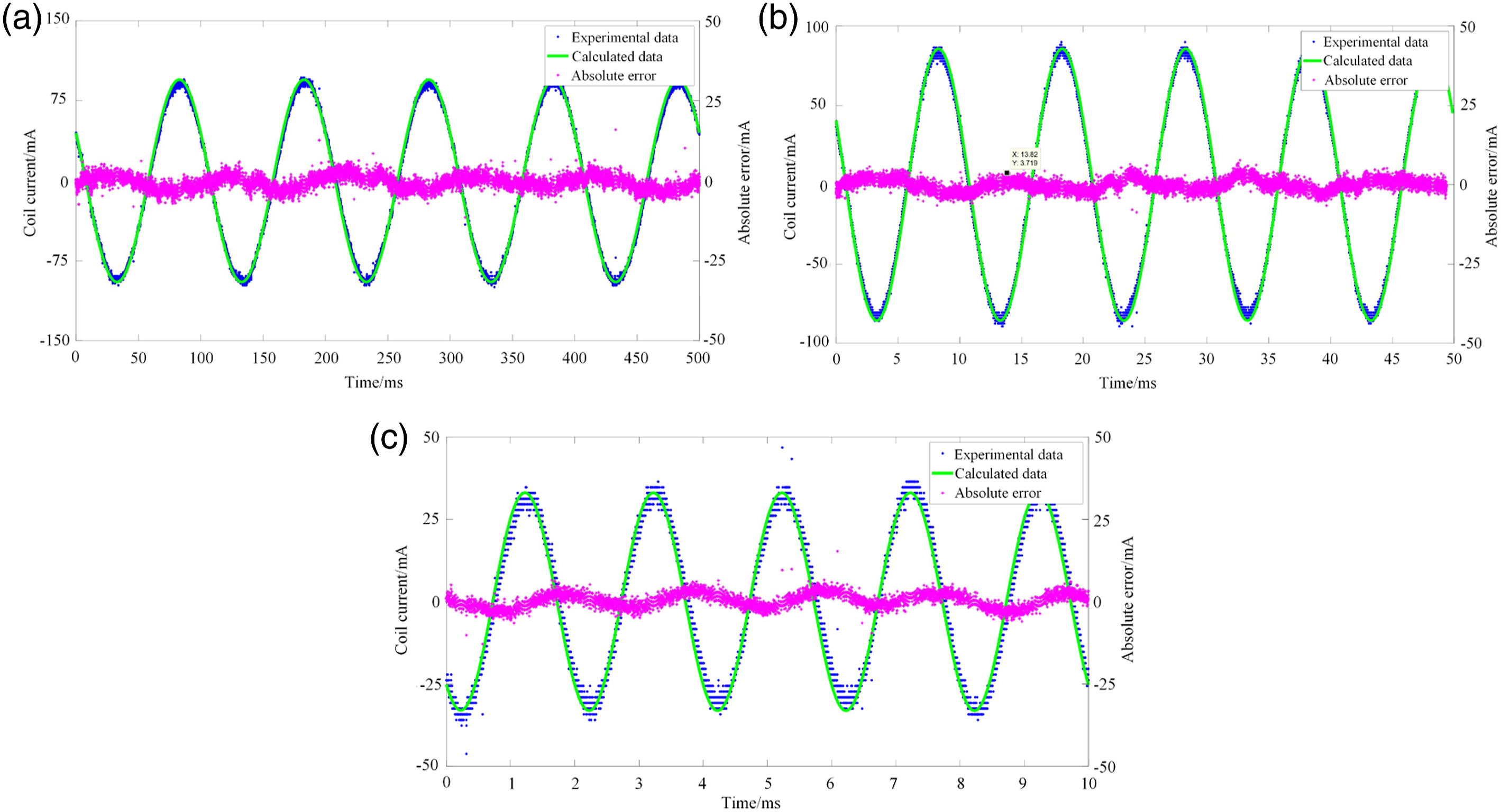

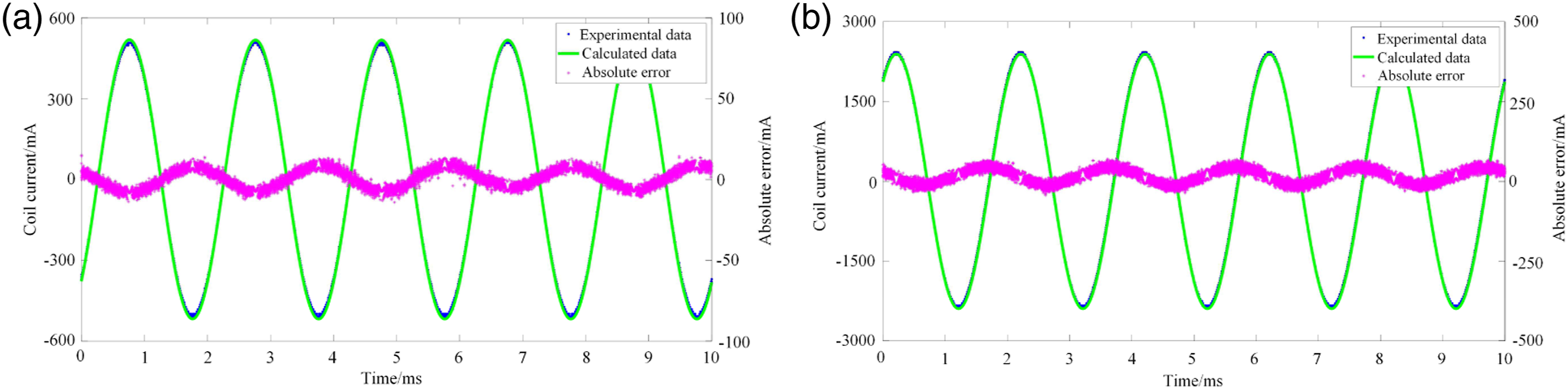
From Figures 20 and 21, it can be seen that under sinusoidal excitation, the calculated results of the model remains in good agreement with the experimental ones, and the model can accurately describe both the amplitude and phase of the sinusoidal response current. From the error curve, it can be discovered that the absolute errors between experimental data and model data always stay in low level. Except some special points, the relative errors also keep below 8%, with most of them smaller than 5%. Besides, to further analyze the difference between the model results and experimental results, root mean square error (RMSE) calculation is conducted. As for the cases shown in Figure 20, the RMSEs in three frequencies are 2.24 mA, 1.88 mA, and 2.20 mA, respectively, which can be regarded as very small values compared with the current amplitudes. And the calculated RMSEs in Figure 21 are 5.85 mA and 28.04 mA, which are larger than those mentioned above, and can be caused by the testing errors of the current clamp in higher measurement range. However, considering the currents in Coil 4 and Coil 6, the RMSEs still indicate good accuracy of the model.

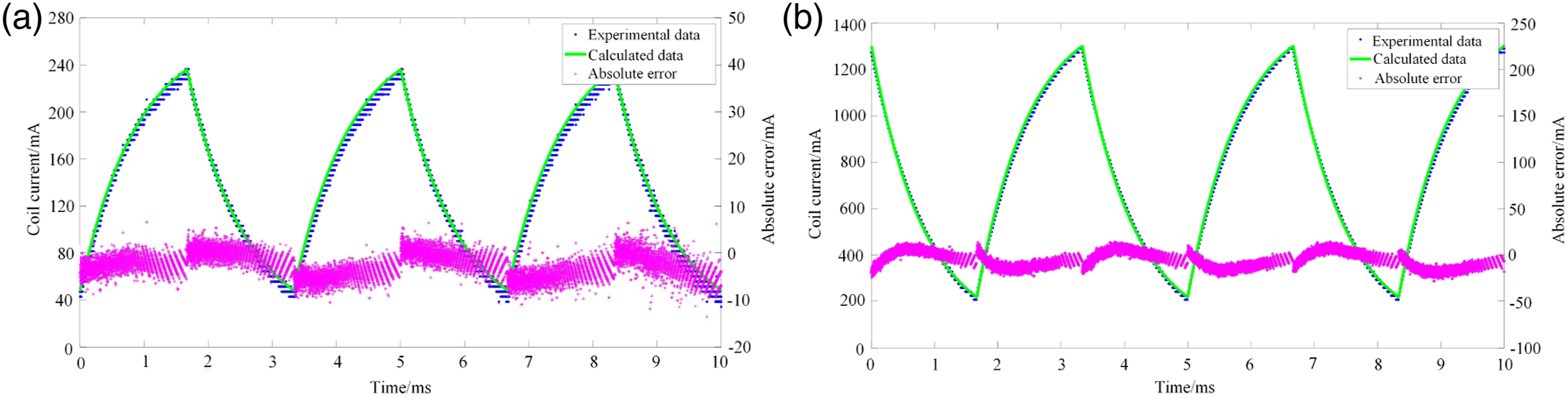
In addition to sinusoidal excitation, a series of DC square wave signals in different frequencies are applied on Coil 1 as well, and the current response is shown in Figure 22. It can be discovered that under different frequencies, the model calculation results coincide with the experimental results well, and the model can maintain high accuracy in describing the basic characteristics of the current response, like the upper and lower limits, rising and declining time and changing trend. According to the error curves in the figures, it can be seen that the absolute errors are even smaller than those under the sinusoidal excitations. The computed RMSEs in the provided three frequencies are 1.79 mA, 1.78 mA, and 1.81 mA, respectively, indicating its suitability for the square excitations. Figure 23 shows the current response curves of Coil 2 and Coil 4 with the excitation frequency of 300 Hz, and the RMSEs are 3.68 mA and 9.90 mA, respectively. Combined with the experimental results of Coil 1, the model exhibits strong adaptability for coils in different dimensions, and can accurately predict the square wave excitation experimental results of coils with different dimensional parameters.

Figure 22.

Current response of Coil 1 under square wave excitation at different frequencies. (a) 20 Hz, (b) 50 Hz, (c) 300 Hz.

Figure 23.

Current response of different coils under square wave excitation at the same frequency. (a) Coil 2 and (b) Coil 4.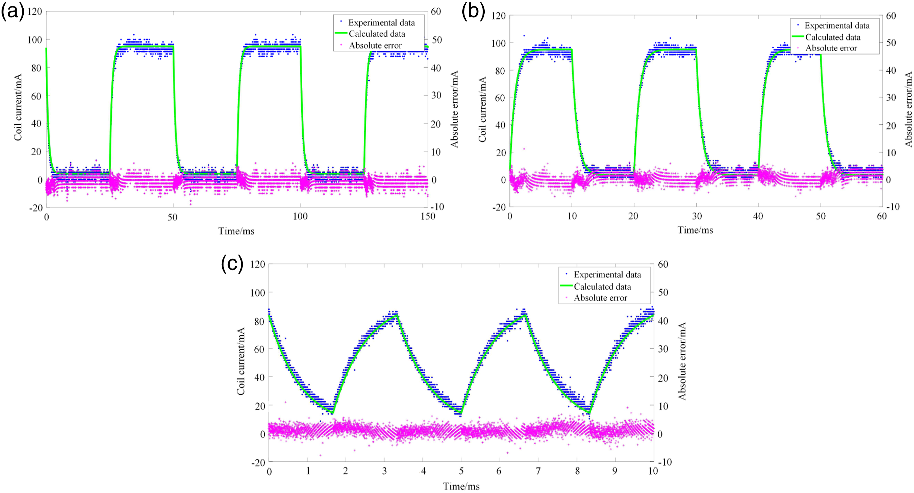

Validation of the multi-objective optimization

To validate the multi-objective optimization scheme in this paper, the responses of all coils are obtained and plotted in Figure 24. It can be discovered that the steady state intensity changes a lot with different wire diameters. However, in contrast, the response speed seems a bit hard to compare, for the difference looks not significant enough.

Figure 24.

Comparison of response under square wave excitation of Coil 1∼6.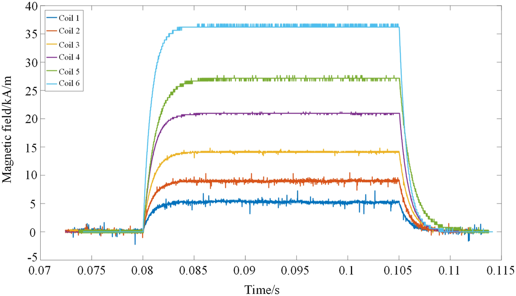

Aiming to analyze the results in a more clear way, the response time and the steady state current in each coil are extracted and compared with the calculation values, shown as Figure 25.

Figure 25.

Detailed response information of coil 1∼6. (a) Magnetic field intensity (b) Response time.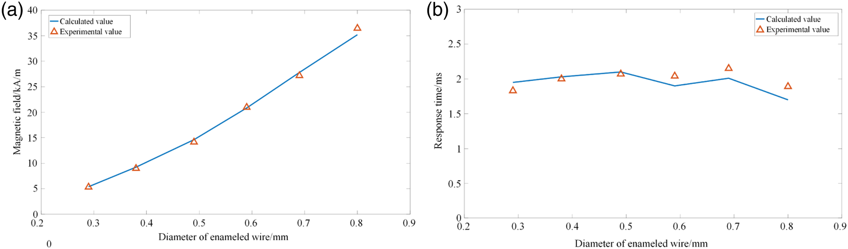

It can be seen from Figure 25 that the calculated results can well predict the actual results obtained from the experiments, with the maximum relative error about 3.45% in magnetic field intensity calculation, and 9.85% in response time calculation. While computing the response time, the error seems larger than that in magnetic field calculation, which should be explained by the reason that the testing noises make it hard to get the accurate response time from experimental results. In addition, from the results, it can be detected that the steady state magnetic field intensity goes up remarkably as the wire diameter increases. However, the changing trend of the response time is not very clear, for the inner and outer diameters of the enameled wire increase simultaneously. In addition, the best choice among the prototypes is Coil 6, with its dimensions very close to the optimal range.

Discussion

From the experimental results and the corresponding analysis, it can be concluded that the proposed method can well perform the multi-objective optimization for coil design of GMA. However, it cannot be neglected that there are a few problems still waiting to be solved in the next step, which are listed as follows:

(1) The optimization-oriented coil model needs to be further improved. Although the model results agree well with the experimental results in most cases, it can be discovered that some deviations exist, especially when the response current inside the coil is not too large. This phenomenon indicates that some improvements can be made on the coil model.

(2) Processing of the experimental data needs to be carefully investigated. In this paper, the experimental data have not been processed to suppress the noises before comparing with the model data, for the noises do not influence the data too much. However, as the noises indeed exist, the data processing methods like filtering should be added. And using this, it can be more easily to quantitatively compare the experimental data and the model ones.

Conclusions

This work provides a general roadmap targeting excitation coil modeling and optimization for GMA used in ECI. The theoretical analysis and experimentation work have set a foundation for further research on design and application of GMA. Several conclusions of this work can be drawn as follows:

(1) An optimization-oriented excitation coil model is established for GMA, in which the model parameters can be directly calculated by the coil dimensions.

(2) Utilizing the established model, the sinusoidal and square wave responses of the excitation coil are analyzed, which provides a concise method to predict the final coil performance under different excitation forms.

(3) The influence of coil dimensions on its response is investigated. Multi-objective optimization is conducted to balance the interaction between the response speed and the steady state magnetic field, and the optimal dimensional parameter range can be obtained.

(4) Using enameled wires in different parameters, several coil prototypes are manufactured. A series of experiments are completed, and the results indicate that the excitation coil model can well describe the current response throughout the operating frequencies, and the optimization scheme can serve as a good guideline to design excitation coil for GMA in high performance ECI.

Footnotes

Declaration of conflicting interests

The author(s) declared no potential conflicts of interest with respect to the research, authorship, and/or publication of this article.

Funding

The author(s) disclosed receipt of the following financial support for the research, authorship, and/or publication of this article: This work is supported by National Natural Science Foundation of China (Project No.51275525) and First Batch of Yin Ling Fund (Project No.ZL3H39).

Data availability

The data that support the findings of this study are available from the corresponding author upon reasonable request.

ORCID iD

Ce Rong

Calculation of equation ( 27 )

When the excitation coil experience voltage rising, the difference between the steady-state currents in the high voltage and low voltage can be expressed as (A.1)

Δ I = \frac{U_{h}}{R} - \frac{U_{l}}{R}

The time, when the current changing amplitude reaches 0.9ΔI, has been regarded as the characteristic parameter to evaluate the response speed of the coil. Therefore, the rising time of the coil current from U _l/R to (0.1U _l/R+0.9U _h/R) needs to be calculated. As the actual excitation waveform is displayed in Figure 7, the steady state coil current at the time point t ₁ is U _l/R. Combining equation (20) and (21), the coil current at the time point t ₂ can be calculated as the sum of the two branches as follows (A.2)

{\begin{cases} i_{r} (t_{2}) = i_{r 1} (t_{2}) + i_{r 2} (t_{2}) (a) \\ i_{r 1} (t_{2}) = (\frac{U_{l}}{R} - \frac{A t_{1}}{R} + \frac{A L}{R^{2}} - \frac{B}{R}) e^{- \frac{R}{L} (t_{2} - t_{1})} + \frac{A t_{2}}{R} - \frac{A L}{R^{2}} + \frac{B}{R} (b) \\ i_{r 2} (t_{2}) = C_{p} A (c) \end{cases}

In the high level voltage phase, as no current exists in the capacitor branch, the response time can be calculated by the expression of i _h(t) as (A.3)

i_{r 1} (t_{2}) = i_{h 1} (t_{2})

(A.4)

(\frac{U_{l}}{R} - \frac{A t_{1}}{R} + \frac{A L}{R^{2}} - \frac{B}{R}) e^{- \frac{R}{L} (t_{2} - t_{1})} + \frac{A t_{2}}{R} - \frac{A L}{R^{2}} + \frac{B}{R} = C_{2} e^{- \frac{R}{L} (t_{2} - t_{2})} + \frac{U_{h}}{R}

(A.5)

C_{2} = (\frac{U_{l}}{R} - \frac{A t_{1}}{R} + \frac{A L}{R^{2}} - \frac{B}{R}) e^{- \frac{R}{L} (t_{2} - t_{1})} + \frac{A t_{2}}{R} - \frac{A L}{R^{2}} + \frac{B}{R} - \frac{U_{h}}{R}

where C ₂ is a constant, and can be obtained by the continuity of the coil current at the time point t ₂ as follows (A.6)

i_{h} (t) = i_{h 1} (t) = C_{2} e^{- \frac{R}{L} (t - t_{2})} + \frac{U_{h}}{R}

Substituting (0.1U _l/R+0.9U _h/R) into equation (A.3), and the following expressions can be obtained (A.7)

C_{2} e^{- \frac{R}{L} (t - t_{2})} + \frac{U_{h}}{R} = \frac{0.1 U_{l}}{R} + \frac{0.9 U_{h}}{R}

(A.8)

t_{o n} = t - t_{2} = - \frac{L}{R} \ln [\frac{1}{C_{2}} (\frac{0.1 U_{l} - 0.1 U_{h}}{R})]

Substituting equation (A.5) into equation (A.8), the response time t _on can be expressed by (A.9)

t_{o n} = - \frac{L}{R} \ln \frac{(0.1 U_{l} - 0.1 U_{h})}{[(U_{l} - A t_{1} + \frac{A L}{R} - B) e^{- \frac{R}{L} (t_{2} - t_{1})} + A t_{2} - \frac{A L}{R} + B - U_{h}]}

Calculation of equation ( 30 )

Substitute equation (6), (7), and equation (8) into equation (27), the derivation process of L/R can be expressed as follows (B.1)

\begin{array}{l} \frac{L}{R} = \frac{\frac{μ_{0}}{4 π} N^{2} d_{s} Φ_{s} - \frac{π}{8} μ_{0}^{2} N^{2} \frac{d}{α^{2}} Γ (α, ρ, β)}{\frac{4 ρ_{r} k_{l} k_{N} a b (b + c)}{d_{h}^{2} d_{l}^{2}}} = \frac{\frac{μ_{0}}{4 π} {(\frac{k_{N} a b}{d_{h}^{2}})}^{2} d_{s} Φ_{s} - \frac{π}{8} μ_{0}^{2} {(\frac{k_{N} a b}{d_{h}^{2}})}^{2} \frac{d}{α^{2}} Γ (α, ρ, β)}{\frac{4 ρ_{r} k_{l} k_{N} a b (b + c)}{d_{h}^{2} d_{l}^{2}}} \\ = \frac{\frac{μ_{0} k_{N}^{2} a^{2} b^{2}}{4 π d_{h}^{2}} d_{s} Φ_{s} - \frac{π}{8} μ_{0}^{2} \frac{k_{N}^{2} a^{2} b^{2}}{d_{h}^{2}} \frac{d}{α^{2}} Γ (α, ρ, β)}{\frac{4 ρ_{r} k_{l} k_{N} a b (b + c)}{d_{l}^{2}}} = \frac{\frac{μ_{0} k_{N}^{2} a^{2} b^{2} d_{l}^{2}}{4 π d_{h}^{2}} d_{s} Φ_{s} - \frac{π}{8} μ_{0}^{2} \frac{k_{N}^{2} a^{2} b^{2} d_{l}^{2}}{d_{h}^{2}} \frac{d}{α^{2}} Γ (α, ρ, β)}{4 ρ_{r} k_{l} k_{N} a b (b + c)} \\ = \frac{\frac{μ_{0} k_{N}^{2} a^{2} b^{2} d_{l}^{2}}{4 π d_{h}^{2}} (b + c) Φ_{s} - \frac{π}{8} μ_{0}^{2} \frac{k_{N}^{2} a^{2} b^{2} d_{l}^{2}}{d_{h}^{2}} \frac{d}{α^{2}} Γ (α, ρ, β)}{4 ρ_{r} k_{l} k_{N} a b (b + c)} = \frac{μ_{0} k_{N} a b d_{l}^{2} Φ_{s}}{16 π d_{h}^{2} ρ_{r} k_{l}} - \frac{π μ_{0}^{2} d_{l}^{2} k_{N} a b Γ (α, ρ, β)}{32 d_{h}^{2} ρ_{r} k_{l} α^{2}} \\ = \frac{d_{l}^{2}}{d_{h}^{2}} (\frac{μ_{0} k_{N} a b Φ_{s}}{16 π ρ_{r} k_{l}} - \frac{π μ_{0}^{2} k_{N} a b Γ (α, ρ, β)}{32 ρ_{r} k_{l} α^{2}}) = \frac{d_{l}^{2}}{d_{h}^{2}} k_{N} a b (\frac{μ_{0} Φ_{s}}{16 π ρ_{r} k_{l}} - \frac{π μ_{0}^{2} Γ (α, ρ, β)}{32 ρ_{r} k_{l} α^{2}}) \end{array}

Therefore, equation (B.1) can be further simplified as (B.2)

{\begin{array}{l} \frac{L}{R} = \frac{d_{l}^{2} F (a, b, c)}{d_{h}^{2}} \\ F (a, b, c) = k_{N} a b (\frac{μ_{0} Φ_{s}}{16 π ρ_{r} k_{l}} - \frac{π μ_{0}^{2} Γ (α, ρ, β)}{32 ρ_{r} k_{l} α^{2}}) \end{array}

Then the response time t _on can be calculated as follows (B.3)

\begin{array}{l} t_{o n} = - \frac{L}{R} \ln \frac{(0.1 U_{l} - 0.1 U_{h})}{[(U_{l} - A t_{1} + \frac{A L}{R} - B) e^{- \frac{R}{L} (t_{2} - t_{1})} + A t_{2} - \frac{A L}{R} + B - U_{h}]} \\ = - \frac{d_{l}^{2} F (a, b, c)}{d_{h}^{2}} \ln \frac{(0.1 U_{l} - 0.1 U_{h})}{[(U_{l} - A t_{1} + A \frac{d_{l}^{2} F (a, b, c)}{d_{h}^{2}} - B) e^{- \frac{d_{h}^{2} (t_{2} - t_{1})}{d_{l}^{2} F (a, b, c)}} + A t_{2} - A \frac{d_{l}^{2} F (a, b, c)}{d_{h}^{2}} + B - U_{h}]} \\ = - \frac{d_{l}^{2} F (a, b, c)}{d_{h}^{2}} \ln \frac{(0.1 U_{l} - 0.1 U_{h}) d_{l}^{2}}{[(U_{l} d_{h}^{2} - A t_{1} d_{h}^{2} + A d_{l}^{2} F (a, b, c) - B d_{h}^{2}) e^{- \frac{d_{h}^{2} (t_{2} - t_{1})}{d_{l}^{2} F (a, b, c)}} + A t_{2} d_{h}^{2} - A d_{l}^{2} F (a, b, c) + B d_{h}^{2} - U_{h} d_{h}^{2}]} \end{array}

References

Xue

Zhang

, et al. A review of giant magnetostrictive injector (GMI). Sens and Actuators, A 2018; 273: 159–181.

Sun

Liu

Hu W

, et al. Design optimization of a giant magnetostrictive driving system for large stroke application considering vibration suppression in working process. Mech Syst Signal Process 2020; 138: 106560.

Wang

Zhang

, et al. A highly temperature-stable and complete-resonance rotary giant magnetostrictive ultrasonic system. Int J Mech Sci 2022; 214: 106927.

Zhou

Shi

, et al. Design and experimental perforamce of an inertial giant magnetostrictive linear actuator. Sens and Actuators, A 2020; 301: 111771.

Liu

Zhao

Wang

, et al. Study on model and characteristics analysis of the magnetostrictive drive component of automotive fuel injection system. Chin J Sen Actuators 2016; 29: 1797–1803.

Xue

Zhang

, et al. Design and model for the giant magnetostrictive actuator used on an electronic controlled injector. Smart Mater Struct 2017; 26: 05LT02.

Xue

Zhang

, et al. Equivalent circuit and driving voltage suitable for giant magnetostrictive actuator in electric injector. Electr Mach Contr 2016; 20: 20–28.

Gao

Liu

Guo

, et al. Structural design of giant magnetostrictive actuator. AIP Adv 2018; 8: 065211.

Huang

. Optimization of 3D magnetic field of double coil giant magnetostrictive transducer. J Mech Electr Eng 2019; 36: 544–548.

10.

Yang

Zhu

. Charateristic investigations on magnetic field and fluid field of a giant magnetostrictive material-based electro-hydrostatic actuator. Proc Imeche G: J Aerospace Eng 2017; 232: 847–860.

11.

Gao

Liu

Pei

, et al. Optimization and design of exiting coil in giant magnetostrictive actuator. In: 8th International Conference on Intelligent Robotics and Applications (ICIRA), Portsmouth, UK, 24-27 August 2015, pp. 190–200.

12.

Yang

Zhu

Fei

. Magnetic field analysis and optimization of giant magnetostrictive electro-hydrostatic actuator. J Aerospace Power 2016; 31(9): 2210–2217.

13.

Fan

Feng

Ying

. Optimum design of transmission coil for giant magnetostrictive actuator. In: International Conference on Optielectronic Science and Materials (ICOSM), Hefei, China, 20–22 September 2019. p. 012057.

14.

Bai

Zhang

Wang

, et al. Numerical evalutation and experimental test on a new giant magnetostrictive transducer with low heat loss design. Micromachines 2021; 12(11): 1397.

15.

Zhong

Wang

, et al. Magnetic field optimal analysis and experimental verification of giant magnetostrictive driving micro pump. Sci Technol Eng 2017; 17: 208–212.

16.

Fan

. Design and Research on a Cylindrical Giant Magnetostrictive Actuator. Master Thesis. China: Shandong University, 2017.

17.

Xue

Zhang

, et al. Displacement model and driving voltage optimization for a giant magnetostrictive actuator used on a high-pressure common-rail injector. Mater Des 2016; 95: 501–509.

18.

Chowdhury

Olabi

. Implementation of magnetostrictive material Terfenol-D in CNG fuel injection actuation. Adv Mater Res 2008; 47–50: 916–919.

19.

Ghodsi

Hosseinzadeh

Ozer

, et al. Development of gasoline direct injector using giant magnetostrictive materials. IEEE Trans Magn 2017; 53: 521–529.

20.

Xue

, et al. Magnetic field intensity model for giant magnetostrictive rod and coil optimization analysis. Nanotechnol Precis Eng 2014; 12: 85–90.

21.

Xie

Wang

, et al. Design of large-stroke and high resolution drive system based on giant magnetostrictive material. Int J Precis Eng Manuf 2021; 22: 799–811.

22.

Wang

Han

, et al. A model of giant magnetostrictive actuator used in automobile engine fuel injection system. Int J Serv Comp Orien Manuf 2013; 1: 154–166.

23.

Rong

, et al. Dynamic modeling and analysis of stack giant magnetostrictive actuator. Sens and Actuators, A 2018; 276: 205–218.

24.

Zhou

Zhang

Feng

, et al. An amplitude prediction model for a giant magnetostrictive ultrasonic transducer. Ultrasonics 2020; 108: 106017.

25.

Karasu

Altan

Bekiros

, et al. A new forecasting model with wrapper-based feature selection approach using multi-objective optimization technique for chaotic crude oil time series. Energy 2020; 212: 118750.

26.

Altan

Karasu

Zio

. AA new hybrid model for wind speed forecasting combining long short-term memory neural network, decomposition methods and grey wolf optimizer. Appl Soft Comput 2021; 100: 106996.

27.

Rong

Zhou

, et al. Model predictive sliding mode control for stack giant magnetostrictive actuators. Opt Precis Eng 2018; 26: 1680–1690.

28.

Zhou

Bai

, et al. Angular displacement modeling and excitation signal optimization for a stepping giant magnetostrictive rotary actuator. Rev Sci Instrum 2019; 90: 125002.

29.

Zhang

, et al. Research and experimental analysis on equivalent circuit models for giant magnetostrictive actuators. Proc CSEE 2018; 38: 3375–3383.

30.

Chen

Liu

Luo

, et al. Handbook of Inductance Calculations. Beijing: China Machine Press, 1992.

Physics-based modeling and multi-objective parameter optimization of excitation coil for giant magnetostrictive actuator used on fuel injector

Abstract

Keywords

Introduction

Structure of GMA for the fuel injector

Physics-based model of the excitation coil

Model of the excitation coil dimensions

Model of the excitation coil circuit

Response analysis of the coil circuit model

Response of the sinusoidal excitation

Response of the square excitation

Parameter optimization of the excitation coil

Analysis of the magnetic field intensity

Analysis of the response time

Parameter optimization of the excitation coil

Experimentation and model validation

Validation of the coil model

Validation of the coil circuit model

Validation of the response current model

Validation of the multi-objective optimization

Discussion

Conclusions

Footnotes

Declaration of conflicting interests

Funding

Data availability

ORCID iD

Calculation of equation ( 27 )

Calculation of equation ( 30 )

References