Sage Journals: Discover world-class research

Abstract

Aiming at researching on health monitoring of composite materials, a static load position identification method for optical-fiber composite structures based on the Particle Swarm Optimization-Back Propagation (PSO-BP) neural network algorithm is proposed. Based on the 2 × 2 optical fibers-composite structures, the PSO-BP algorithm is used to establish a nonlinear mapping between the fiber output intensity and the position. At first, a three-layer BP neural network is established. The number of the hidden layer is 30. And then the PSO algorithm is used to optimize the initial weights and thresholds of the BP neural network. Finally, a BP neural network is built using optimized initial weights and thresholds. A total of 515 sets of data samples are collected by the experimental system, of which 500 sets are used for training and 15 sets are used for the final model prediction. Simulation results show that the Mean Square Error (MSE) of the static load position prediction based on the PSO-BP algorithm is 0.0485. Compared with the position prediction model established by the BP neural network, Radial Basis Function (RBF) neural network and Support Vector Regression Machine (SVRM), the PSO-BP neural network model has a higher accuracy. The proposed method has an important application value for the research of health self-diagnosis of composite structures.

Keywords

Static load position prediction PSO-BP optical fiber-composite structures

Introduction

Due to its small size, light weight, anti-corrosion, and anti-electromagnetic interference, optical fiber has good sensing performance. It is very suitable for composites health monitoring. Moreover, optical fiber has strong plasticity, which is suitable for various shapes of composite components, and is widely used in the field of aerospace.^1,2 There are many kinds of fiber optic sensors³ used in composite structure health monitoring, including Bragg grating fiber optic sensors, Fabry Perot-Paro (F-P) optical fiber sensor, distributed optical fiber sensors, micro bend fiber optic sensor, etc. At present, various optical fibers have been widely used in the health monitoring of composite material structures, and there are many research results. Montoya et al.⁴ used 20 Fiber Bragg Gratings (FBGs) embedded into the composite front spar of the aircraft’s wing to collect the optical signals during flight. Through the comparison of the original structure signal and the damaged structure signal, the damage degree of the wing can be judged. The performance of the damage detection demonstrated a highest accuracy of 0.981. It realized the real time strain monitoring, remote sensing, and damage self-diagnosis of aircraft structure in service. Shan et al.⁵ established a method of strain monitoring on composite structures and strategy of damage identification based on distributed optical fiber sensors. It can basically realize the millimeter level accuracy identification and positioning of optical fiber distribution area. The monitoring error is about 4 mm. However, in Montoya et al.⁴ and Shan et al.,⁵ there were not any related algorithm used to process collected signals.

Generally, the information obtained by fiber optic sensor cannot directly get the health status including loading or damage positions information of composite structures. It is necessary to use some methods to process the fiber optic sensor information to complete the damage or load position identification of composite structures. Artificial Neural Network (ANN) is one of common models used for data regression or classification. With the development of mathematics and technology, many ANNs have been proposed, such as Feedforward Neural Network (FNN), Convolutional Neural Network (CNN), Recurrent Neural Network (RNN), etc.

FNN is the earliest artificial neural network invented and it is simple. It consists of multiple Logistic regression models (Continuous nonlinear function). It has an excellent non-linear mapping ability. CNN is a deep FNN with local connections and weight sharing. It is mainly used in various tasks of image and video analysis, and its accuracy is generally far beyond other neural network models. RNN is a kind of neural network with short-term memory ability. Compared with FNN, RNN is more consistent with the structure of biological neural network. It has been widely used in speech recognition, speech model and natural language generation.

Kharwar PK et al.⁶ platformed on the modeling of surface roughness during milling of Multiwall Carbon Nanotube (MWCNT) reinforced polymer nanocomposites using ANN. The Feed Forward BP network was used for the ANN model with TRAINLM and LEARNGDM functions used as training and learning algorithms. The designated model had high accuracy with correlation coefficient (R²) > 99%, MSE < 0.2%, and the average percentage error (APE) < 3%. In Altan et al.,⁷ neural network based real-time control of a hexarotor Unmanned Aerial Vehicle (UAV) was performed so that the payloads on the targets determined by path tracking could be left with minimum error. The Nonlinear Auto Regressive Xogenous (NARX) model of the UAV was obtained after the flight data were passed through the preprocessing, feature extraction and feature selection stages. It was tested that the performance of the model-based controller realized with the proposed NARX neural network model is very good and robust according to the Proportion Integral Differential (PID) controller. Califano et al.⁸ presented an implementation of a method for the structural health monitoring of composite structures supported by ANN. In contrast with other machine-learning-based Structure Health Monitoring (SHM) techniques, the presented ANNs-based approach did not need to be supported by data reduction procedures and, as the algorithm was trained using only “positive” (i.e. healthy) samples, it did not need to be associated to damage patterns. The proposed method is less time-consuming and less computational-expensive. Wang et al.⁹ proposed a quantitative monitoring method of delamination damage based on neural network to monitor the delamination damage area of composite structures accurately and quantitatively. The results showed that the proposed method can quantity monitoring the delamination damage of composites panel accurately, and the error of damage area is below 25%. Li et al.¹⁰ used the intelligent composite material impact location recognition technology based on the BP neural network system to obtain the time-domain signal response value of the FBG sensor to predict the impact position of the composite material. Simulation results showed that the BP neural network algorithm has the advantages of strong nonlinear approximation ability, high fault tolerance, and strong adaptive ability. It can realize the parameterized identification and positioning of composite laminates, and the ratio of the prediction results to the total length of the composite laminates to be tested less than 0.1.

From references 6 to10, only one type of ANN algorithm was used to make prediction. In Kharwar and Verma⁶ and Li et al.,¹⁰ methods used were Feed Forward BP network. If it can be used in combination with other optimization algorithms, the prediction accuracy may be improved.

Although ANNs have many advantages, such as BP neural network. It has a good nonlinear mapping ability, self-learning and adaptive ability, generalization ability, and fault-tolerant ability. But it also has great limitations, such as easy local convergence, slow convergence speed, strong sample dependence, and easy over fitting.¹¹ To overcome these shortcomings, some optimization algorithms are usually used to optimize the parameters of neural network, such as Genetic Algorithm (GA), Particle Swarm Optimization (PSO), Ant Colony Optimization (ACO), Grey Wolf Optimizer (GWO), and so on.^12–16

At present, the use of hybrid algorithms has become the choice of more scholars, such as Grey Wolf Optimizer-Long Short-Term Memory (GWO-LSTM), Multi-Objective-Particle Swarm Optimization-Grey Relation Analysis (MOPSO-GRA), Multi-Objective-Particle Swarm Optimization-Radial Basis Function based Support Vector Regression (MOPSO-RBFSVR), GA-ANN, Continuous Genetic Algorithm- Particle Swarm Optimization (CGA-PSO), etc.

Altan et al.¹² developed a new hybrid wind speed forecasting (WSF) model based on LSTM network and decomposition methods with GWO. The obtained experimental results indicated that the proposed combined model can capture non-linear characteristics of wind speed time series (WSTS), achieving better forecasting performance than single forecasting models, in terms of accuracy. Kesarwani et al.¹³ highlighted the drilling experimentation of zero-dimensional (0-D) Carbon nano onion (CNO) reinforced polymer composite. The MOPSO is utilized to achieve optimal results from the multi-decision criterion for the Machining performance. Practical applications for the discovered relationships include using GRA to extract the most relevant finding from the Pareto Front space of optimal solutions. Using the GRA, the optimum solution was found. Karasu et al.¹⁴ developed a new forecasting model based on SVR. The features are selected by the wrapper-based approach consisting of MOPSO and RBFSVR techniques considering both the mean absolute percentage error (MAPE) and Theil’s U values. The obtained empirical results showed that better forecasting performance can be obtained in terms of precision and volatility than the other current forecasting models. Gomes et al.¹⁵ proposed an optimization procedure to minimize the maximum value of Tsai-Wu of laminated composite tubes subject to axial loading. ANNs and GAs are chosen as optimization tools. The results showed that the developed algorithm converges faster. Vosoughi ¹⁶ presented A new hybrid method for damage detection of laminated composite beams. In the method, a continuous genetic algorithm is improved by sensitivity modal analysis and PSO techniques. The added PSO and the sensitivity analysis operators improve the generated population before and after CGA, respectively in conjunction with an embedded micro search operation in genetic algorithm to reduce the search space. Applicability, efficiency, and robustness of the proposed algorithm in detecting the location and extent of damages in presence and absence of the PSO method for different examples are demonstrated.

Through the analysis of the above recent references, it can be known that the models established using the hybrid algorithm have excellent prediction results. Montoya et al.⁴ and Li et al.¹⁰ used are FBGs, and Shan et al.⁵ used are distributed optical fiber sensors to study on the health monitoring of composite structure. The difference is that this article studied the load position identification of 2 × 2 optical fiber-composite structures made of fiber sensors based on intensity modulation. Li et al.¹⁰ only used the BP neural network to predict the impact load position. The prediction accuracy can be improved if the algorithm is improved or optimized.

Due to the simpleness of the optical fiber – composite structures studied in this paper and the low dimension of data to be processed, the simplest FNN is considered to establish the load location model, and the BP neural network is one of the FNNs commonly used. And combined with the PSO algorithm to establish a PSO-BP neural network model, to achieve high-precision load position identification of composite structures. The essential principle of PSO is to use the current position, global extreme value, and individual extreme value to guide positions of next iteration particles. The key to PSO’s excellent characteristics is that individuals make full use of their own experience and group experience to adjust their own state. PSO algorithm is simple and easy to operate. It can remember the personal and global optimal information without crossover and mutation operation, and it has a high speed of approaching the optimal solution. It is easy to be combined with other intelligent algorithms to build many hybrid models.^14,16

So, aiming at the health monitoring of composites, this article proposes a static load position recognition method of optical fiber-composite structures based on PSO-BP algorithm. The mathematical model of load information and position information is established by using PSO-BP algorithm. Research results show that, compared with other algorithms, PSO-BP algorithm has higher accuracy in load position prediction. It has an important application value for the health self-diagnosis research of composite structures.

Experimental details

The experimental system is composed of light source, sensing fiber optic-composite structures, photoelectric detection module, Signal acquisition and processing module, and monitoring center. The experimental system structure diagram is shown in Figure 1.

Figure 1.

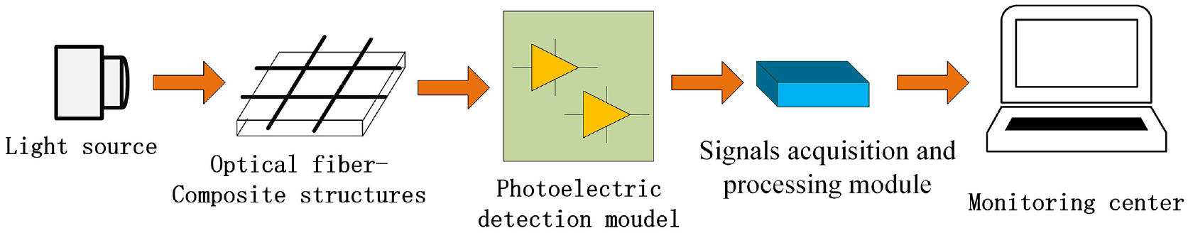
Experimental system structure diagram.

In Figure 1, the light source of the system is a laser, and the emission wavelength is 632.5 nm. The optical fiber-composite structure is constructed by orthogonally embedding 2 × 2 optical fibers into the composite materials.¹⁷ In this article, the glass fiber reinforced E-51 epoxy resin-based layered composite material is selected as the research object. Because it has a wide range of applications and is a prime candidate for buried sensor systems. In addition, the laminated structure of the composite material can also ensure the flexibility of design and construction, since these materials are composed of many layers. Optical fibers can be adjusted in the specified direction, which can meet the requirements of hardness and strength. The optical fiber used is an intensity-sensitive optical fiber sensor. In order to improve the sensitivity of the fiber during loading, the fiber is buried in the shallow layer of the composite material structure. The fabrication of the optical fiber-composite structure is completed in the laboratory. In order to ensure that fibers are not damaged during the production process, no more treatment on the surface of the composite. The actual product is shown in Figure 2(a). The area of the optical fiber-composite structure in the experimental system is 3 × 3 cm², and the distance between two parallel fibers is 1cm. As shown in Figure 2(b), Fi (i = 1, 2, 3, 4) is the number of fibers. Fibers as sensing elements are embedded in the composite board. When an external force acts on the surface of optical fiber-composite structure, the light intensity transmitted will change due to the deformation of embedded fibers. Thus, the optical signals transmitted in optical fibers will carry the load position information of the composite structure.

Figure 2.

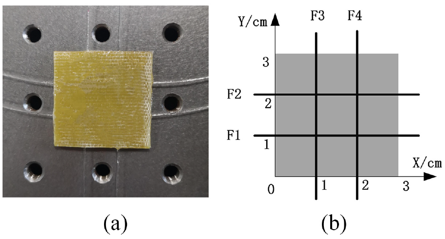
optical fiber-composite structure: (a) the actual experimental structure and (b) structure coordinate.

The photoelectric detection module is mainly responsible for optical signal reception, photoelectric conversion, and amplification. The module consists of a photoelectric converter, a photoelectric conversion circuit and the signal amplification circuit. The photoelectric converter is a Positive Intrinsic-Negative (PIN) avalanche photodiode. The signal amplifier circuit uses a T-type feedback network, and the core components are high-precision budget amplifiers OPA277 and LF353. The photoelectric detection module is shown in Figure 3. The power is ±5V.

Figure 3.

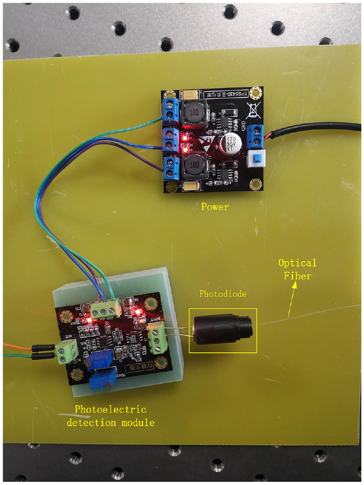
The photoelectric detection module.

The signal acquisition and processing module is composed of Digital Signal Processor (DSP). It is mainly responsible for receiving and processing the signal after photoelectric amplification and transmitting the data to the monitoring center. The monitoring center is a computer. It provides a visual monitoring interface to watch the change of signals and output light intensity value of fibers. The operating environment DSP software is Code Composer 4.1. The display interface is designed by C++ programming. Signals acquisition interface is shown in Figure 4. The display values of the text boxes F1, F2, F3, F4 are optical fiber outputs.

Figure 4.

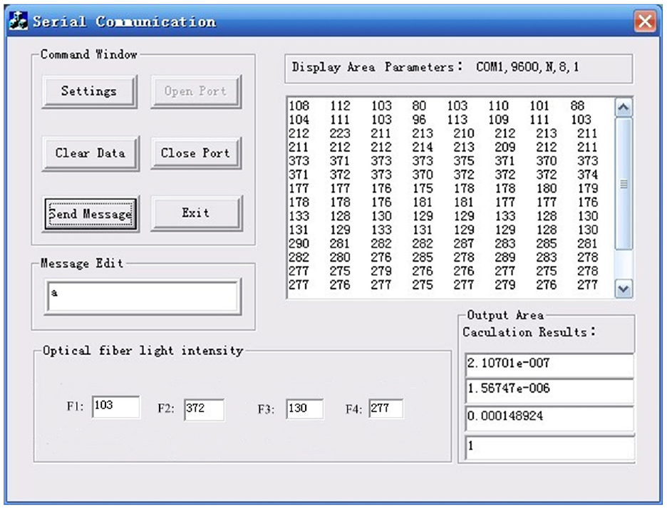
Signals acquisition interface.

Based on the above experimental system, load experiments are carried out on positions (X, Y) in the fiber-composite structure, and the fiber output values (F1, F2, F3, F4) are collected in the monitoring center. After a lot of experiments, a total of 515 sets of data sample [(F1, F2, F3, F4), (X, Y)] were collected. The design and simulation of load location algorithm based on PSO-BP neural network is implemented in MATLAB.

Methodology

BP neural network

The basic structure diagram of BP neural network¹⁸ is shown in Figure 5. It is generally composed of an input layer, a hidden layer, and an output layer. The input layer provides information through external input, and the nodes of each layer use the output of the previous layer as the input of the next layer. Neurons are the basic structural units of BP neural networks, which are distributed in each layer and connected to each other. When many neurons are connected in a certain way to form a neural network framework, a nonlinear mapping of input data and output data can be obtained.

Figure 5.

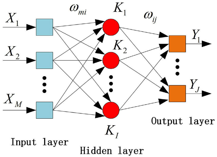
Basic structure diagram of BP.

The learning of BP neural network mainly includes two processes: the forward propagation process of input data and the back propagation process of error information. The input signal propagates along the direction of the input layer, hidden layer, and output layer. During the propagation process, the threshold and weight of the neural network remain unchanged. When the output result of the output layer is quite different from the training target, the neuron node of the output layer will produce error signal back propagation, thereby correcting the threshold and weight of the neural network. The two processes alternate until the error meets its output conditions. The specific learning process of BP neural network is as follows. As shown in Figure 5, M, I, and J are the number of neurons in the input layer, the number of neurons in the hidden layer, and the number of neurons in the output layer, respectively. X_m, K_i, Y_j are the input of the m-th neuron of the BP neural network, the output of the i-th neuron of the hidden layer, and the output of the j-th neuron of the output layer. ω_mi is the weight of the input layer, the input layer to the hidden layer. ω_ij is the weight of the hidden layer to the output layer. θ_i and θ_j are the threshold value of the j-th neuron in the hidden layer and the threshold value of the k-th neuron in the output layer. $f (•)$ and $g (•)$ are the activation functions of the hidden layer and the output layer. The function $f (•)$ can also be called “Transfer function,” The commonly used is the sigmoid function given as equation (1). The functions $g (•)$ use is a linear function.

f (x) = \frac{1}{1 + e^{- x}}

(1)

In the forward propagation of the signal, the output of the i-th neuron in the hidden layer is given as equation (2).

K_{i} = f (\sum_{m = 1}^{M} ω_{mi} X_{m} + θ_{i}) = f (ne t_{i})

(2)

net_i is the input of the i-th neuron in the hidden layer. The output function of the j-th neuron in the output layer is given as equation (3).

Y_{j} = g (\sum_{i = 1}^{I} w_{ij} X_{i} + θ_{j}) = g (ne t_{j})

(3)

net_j is the input of the j-th neuron in the output layer. Using R_j to represent the expected output of the j-th neuron in the output layer, the error between the actual output of the j-th neuron and the expected output is given as equation (4).

e_{j} = R_{j} - Y_{j}

(4)

The total error of the network output is given as equation (5).

E = \frac{1}{2} \sum_{j = 1}^{J} {(R_{j} - Y_{j})}^{2} = \frac{1}{2} \sum_{j = 1}^{J} {e_{j}}^{2}

(5)

If the total error of the output does not meet its end conditions, the weights and thresholds of the neural network are optimized through error back propagation. If they are met, the training ends.

In the back propagation process of the error signal, the gradient descent method is used to adjust the weight and threshold of the neuron, so that the error of the output layer meets the requirements. If z_i is the output error of the i-th neuron in the hidden layer, then

z_{i} = \sum_{j = 1}^{J} e_{j} \times θ_{j} \times f' (\sum_{m = 1}^{M} ω_{mi} x_{m} + θ_{i})

(6)

The threshold of the output layer is adjusted to equation (7).

θ_{j} (j + 1) = θ_{j} (j) + η \times e_{j}

(7)

The threshold of the hidden layer is adjusted to equation (8).

θ_{i} (j + 1) = θ_{j} (j) + η \times z_{i}

(8)

The connection weight between the hidden layer and the output layer is adjusted to equation (9).

w_{ij} (j + 1) = w_{ij} (k) + η \times e_{j} \times Y_{m}

(9)

The connection weight between the input layer and the hidden layer is adjusted to equation (10).

w_{mi} (j + 1) = w_{ij} (k) + η \times z_{i} \times X_{m}

(10)

Among them, η is the learning rate of the neural network.

PSO algorithm

PSO algorithm is a group optimization algorithm derived from the foraging behavior of bird groups.¹⁹ It mainly guides the optimization search through cooperation between bird groups and mutual search. In the PSO algorithm, the solution set of the optimization problem is abstracted into searching for particles in space. These particles have their own initial speed and position. The particles have their own optimal fitness value (pbest) and the current population of the entire population. Optimal fitness value (gbest) to adjust its position and speed. Iteratively search in the search space, and finally find the global optimal solution. The update formula of particle velocity and position is given as equations (11) and (12).

\begin{matrix} v_{n, d}^{k + 1} = w \times v_{n, d}^{k} + c_{1} \cdot r_{1} \cdot ({pbest}_{n, d}^{k} - x_{n, d}^{k}) \\ + c_{2} \cdot r_{2} \cdot ({gbest}_{n, d}^{k} - x_{n, d}^{k}) \end{matrix}

(11)

x_{n, d}^{k + 1} = x_{n, d}^{k} + v_{n, d}^{k + 1}

(12)

Where, $w$ is the inertia weight. $v_{n, d}^{k}$ and $x_{n, d}^{k}$ are the velocity and position of the d-th dimension of the particle n in the k-th generation. $c_{1}$ and $c_{2}$ are individual learning factors and social learning factors. $r_{1}$ and $r_{2}$ are random numbers between 0 and 1. ${pbest}_{n, d}^{k}$ and ${gbest}_{n, d}^{k}$ are the individual extremum and the global extremum of the d-th dimension of particle n in the k-th generation.

Establishment of PSO-BP neural network model

The establishment of the PSO-BP neural network load location model mainly includes three parts: Data set division and normalization, Parameter settings of BP neural network and parameter settings of PSO algorithm.

Data sets division and normalization

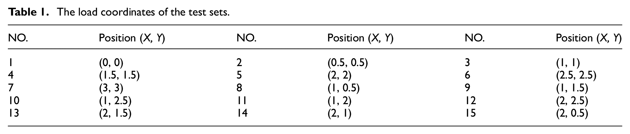
515 sets of data samples [F1, F2, F3, F4, X, Y] were collected. We try to load at various positions to ensure that the data samples are representative and balanced. Among the 515 sets of samples, 15 sets are used for the final test of the network model, and 500 groups are used to build the PSO-BP neural network model. Table 1 shows the load position coordinates of the 15 groups of test samples. It can be known that positions of the selected 15 groups of test samples are representative, from the edge position (0, 0), (3, 3) to the center position (2.5, 2.5) of the composite material.

Table 1.

The load coordinates of the test sets.

NO.	Position (X, Y)	NO.	Position (X, Y)	NO.	Position (X, Y)
1	(0, 0)	2	(0.5, 0.5)	3	(1, 1)
4	(1.5, 1.5)	5	(2, 2)	6	(2.5, 2.5)
7	(3, 3)	8	(1, 0.5)	9	(1, 1.5)
10	(1, 2.5)	11	(1, 2)	12	(2, 2.5)
13	(2, 1.5)	14	(2, 1)	15	(2, 0.5)

In the process of establishing the BP neural network model, a cross-validation method is adopted. Therefore, the 500 sets of data samples will be divided into training set, validation set and test set. The ratio is 400:50:50. But each set is randomly generated.

Due to the different sizes of the input data range, the input with a large data range has a larger effect on model, while the input with a small data range has a smaller effect. The activation function value range of the neural network output layer is limited, so it is necessary to map the target data of the network training to the range of the activation function. Based on the above analysis, all data sets need to be normalized. This article maps all data sets to the interval [0, 1]. Data sets are normalization using the following equation (13).

y = \frac{x - \min}{\max - \min}

(13)

The program code is as follows.

[inputn, inputps] = mapminmax (input_train);

[outputn, outputps] = mapminmax (output_train);

inputn_test=mapminmax (‘apply’, input_test, inputps);

an = sim (net, inputn_test);

test_simu = mapminmax (‘reverse’, an, outputps);

In order to calculate the test error, the PSO-BP network model test results are de-normalized.

Parameter settings of BP neural network

In this article, a three-layer BP neural network is established, which includes a hidden layer. [F1, F2, F3, F4] is the input of the neural network, [X, Y] is the output of the neural network. It can be known from Section 3.1 that there are several important parameters in BP algorithm. They are the number of hidden layers, learning rate, activation function, weight, and threshold. The number of hidden layers, learning rate, and activation function are set by ourselves and they are shown in Table 2.

Table 2.

Parameters of BP neural network.

Network type	BP
Transfer function	Hidden layer – Sigmoid Output layer – Linear
Training Algorithm	TRAINLM
Data division	Training data – 70% Validation data – 15% Test data – 15%
Hiddennum	30
net.trainParam.epochs	100
net.trainParam.lr	0.001
net.trainParam.goal	0.01

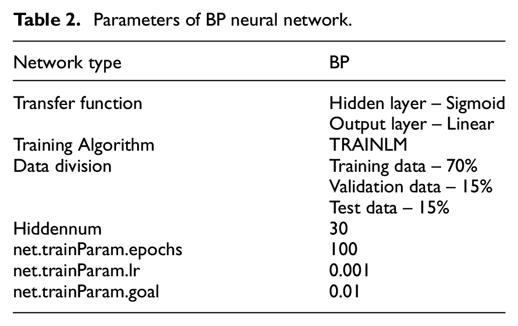
The activation function used is the “sigmoid” function shown in equation (1). The weight and threshold is usually initialized randomly.

The code for BP neural network is as follows.

net=newff (inputn, outputn, hiddennum); % Build the network

[net, tr]=train (net, inputn, outputn); %Training the network

an=sim (net, inputn_test); %Network prediction

The load position identification of composite material researched in this article is a complex problem with high-order nonlinear characteristics.²⁰ Random initialization of weights and thresholds usually causes the BP neural network to fall into local extreme points, which affects its nonlinear fitting ability and operating efficiency. It will also cause the instability of the BP neural network model. Therefore, the PSO algorithm is used to optimize the initial weights and thresholds of the BP algorithm.

Parameter settings of PSO algorithm

Although PSO is an optimization algorithm, it also has its parameters including fitness function, inertial weight $w$ , individual learning factor $c_{1}$ and social learning factor $c_{2}$ , number of iterations, velocity, population, and population size. The settings of these parameters will affect the performance of the established model. Random initialization of weights and thresholds usually causes the BP neural network to fall into local extreme points, which affects its nonlinear fitting ability and operating efficiency. Some PSO algorithm parameter settings are shown in Table 3.

Table 3.

Parameters of PSO algorithm.

Algorithm	PSO
Population size	20
Max iterations	80
$c_{1}$ , $c_{2}$	1.49445
inertial weight $w$	0.4 to 0.8
velocity	−0.5 to 0.5
Population	−3 to 3

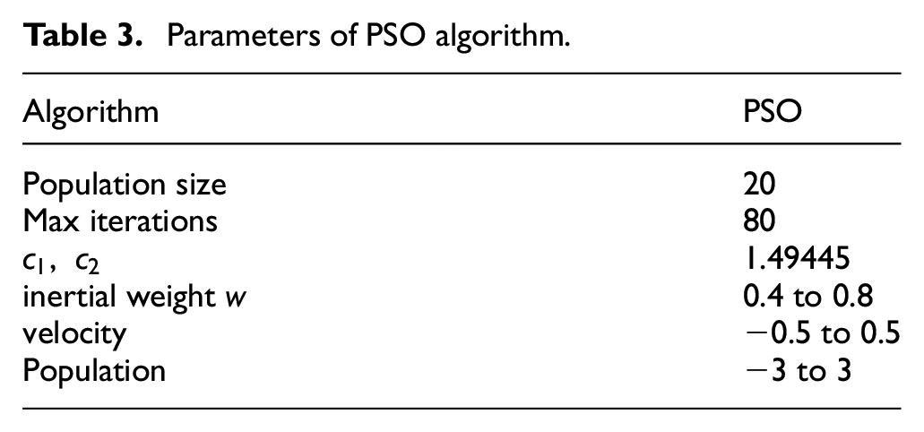
The population size is 20. Although the larger the initial population, the convergence will be better, but too large will also affect the velocity. Too few iterations, the solution is unstable, and too many iterations will cause long calculation time. For complex problems, evolutionary algebra can be improved accordingly. Here the number of iterations is set to 80. $c_{1}$ and $c_{2}$ are usually set to 1.49445. It is also necessary to set a reasonable velocity range. If the particle moving velocity is too fast, it is possible to cross the optimal solution. If the moving velocity is too slow, the convergence will be slow. Population is the search space, and it is limited to the interval [−3, 3].

The inertial weight $w$ is an important parameter, which determines the global search and local search of the PSO algorithm. When $w$ is larger, the value of $w \times v_{n, d}^{k}$ in equation (11) is larger, and global search will be performed. Otherwise, local search will be performed. In order to achieve global search and local search at the same time, $ω$ is set to the interval of 0.4–0.8, and the value is linearly changed. The expression of $ω$ is equation (14).

w = w_{\max} - (w_{\max} - w_{\min}) * j / maxiterations

(14)

Where j is the loop integer variable, $w_{\max} = 0.8, w_{\min} = 0.4, maxiterations = 80$ .

The fitness function used is the test error of the BP neural network. The program code of fitness function is as follows.

fitness (i, :)=fun(pop(i,:),inputnum, hiddennum, outputnum, net, inputn, outputn);

function err = fun (x, inputnum, hiddennum, outputnum, net, inputn, outputn)

err=0.5*sum (abs (ann- outputn));

where ‘ann’ is the training output of the network and ‘outputn’ is the desired output.

The prediction error is described by the Mean Square Error (MSE). The expression is given as Eq. (15)

MSE = \frac{1}{n} \sum_{i = 1}^{n} {(y_{i} - {y'}_{i})}^{2}

(15)

where $y_{i}$ is the desired Neural Network output, and ${y_{i}}^{'}$ is the test output of network.

In this article, the PSO algorithm is used to optimize the initial weights and thresholds of BP neural network. Weights and thresholds of BP neural network are defined as the individual particles. Calculating the fitness of the particles, the individual and global optimal are determined until the maximum number of iterations. After the optimization is completed, the optimized weights and thresholds are substituted into the BP neural network as the initial weights and thresholds, and the network is trained to complete the establishment of the PSO-BP neural network model.²¹ Finally, 15 sets of test samples are tested to obtain the prediction error of load positioning. The conversion graph of the PSO-BP neural network load position prediction model is shown in the Figure 6.

Figure 6.

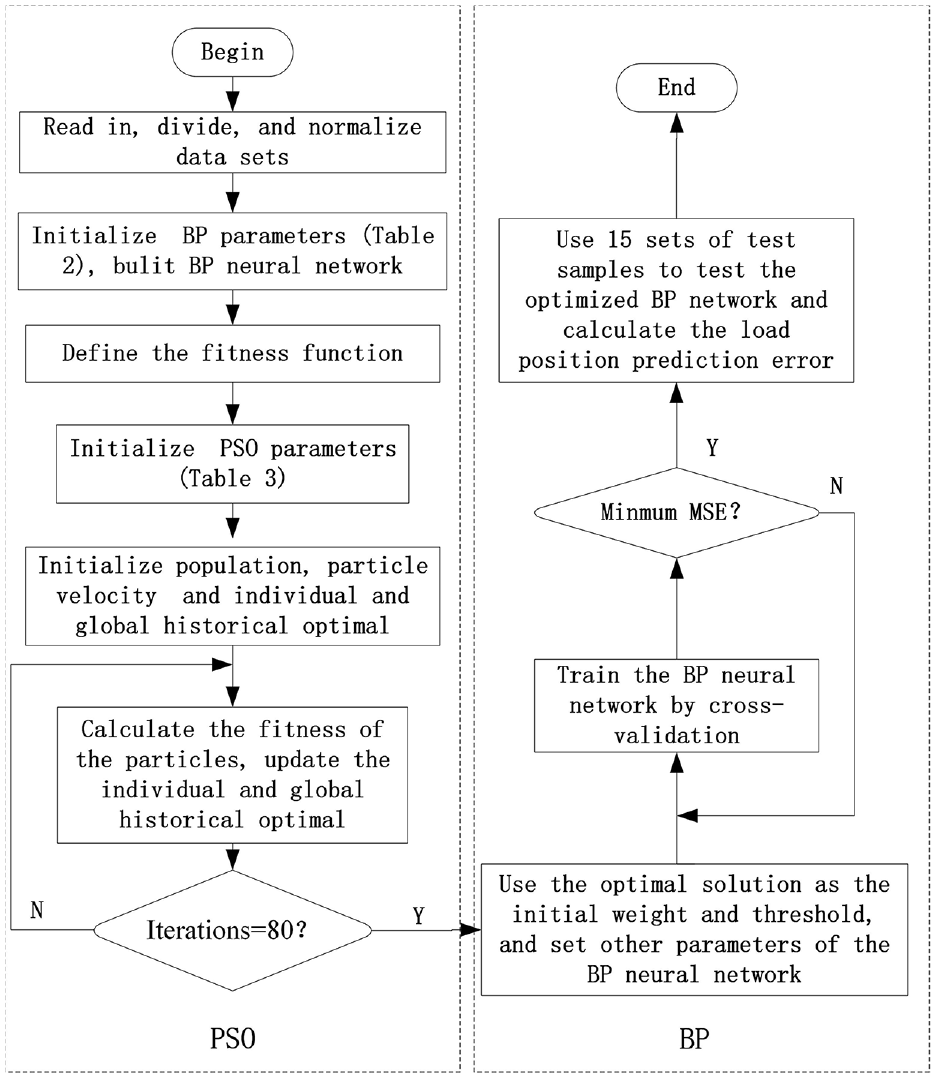
The conversion graph of PSO-BP neural network load position prediction model.

Results and discussion

BP and PSO-BP neural network prediction

Figure 5(a), (b), and (c) shows simulation results of the BP neural network model without optimization. As shown in Figure 7(a), the Regression values R of the training set, validation set, test set and overall for BP neural network model are 0.73758, 0.67461, 0.6903, and 0.7202, respectively. It can be known from Figure 7(b), the minimum error of the BP neural network during the training process is 0.56169. Figure 7(c) shows the prediction error of the load position (X, Y) of 15 sets of test samples, and the MSE of the test samples is 0.141684. The computation time of the BP neural network model is within 30 s.

Figure 7.

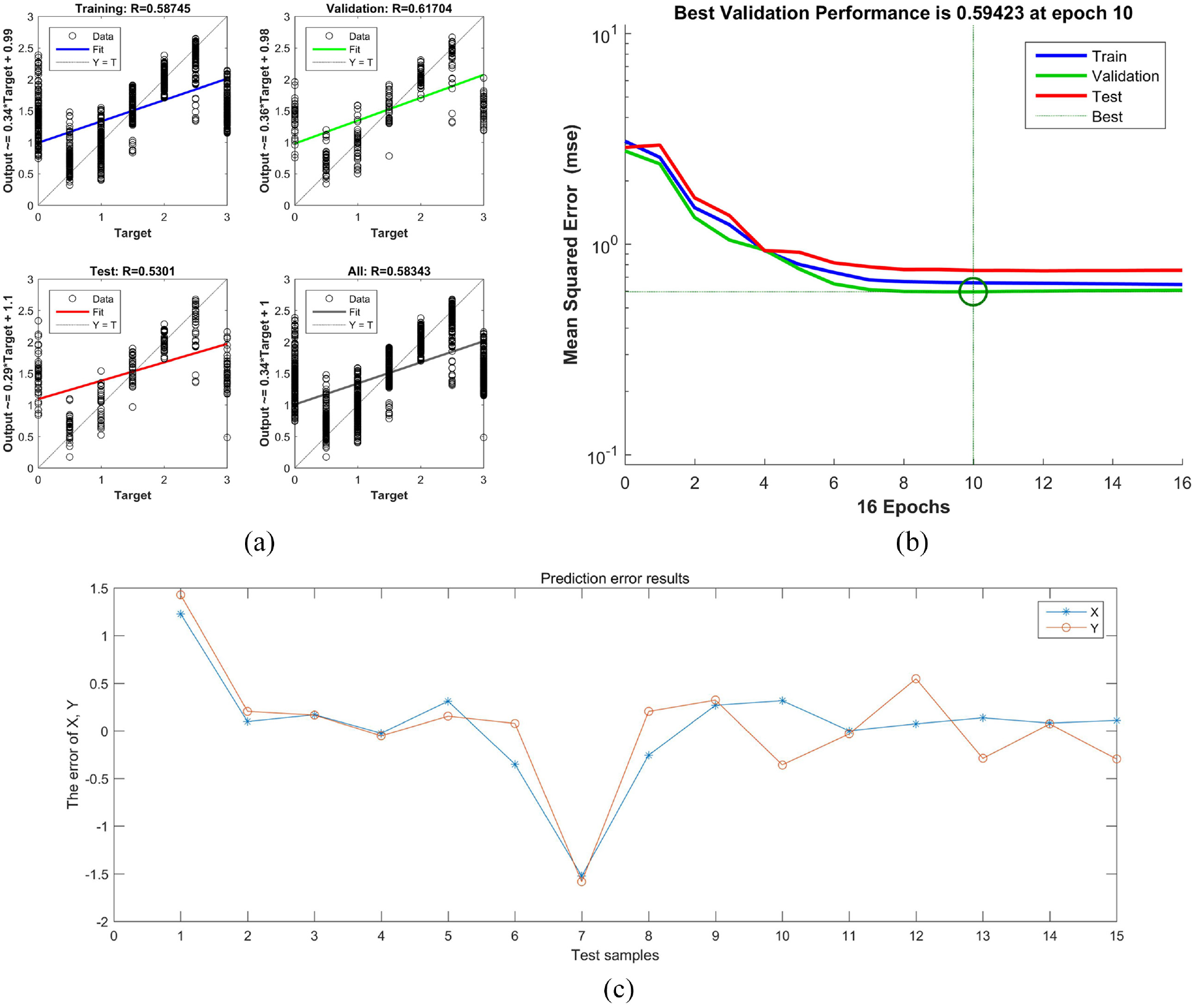
BP neural network model simulation results: (a) the correlation coefficient representation graph, (b) the training performance curve, and (c) the prediction error of coordinates (X, Y).

Simulation results of the BP neural network model optimized by the PSO algorithm are shown in Figure 8(a), (b), and (c). As shown in Figure 8(a), the R values of the training set, validation set, test set and overall for PSO-BP neural network model are 0.9708, 0.95219, 0.82511, and 0.94301, respectively. Figure 8(b) shows that the minimum error of the BP neural network during the training process is 0.04852. The prediction error of the load position (X, Y) is shown in Figure 8(c), and the mean square error (MSE) is 0.07515. And the computation time of the PSO-BP neural network model is about 15 min.

Figure 8.

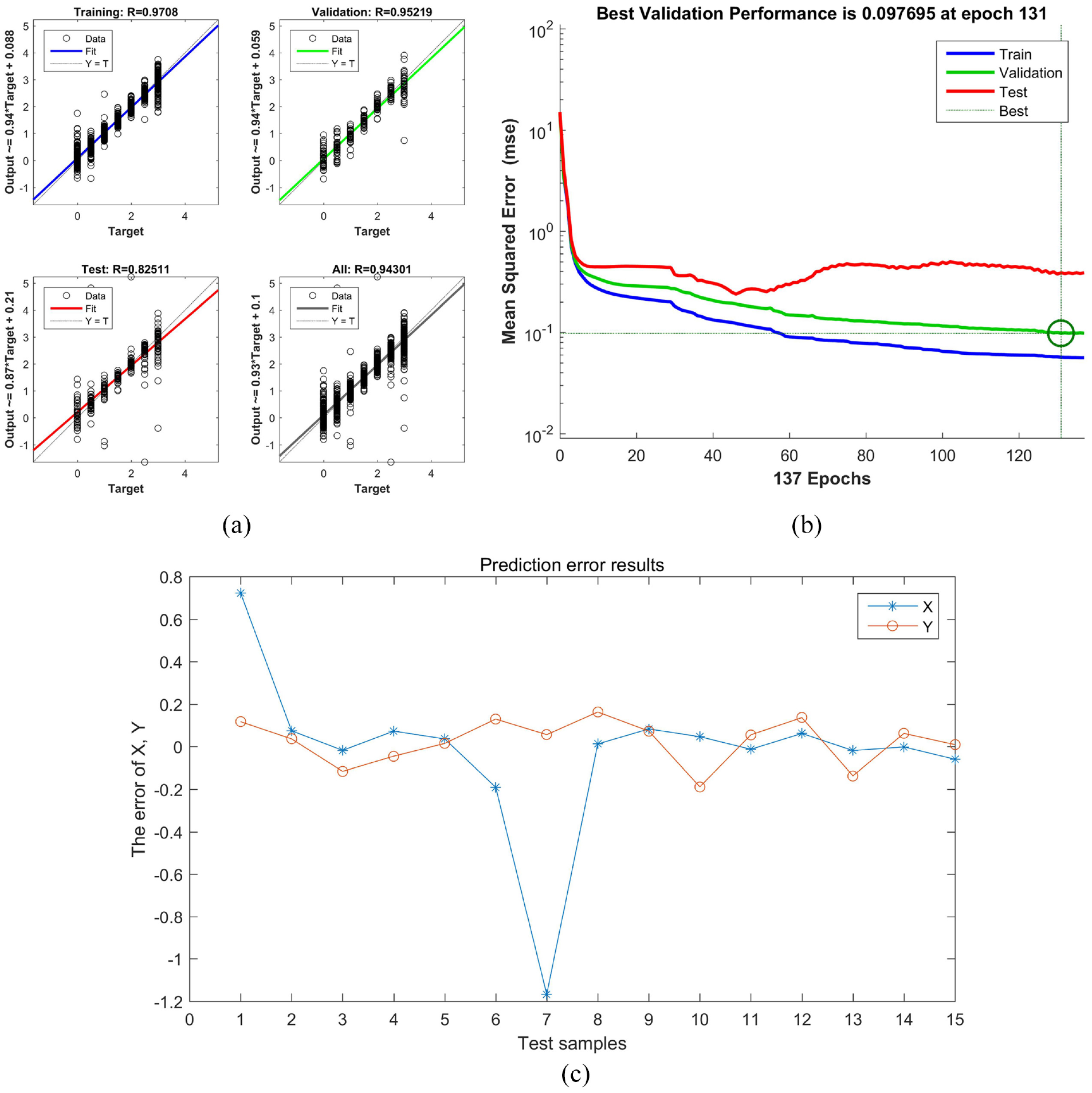
PSO- BP neural network model simulation results: (a) the correlation coefficient representation graph, (b) the training performance curve, and (c) the prediction error of coordinates (X, Y).

Figures 7 and 8 displays that the performance of PSO-BP network model is obviously better than that of BP neural network model. The prediction error of PSO-BP is higher, regardless of the R value, the best mean square error in the training process, or the MSE of the final test samples. In fact, it can be known that the R values of overall is 0.94 from Figure 8(a). And the R value of test is just 0.82. It is obvious not the best results. The reason for analysis is due to the imbalance and incompleteness of data samples. We tried our best to get 500 sets of data. But for a 3 cm × 3 cm composite board, there are infinite points can be loaded on. It is impossible to exhaust all points, only some representative positions can be used. Besides, there are only four fibers and four characteristic values in the experiment. It seems to be too little for higher precision position recognition.

It also can be known from Figures 7(c) and 8(c) that the prediction error of the first loading position (0, 0) and the seventh loading position (3, 3) are relatively large. The reason is that these two points belong to corner points of composite structures. When the load acts on these positions, there are no change in optical fibers outputs. It means that the characteristics of these positions are the same, so the network model will have a large error when predicting. Besides, the computation time of PSO-BP model is longer than BP model. The time is determined by the sample size, population size and number of iterations. Of course, it is also related to the performance of the computer.

Comparison with other algorithms

To verify the performance of the position prediction of PSO-BP neural network algorithm proposed in this article, the Radial Basis Function (RBF) neural network and Support Vector Regression Machine (SVRM) algorithm were used to identify the load position in the same data sets.

RBF neural network²² is an ANN that uses radial basis functions as activation functions. It is a linear combination of radial basis functions. This paper adopts a regularized RBF network structure, the number of hidden nodes is the number of samples, and the data center of the basis function is the sample itself, and only the expansion constant and the weight of the output node are considered. The expansion constant of the radial basis function can be determined according to the dispersion of the data center. In order to prevent each radial basis function from being too sharp or too flat, one option is to set the expansion constant of all radial basis functions to equation (16).

δ = \frac{d_{max}}{\sqrt{2 P}}

(16)

In the equation (16), $d_{max}$ is the maximum distance between samples; P is the number of samples. $δ$ is the parameter “spread” of RBF neural network.

Support Vector Machine is a kind of machine learning algorithm based on statistical theory. It is invented by Vapnik in 1995.²³ And now it is widely used in the fields of pattern recognition, classification, and Regression. There are three important model parameters in SVRM.²⁴ They are respectively penalty coefficient (c), the parameter (g) of RBF kernel function and the insensitive loss function ( $ε$ ). Among them, c is used to control the complexity and the approximation error of the model. The larger c, the higher the fitting degree of the training samples; g affects the complexity of the data samples distributed in high dimensional feature space; the value of $ε$ determines the number of the support vector.

This paper uses the grid search method to find the best values of parameters c and g. The value range of c, g is set in the interval [−10, 10], the search interval of parameter c is 0.2, and the search interval of g is 0.1. Create and train SVRM based on the searched “bestc” and “bestg.” The parameter $ε$ is set to 0.01. Some codes are as follows.

[c, g] = meshgrid (-10:0.2:10, -10:0.1:10); % Set the search range of c and g

%% search bestc and bestg

cmd = [‘-v’, num2str (v), ‘-t, 2’, ‘-c’, num2str (2 ^ c (i, j)), ‘-g’, num2str (2^g (i, j))];

cg(i, j) = svmtrain(inputn, outputn, cmd);

if cg(i, j)<error

error=cg(i,j);

bestc=2^c(i,j);

bestg=2^g(i,j);

%%%%

cmd = [‘-t 2’, ‘-c’, num2str (bestc), ‘-g’, num2str (bestg), ‘-s 3, -p 0.01’]; % Create SVR

model = svmtrain (inputn, outputn, cmd); % Train SVR

[predict, error] = svmpredict (inputest_test, output_test, model); % Predict

The MSE of different algorithms are shown in Table 4.

Table 4.

The MSE of different algorithms.

Algorithms	PSO-BP	BP	RBF	SVRM
MSE	0.0485	0.1417	1.1378	0.1045

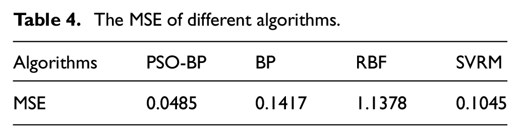
From Table 4, it can be known that the MSE value of PSO-BP neural network model positioning is 0.0485, and MSE of load position prediction for unoptimized BP neural network, RBF and SVRM is 0.057, 1.1378, and 0.1045, respectively. Prediction results of SVRM is better than BP and RBF. Of course, the prediction error of 0.1045 is not the best result. The advantage of SVRM is that it can get better results than other algorithms when processing small sample data sets, and it has excellent generalization ability. Moreover, the training time of SVRM is longer than BP and RBF, and its space consumption is mainly to store training samples and kernel matrix. For RBF neural network, it has strong nonlinear fitting ability. It can map very complex non-linear relationships, has global approximation capabilities, and has a fast convergence speed. But the prediction result of RBF neural network in this article is the worst. The reason for the analysis may be poor selection of parameters. If the SPREAD parameters of the RBF neural network are optimized, better prediction results may be obtained.

Research results show that the BP neural network optimized by the PSO algorithm has higher accuracy in predicting the position of the load. But this may not be the best result. For the research problem of the composite material load position recognition based on 2 × 2 optical fiber sensing in this paper, outputs of four optical fibers are used as the characteristic value, and the characteristic quantity is less. And for a 3 × 3 cm composite board, the imbalance of 500 samples will affect the prediction results of established PSO-BP model. In addition, some parameters of the PSO algorithm, such as population size, number of iterations, etc. will also affect the prediction accuracy. Therefore, in future research work, the performance of optical fiber sensors needs to be improved, and continuous experiments are needed to further optimize the performance parameters of the algorithm model or choose better algorithms such as deep learning to achieve better results.

Conclusion

The present article deals with the static load positioning of the optical fiber-composite structure based on the PSO-BP algorithm. The output strength of the four optical fibers is used as input, and the two-dimensional position coordinates are used as the output to establish a neural network model. The BP neural network model optimized by the PSO algorithm had high accuracy with R > 0.94, MSE = 0.0485. The performance is significantly better than the BP neural network model without optimization with R > 0.58, MSE = 0.1417. And compared with the traditional radial basis neural network with MSE = 1.1378 and support vector regression machine with MSE = 0.1045, the prediction accuracy is also higher. Research results show that PSO has better optimization capabilities, and PSO-BP neural network has better feasibility and higher accuracy in two-dimension positioning problems. The research in this paper provides a health monitoring method for optical fiber-composite structures. However, it does not mean that RBF and SVM are not good algorithms. They have a lot of advantages. We need to continue to explore, research, analyze, and improve, so that these algorithms can be better applied to various fields.

Future scope of work

Based on the PSO-BP algorithm, this paper constructed a type of model for optical fiber-composite structure load position recognition, and realized high-precision load position recognition. Based on the problems presented in the research on the load location method for composite structures, we will continue the following research in the future.

Collect as many data samples as possible to ensure the representativeness and balance of the samples;

Continue to improve our algorithm to improve the stability and prediction accuracy of the model.

The number of embedded optical fiber sensors and the area of composite materials can be increased to solve more complicated composite material load or damage location problems.

Improve the sensitivity of the optical fiber sensor and improve the characteristic of samples.

Try to apply more algorithms to the research of composite health detection, such as CNN, RNN, deep learn etc.

Footnotes

Acknowledgements

The authors are grateful to researchers Miaoqi Chen and Yuxuan Jiang for their valuable suggestions in the revision process of the article.

Declaration of conflicting interests

The author(s) declared no potential conflicts of interest with respect to the research, authorship, and/or publication of this article.

Funding

The author(s) disclosed receipt of the following financial support for the research, authorship, and/or publication of this article: This study was supported by Natural science foundation youth project of Jiangsu Province (Grant No. BK20190112), Ph.D. Project supported by the Jinling Institute of Technology (Grant No.jit-b-201814), School-level research fund incubation project of Jinling Institute of Technology (Grant No. jit-fhxm-2002), Ph.D. Project supported by the Jinling Institute of Technology (Grant No. jit-b-202012).

ORCID iD

LB Shen

References

Habib

Ezzedine

Tamer

. The efficiency of PSO-based MPPT technique of an electric vehicle within the city. Meas Control 2020; 53: 461–473.

Souza

Tarpani

. Distributed fiber optics sensing applied to laminated composites: embedding process, strain field monitoring with obr and fracture mechanisms. J Nondestruct Eval 2020; 39: 522–529.

Hassan

AlNedawe

Fakhri

. Embedded optical fiber link interferometer sensors for snapshot surface inspection using the synthetic wavelength technique. Appl Optics 2021; 60: 2339–2347.

Montoya

Castrillon

Perez

. In-flight and wireless damage detection in a UAV composite wing using fiber optic sensors and strain field pattern recognition. Mech Syst Signal Proc 2020; 136: 1–26.

Shan

Zhou

, et al. State sensing of composite structures with complex curved surface based on distributed optical fiber sensor. J Intell Mat Syst Struct 2019; 30: 1951–1968.

Kharwar

Verma

. Artificial neural network-based modeling of surface roughness in machining of multiwall carbon nanotube reinforced polymer (Epoxy) nanocomposites. FME Trans 2020; 48: 693–700.

Altan

Aslan

Hacıoğlu

. Real-time control based on NARX neural network of hexarotor UAV with load transporting system for path tracking. In: 2018 6th international conference on control engineering & information technology 2018, Istanbul, Turkey.

Califano

Chandarana

Grassia

, et al. Damage detection in composites by artificial neural networks trained by using in situ distributed strains. Appl Compos Mat 2020; 27: 657–671.

Wang

Liu

Yang

, et al. Quantitative monitoring method of composite material structure delamination damage based on neural network. Fiber Compos 2020; 37: 50–54.

10.

Zhang

Tong

, et al. Composite material impact location detection technology based on BP algorithm and FBG sensing. Laser Technol 2022; 46: 320–325

11.

Ren

. Application analysis of particle swarm optimization bp neural network algorithm in highway deformation prediction. Electron Meas Technology 2020; 43: 80–84.

12.

Altan

Karasu

Zio

. A new hybrid model for wind speed forecasting combining long short-term memory neural network, decomposition methods and grey wolf optimizer. Appl Soft Comput J 2021; 100: 1–20.

13.

Kesarwani

Verma

. Grey integrated multiobjective-particle swarm optimization (MOPSO) for Machining assessment and predictive modeling of Cutting Forces generated during Polymer nanocomposite Drilling. In: E3S Web of Conferences 309, 01222, 2021, ICMED 2021.

14.

Karasu

Altan

Bekiros

, et al. A new forecasting model with wrapper-based feature selection approach using multi-objective optimization technique for chaotic crude oil time series. Energy, 2020; 212: 1–12.

15.

Gomes

Diniz

da Cunha

Simões

, et al. Design optimization of composite prosthetic tubes using GA-ANN algorithm considering Tsai-Wu failure criteria. J Fail Anal Preven 2017; 17:740–749.

16.

Vosoughi

GeristNew

. hybrid FE-PSO-CGAs sensitivity base technique for damage detection of laminated composite beams. Compos Struct 2014; 118: 68–73.

17.

Liu

Zhao

Bai

. Strain transfer analysis of simplified interface of embedded optical fiber smart composites material. Mater Rep 2021, 35(20): 20161–20165.

18.

Wang

. Research on the prediction of learning performance based on PSO-BP Network. J Anyang Normal Univ 2021; 2: 41–45.

19.

Chen

Shi

, et al. RFID indoor positioning algorithm based on PSO optimization. Commun Technol 2018; 51: 2069–2074.

20.

Chen

Zhao

, et al. Damage identification method of continuous beam bridge based on strain and PSO-BP neural network. J Saf Environ 2017; 17: 2093–2098.

21.

Wang

Shi

, et al. Indoor positioning technique by combining RFID and particle swarm optimization-based back propagation neural network. Optik 2016; 127: 6839–6849.

22.

Wang

Hadi

Christos

, et al. A new RBF neural network-based fault-tolerant active control for fractional time-delayed systems. Electronics 2021; 10(12): 45–54.

23.

Feng

. Processing method of EMD endpoint effect based on SVRM extension. Vibroeng Proc 2020; 35: 134–142.

24.

. Large-scale landslide displacement rate prediction based on multi-factor support vector regression machine. Appl Sci 2021; 11(4): 16–23.

A static load position identification method for optical fiber-composite structures based on particle swarm optimization- back Propagation neural network algorithm

Abstract

Keywords

Introduction

Experimental details

Methodology

BP neural network

PSO algorithm

Establishment of PSO-BP neural network model

Data sets division and normalization

Parameter settings of BP neural network

Parameter settings of PSO algorithm

Results and discussion

BP and PSO-BP neural network prediction

Comparison with other algorithms

Conclusion

Future scope of work

Footnotes

Acknowledgements

Declaration of conflicting interests

Funding

ORCID iD

References