
Abstract
The static synchronous multi-pressure sensing system (SMPSS) test technique is one of the most conventional techniques used in a wind tunnel. In SMPSS tests, wind pressure sensors are prone to take off leading to missing segment data. This study has predicted single, short-term, and long-term wind pressures by a one-dimensional convolutional neural network based on empirical mode decomposition (EMD-1DCNN). The effectiveness of the EMD-1DCNN model in predicting single, short-term, and long-term wind pressures on bluff bodies has been discussed. It was found that the EMD-1DCNN model had a better performance in predicting single wind pressures compared with the DNN and LSTM models. It was also found that both the DNN and LSTM models failed to predict short-term wind pressures, while the EMD-1DCNN model was effective in addressing this problem. The EMD-1DCNN model extracted the spatial feature between wind pressure sensors and its surrounding sensors to predict long-term wind pressures with high accuracy. The effects of data length used for training the EMD-1DCNN model on the accuracy of prediction were also discussed. It was concluded that 1% datasets (500 samples) were enough for predicting long-term wind pressures with high efficiency. This study has not only presented a way to predict missing data of wind pressures using the EMD-1DCNN model but provided recommendations for the EMD-1DCNN model used for different conditions.
Keywords
Introduction
With the rapid development of economy and society in recent years, the demand for high-rise buildings and long-span bridges has remarkably increased. Super high-rise buildings have been built worldwide, such as Burj Khalifa, Shanghai Tower, and Petronas Twin Towers, etc., as new landmarks of cities. These high-rise and slender buildings are wind-sensitive structures, which makes them more sensitive to wind excitation than low-rise buildings. It is well known that wind loads could have a significant impact on the safety of a structure and a wind tunnel test is one of the most reliable ways to evaluate wind loads acting on structures.1–3 There are two conventional wind tunnel test techniques in estimating wind loads on structures, namely the high-frequency base balance (HFBB) and the static synchronous multi-pressure sensing system (SMPSS) test techniques. 4 The HFBB technique uses a force balance at the base of a test model to measure aerodynamic forces acting on the model. This technique is simple and cost-saving in evaluating overall aerodynamic forces on a test model. Although the HFBB considers the linear mode shape, it cannot acquire wind pressure distribution on a test model. An alternative method, namely the SMPSS technique, can measure pressures acting on a test model, which can be used for evaluating overall and the local aerodynamic forces by means of integrating wind pressures along with the height of the test model. It can estimate non-linear mode shapes and present more information than the HFBB approach. However, there are some shortcomings in the SMPSS technique used in a wind tunnel. The technique utilizes many pressure sensors to estimate aerodynamic forces, which is costly and time-consuming. Moreover, it is difficult to fix pressure sensors for a test model with a complicated geometric configuration. More importantly, pressure sensors installed on a test model would be prone to take off during experimental setups and wind tunnel tests, which can lead to data missing and lower accuracy in evaluating the aerodynamics and aeroelasticity of structures. Therefore, it is of great importance to predict wind pressures on a missing point.
Recent evidences suggest that deep learning methods, as a data-driven approach, 5 are effective in addressing problems in wind engineering and have been utilized in various fields, such as bridge engineering 6 and structural health monitoring 7 etc. Azad et al. 8 have utilized a non-linear autoregressive neural network to predict long-term wind speeds and found that it had a better performance than traditional methods (e.g. adaptive neural fuzzy inference systems, support vector machines, and auto-regression models). Zhang et al. 9 have built a Predictive Deep Boltzmann Machine (PDBM) model to extract the higher-level features of raw wind pressure data to predict hour-ahead and day-ahead wind speed with non-linear and non-smooth functions. Khodayar et al. 10 have presented a deep neural network architecture with stacked auto-encoder (SAE) or denoising auto-encoder (SDAE) to predict short-term wind speeds. In order to improve the accuracy of prediction, rough neural networks were integrated into SAE and SDAE, which has presented great robustness for wind speed forecasting. It was also found that, compared to classical deep learning neural networks and traditional models, the SDAE and SAE had a lower evaluation index of RMSE and MAE. Wind uncertainties would increase the difficulty of capturing wind features. To address this problem, Khodayar et al. 11 have proposed an interval deep belief network (IDBN) based on interval probability distribution learning (IPDL) and fuzzy type II inference system, which could perform the supervised regression to evaluate wind speed. In structural wind engineering, Jin et al. 12 have used a fusion convolutional neural network (FCNN) to predict the velocity field around a circular cylinder based on fluctuating pressures. The results showed that CFD calculations of the velocity field were in close agreement with the FCNN prediction, indicating that deep learning models were effective to learn flow regimes around cylinders. Oh et al. 13 have utilized wind pressure data in the frequency domain and top-level wind-induced displacement in time and frequency domain to predict the wind-induced response of high-rise buildings using a convolutional neural network (CNN). Moreover, strain data was used for the CNN model to evaluate the effectiveness of the CNN performance. Raissi et al. 14 have proposed a deep neural network embedded in structural dynamic motion to predict accurately structural parameters (e.g. damping and stiffness) and an entire time-dependent pressure field via using scattered data of a velocity field and structure’s motion in space-time. Jin et al. 15 have utilized bidirectional gated recurrent units to extract time sequences of coefficients on the first few orthogonal decomposition modes to obtain a time-resolved flow field around a circular cylinder. In addition, in order to validate the effectiveness of the proposed approach, two experimental datasets with different Reynolds numbers were utilized to analyze the relationship between the velocity-time sequence and the spatial distribution of velocity. Snaiki and Wu 16 have presented a knowledge-enhanced deep learning model to simulate the wind field inside a tropical cyclone boundary-layer based on the storm parameters. Tian et al. 17 have used a deep neural network to predict mean and peak wind pressure coefficients on the surface of a scale model building. Furthermore, to improve predicted accuracy in peak coefficients, wind pressure data from various wind directions and terrain roughness was fed into a two-step nested deep neural network procedure, and the result indicated that the CNN presented a higher accuracy. Zheng et al.18–20 have proposed a novel CNN model that is powerful in tackling the problem of wind pressure. In the above algorithms, CNN, as a data-driven method, doesn’t need more assumptions and automatically adjust training parameter according to the data. More importantly, CNN can capture the complex changes of wind pressure affected by many factors, such as wind speed and turbulent flow.
In addition, to better understand the variation of wind pressure. Empirical mode decomposition (EMD) is utilized to decompose the wind pressure before CNN model. EMD, as a time series analysis method, can effectively extract a set of intrinsic mode functions (IMFs) to describe the condition of wind pressure. Duan et al. 21 have used a hybrid EMD-SVR model for predicting the short-term wave height. Compared with an auto-regressive model, single SVR model, and EMD-AR model, the result showed that the EMD-SVR had a good model performance and low mean square error to handle the short-term prediction of wave height. Li et al. 22 have proposed coupling EMD and a long short memory time to predict missing measured signal data. The experiments showed that the proposed method exhibited excellent performance in predicting missing data and fitted more microscopic changes of measured values.
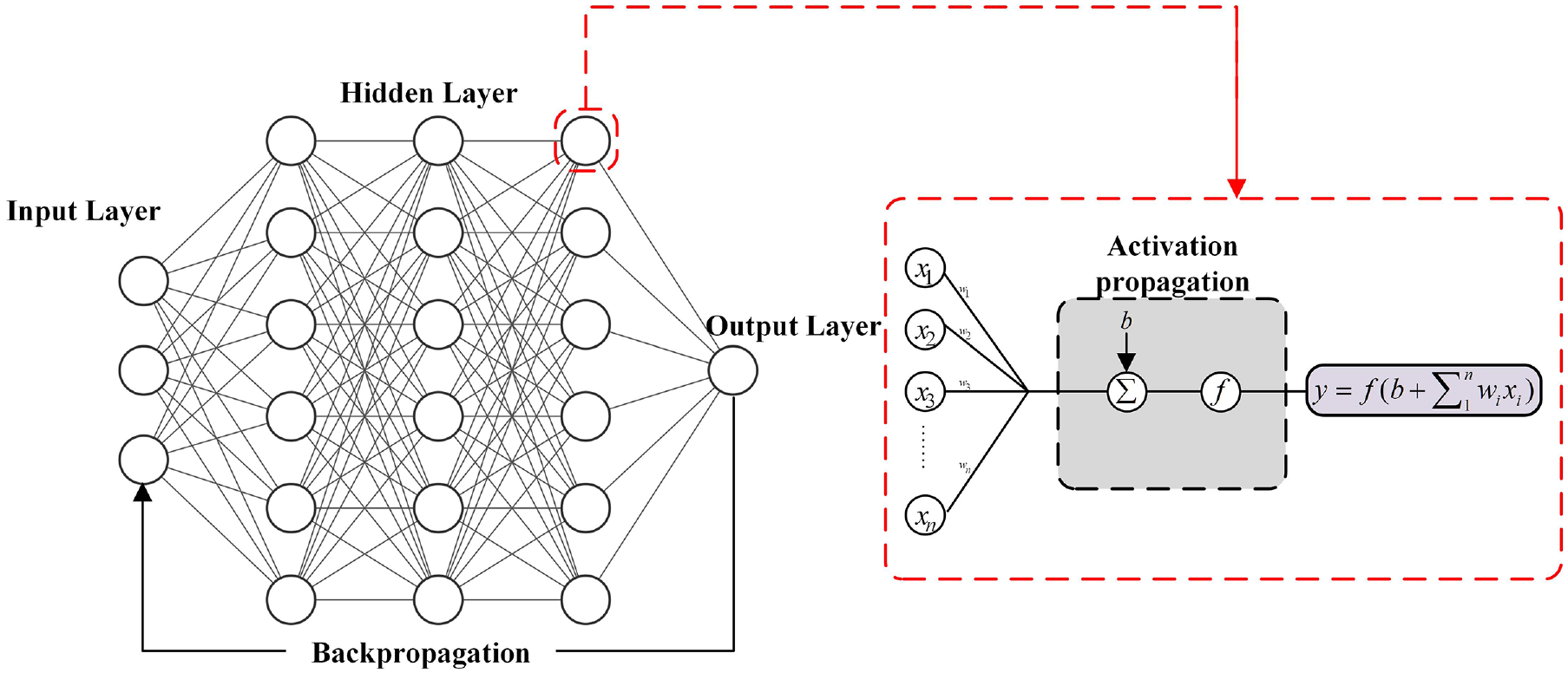
In recognition of the strong abilities of EMD to decompose wind pressure data and 1DCNN to capture the spatial correlations of wind pressure. An EMD-1DCNN model is proposed in this study for the imputation of missing measured signal data where the EMD component can decompose a non-stationary and non-linear wind pressure into physically meaningful signals that represent various time scales. Then, using a 1DCNN component, as a feature extractor, extract the spatial features of decomposed time series through different convolutional kernels. Finally, the spatial features are fed into fully connected layers to predict missing data.
In addition, the missing segment predictions include three ways, namely single, short-term, and long-term wind pressure prediction. Single data missing represents that a sampling point is missing, short-term represents several sampling points is missing, and long-term data missing represents a large amount of sampling point is missing. With the increasing number of missing data, a hybrid EMD-1DCNN model also presents an outstanding performance compared with traditional deep learning methods (DNN, LSTM).
Wind pressure prediction methods
Wind pressure prediction using deep learning methods
Deep learning models, inspired by the human biological nervous system, 23 are presented in this section. Classical deep learning models, including the one-dimensional convolutional neural network (1DCNN), long short-term memory (LSTM), and deep neural network (DNN), have exhibited outstanding performance in capturing the feature of inherent nonlinearities of the system. For example, the 1DCNN was utilized to predict dominant wind speed and direction for the temporal wind dataset. 24 Bidirectional LSTM has been utilized to predict sensory data successfully in the wireless sensor network with high quality. 25 Besides, The DNN has performed precisely a prediction in mean and peak wind pressure coefficients on the surface of a scale model building. 17
Long short-term memory
Long short-term memory (LSTM) is an improved recurrent neural network (RNN) and has a long history in speech recognition. This model could easily address the problem in time series predictions and has been extensively applied to deal with long-range dependencies of sequential data through the memory unit to accumulate the information. 26
According to Figure 1, each LSTM unit has a cell state
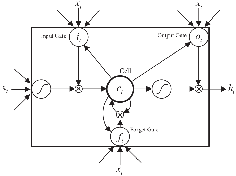
Long short-term memory unit.
As mentioned previously, an LSTM could accumulate significant information for the final result during the data analysis and find and exploit long-range contexts via the feedback process. The corresponding update equations of LSTM, as follows.


where
Deep neural network
Deep neural network (DNN) developed by human biological nervous systems is widely used to build the mapping relation of complex mathematics between input and output data. A DNN is one of the state-of-the-art deep learning algorithms, presenting excellent performance to extract high-level features from any inherent non-linear systems, including raw wind pressure data in wind engineering. The architecture of DNN (Figure 2) includes input layers, hidden layers, and output layers. Each hidden layer has many neurons, which are the most basic elements in a DNN model. Furthermore, there are two primary operations, including feedforward, and backpropagation, in a DNN model. During a feedforward propagation, the input data is delivered to a DNN model to obtain predicted output data via equation (7). Besides, Error-values are determined by comparing the actual output data with the predicted data for updating the weight matrix and bias vector based on a gradient-descent optimizer algorithm during backpropagation.
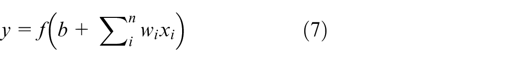
Architecture of deep neural network.
where
Framework of the proposed method
Architecture of EMD-1DCNN
As shown in Figure 3,
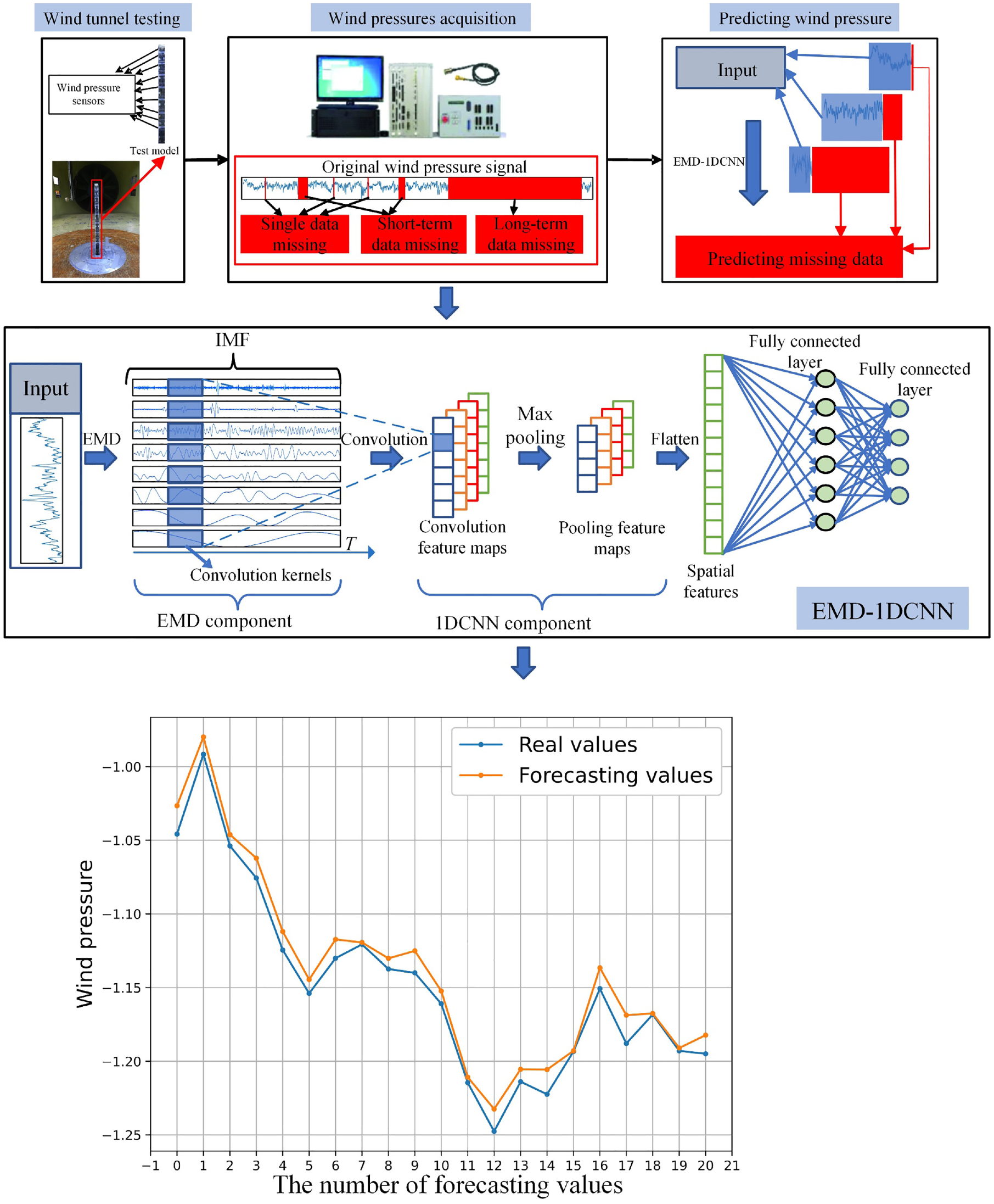
Architecture of the proposed EMD-1DCNN model.
Empirical mode decomposition component
Empirical mode decomposition (EMD) was proposed by Huang et al.
27
Compared with Fourier decomposition and wavelet decomposition using a basis function, EMD is utilized to decompose signals with non-stationary and non-linear features according to the time scale characteristics. In addition, due to wind pressure with a non-stationary characteristic, EMD has great advantages in analyzing it and eliminate noises of wind pressure data. Specifically, the wind pressure data
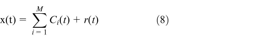
Figure 4 shows the corresponding IMF components of wind pressure data.
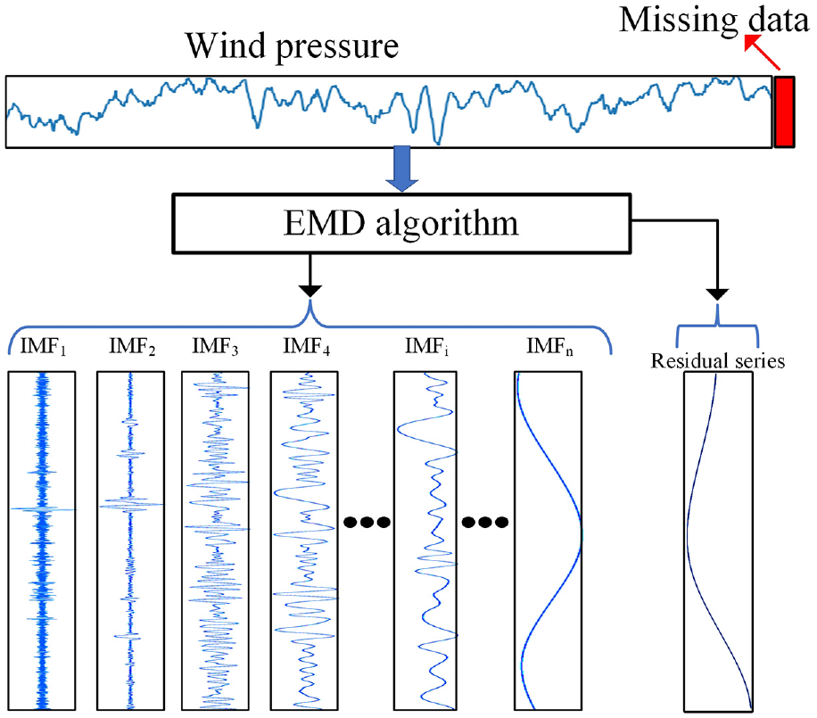
IMF of wind pressure using EMD algorithm.
One-dimensional convolutional neural network component
A one-dimensional convolutional neural network (1DCNN) has been utilized to analyze structural damage detection 30 and wind prediction. 24 The 1DCNN mainly includes three layers, convolutional layers, pooling layer, and fully connected layers, respectively, as shown in Figure 5.
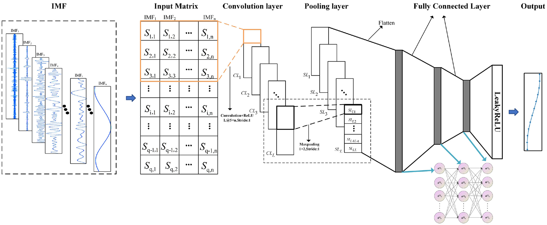
Architecture of 1DCNN component.
In Figure 5, every length of
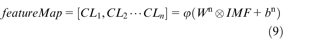
where
The pooling layers following the convolutional layers (Figure 5) are used to significantly reduce the computational complexity by decreasing the dimension with width and height of the output neurons of convolutional layers. The maximum pooling layers are expressed by

where
Experimental setups
In this subsection, model parameters and algorithm implementation are described. To estimate the performance of deep learning models, four statistical indicators are adopted.
Model parameters
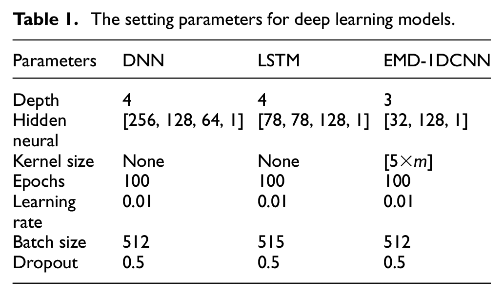
To improve the accuracy and efficiency of deep learning models, there are some implementation details to perform during the model training phase. To handle the overfitting problem of deep learning models, the dropout method could be adopted, and the value is set as 0.5. Initial learning rate is set to 0.01, and batch size is set to 512. Adam optimization is applied to optimize the network architecture that makes the learning rate decrease with increasing of epochs number. Moreover, these models are programmed under Pytorch framework that is an open-source neural network, which runs on a high-performance workstation with two Intel Xeon E5 processors and one Nvidia computable GPU unit.
All parameters of deep learning models are as follow:
DNN: The DNN, including four layers that are fully connected neural networks with ReLU activation function, is used for training; Each layer has 256, 128, 64, 1 neurons.
LSTM: The LSTM with one layer of LSTM cells (78 dimensional hidden states) is adopted for training. Following the LSTM cells are two fully connected networks that have two layers with 128 and 1 neurons, which generates the final prediction.
EMD-1DCNN: wind pressure data can be decomposed into several IMFs and one residual series, and these data series are fed into the 1DCNN model where the number of kernels is 32. The size of convolutional kernels is 5×
Table 1 shows the setting parameters of deep learning models. Each model are setting to similar epochs, learning rate, batch size, and dropout, which can equally compare the performance of different algorithms.
The setting parameters for deep learning models.
Algorithm implementation
Input-output matrix
Previous studies have shown a time correlation between the state of the wind pressure data at the previous time and the state at the next time.
31
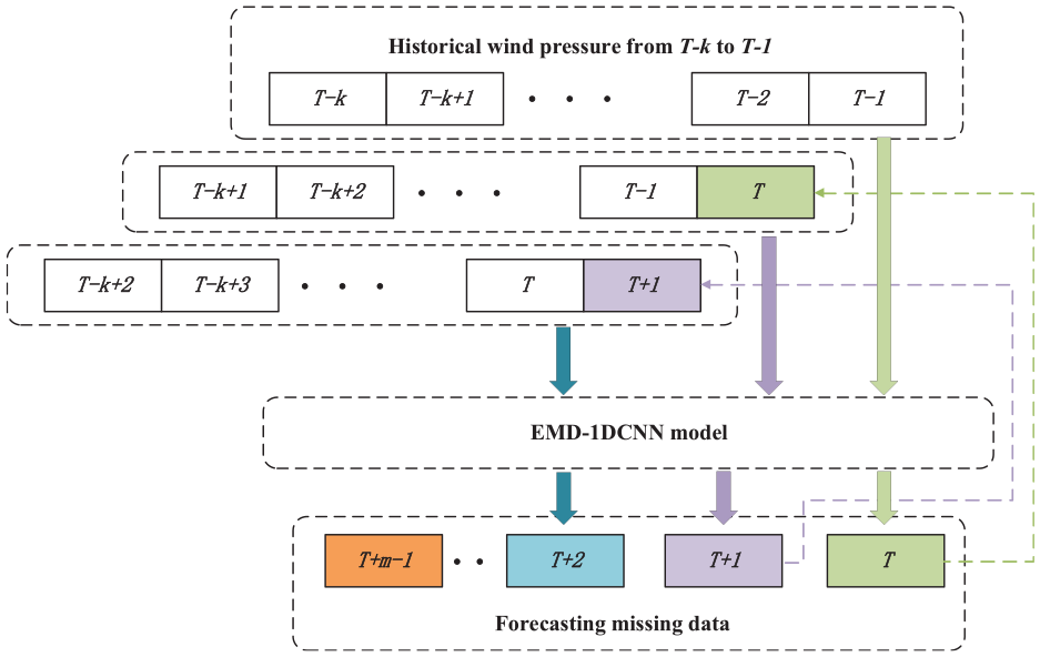
Thus, EMD-1DCNN extracts features of wind pressure at previous time to predicting missing data via a strongly non-linear learning ability. In Figure 6, the input matrix
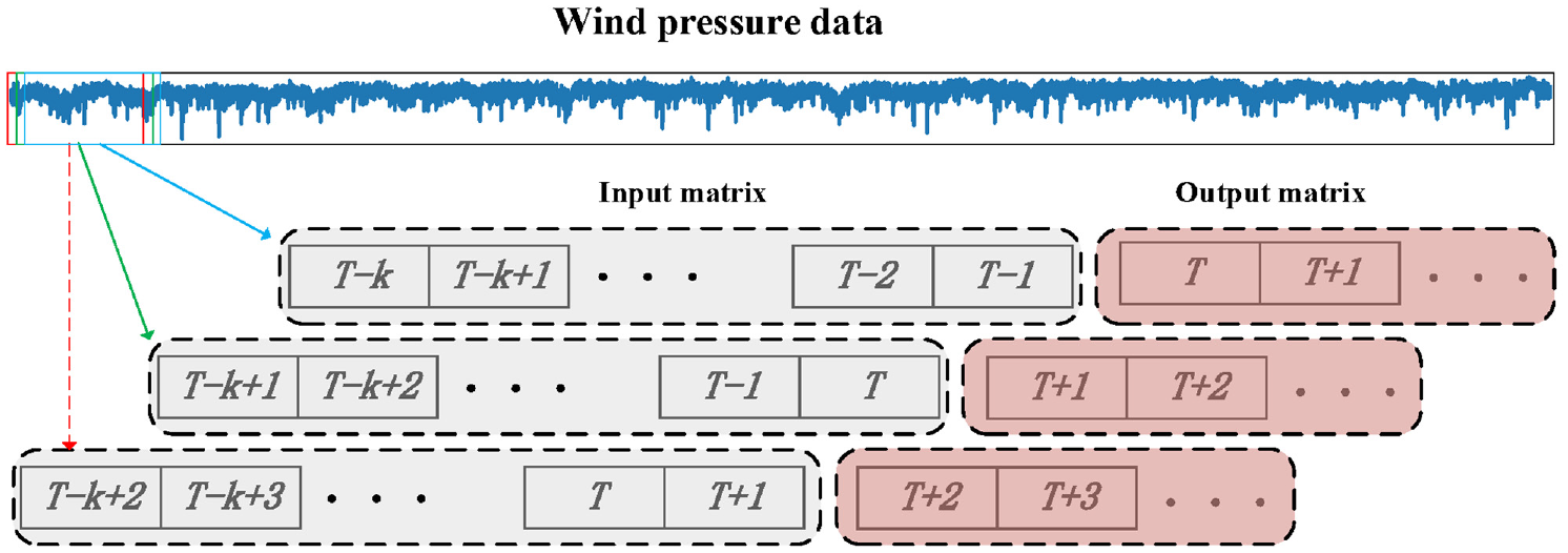
Input-output matrix for the proposed EMD-1DCNN model.
Schematic diagram of the proposed model
The proposed EMD-1DCNN is implemented in a high-performance workstation. The available dataset is split into the training and testing sets according to a heuristic rule, which adopts a ratio of 8:2. 32 For the training process of the proposed model, taking a backpropagation through time (BPTT) algorithm to minimize mean squared errors over all input simple (Figure 7).
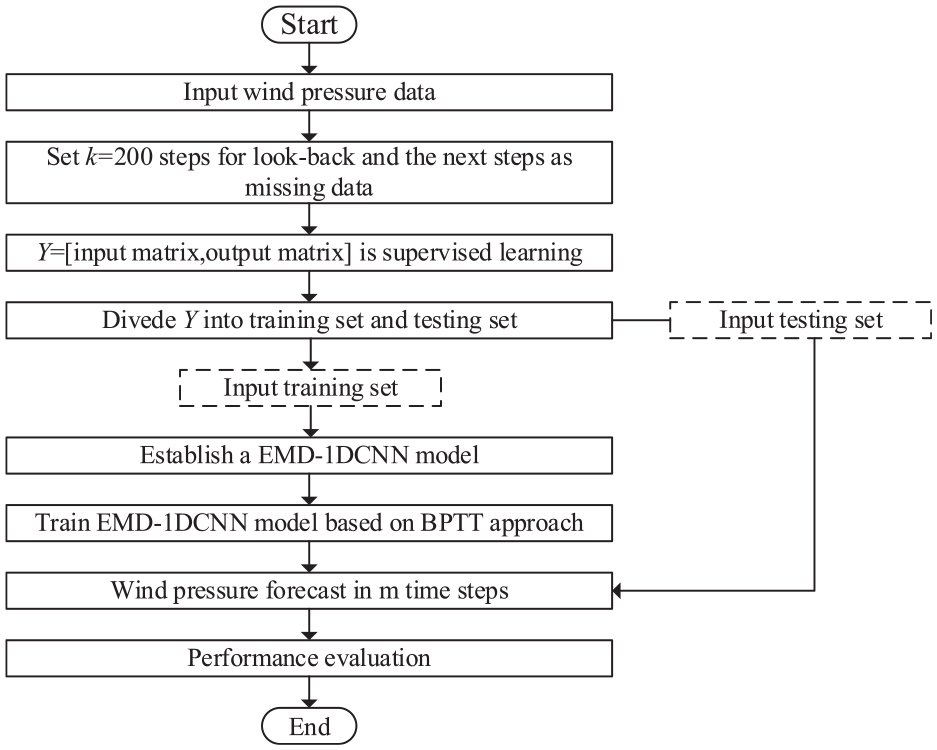
Schematic diagram of the proposed EMD-1DCNN model.
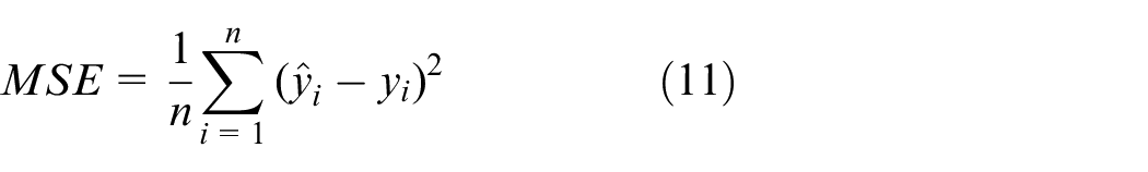
Evaluation criteria
To estimate the performance of deep learning models under the different forecasting situations, four evaluation criteria including mean squared error (MSE), root mean squared error (RMSE),
33
and mean absolute error (MAE),
34
are used to represent the error degree between the actual values and predicted values. Furthermore, the smaller values of the MSE, RMSE and MAE show better forecasting performances for different deep learning models. R-squared
35
represents the fitness of the model for the observed data. When the value of
where
Experimental results and discussion
Datasets
Pressure measurements for a bluff body were performed at the CLP Power Wind/Wave Tunnel Facility of the Hong Kong University of Science and Technology. The dimensions of the wind tunnel were 29.2 m (length) × 3 m (width) × 2 m (height). In addition, Wind pressure data was collected by a synchronous multi-pressure sensing system (SMPSS). The dimensions of the test model were 50.8 mm (D) × 50.8 mm (D) × 915 mm (H) with an aspect ratio (H/D) of around 18:1. There were 162 pressure sensors distributed on nine levels of all four faces of the test model. The terrain category II defined in the AS/NZS 1170.2:2002 was simulated in the wind tunnel by adjusting roughness elements and spires in the upstream of the test section, and a hot-wire anemometer was utilized to measure the mean wind speed and flow turbulence intensity. During the test, only normal flow incidence on the prism was considered, and the reduced wind speeds
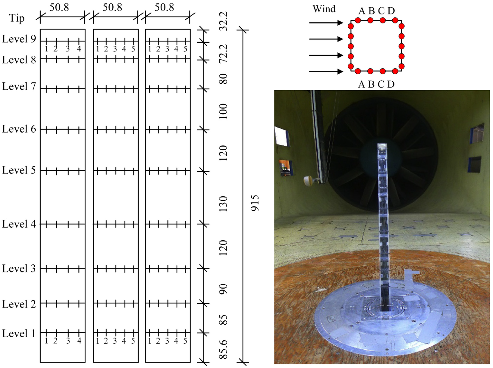
Distribution of pressure sensors (units: mm). 1
In the static SMPSS pressure measurement, the sampling duration and frequency were 100 s and 500 Hz, respectively; as a result, each pressure dataset included 50,000 numbers. In order to understand the features of wind pressure datasets, some datasets were described by four statistical indicators, including mean, standard, max, and min in Table A1. For simplicity, “B11” denoted the first point of level 1 for the backward face. “F11” represented the first point of level 1 for the windward face. “L11” stood for the first point of level 1 for the lateral face.
Figure 9 shows the time series of wind pressure datasets collected sensors installed in the test model for 100 s. From the pictures, these wind datasets have a strongly non-linear feature. Thus, traditional methods (such as mean imputation and regression imputation) are utilized to predict the wind pressure with missing, having a lower forecasting accuracy.
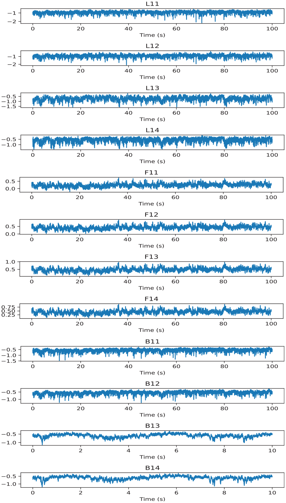
Part of wind pressure acting on the test model.
Wind pressure prediction with single data missing
The input-output pairs for a training and testing process are described in Figure 10. For wind pressure forecasting with single data missing, a time series consisting of a time sequence
Input-output pairs for predicting single data missing.
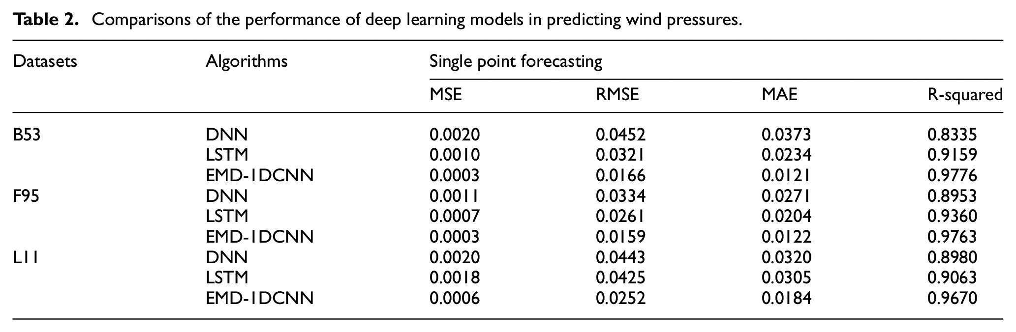
In this study, three represent datasets (B53, F95, L11) located in different faces and levels are selected to verify the proposed method. In Table 2, for the B53, compared with DNN and LSTM models, the proposed EMD-1DCNN model has a preferable performance in single data missing. Specifically, the mean absolute error (MSE) values are 0.0003, which are the smallest compared with the DNN and LSTM models. For the F95, MSE, RMSE, MAE, and R-square are all obtained from the EMD-1DCNN model, with values of 0.0003, 0.0159, 0.0122, and 0.9763, respectively. For the L11, the condition is similar to that in the B53 and F95 datasets of the building. To be specific, the lowest MSE value is 0.0006, obtained from the EMD-1DCNN model, and the worst MSE is obtained from DNN model, with a value of 0.0020, indicating that the EMD-1DCNN model validly reduces the forecasting error to a great extent.
Comparisons of the performance of deep learning models in predicting wind pressures.
To observe the training process of the proposed method, Figure 11 shows the loss curve for different points, including B53, F95, L11, using the EMD-1DCNN model. The horizontal axis signifies epochs number and the vertical axis represents loss value. The loss value is very low, and the curve is very smooth, indicating the model achieves an excellent fitting ability.
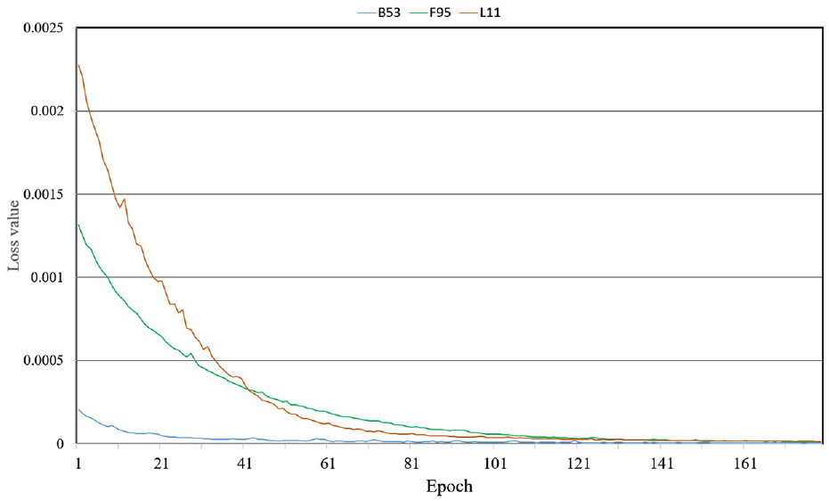
Loss curve based on EMD-1DCNN model.
To further illustrate the distinction between forecasting values and predicted values based on the testing dataset in DNN, LSTM, and proposed EMD-1DCNN models, a random segment with 2 s of predicted result (B53, F95, L11) are shown in Figures 12 to 14.
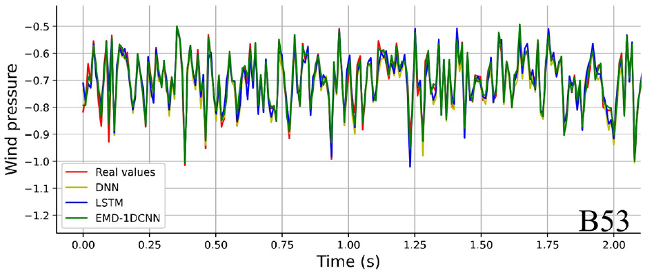
Comparisons of prediction capabilities for different models (B53).
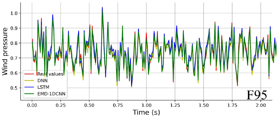
Comparisons of prediction capabilities for different models (F95).
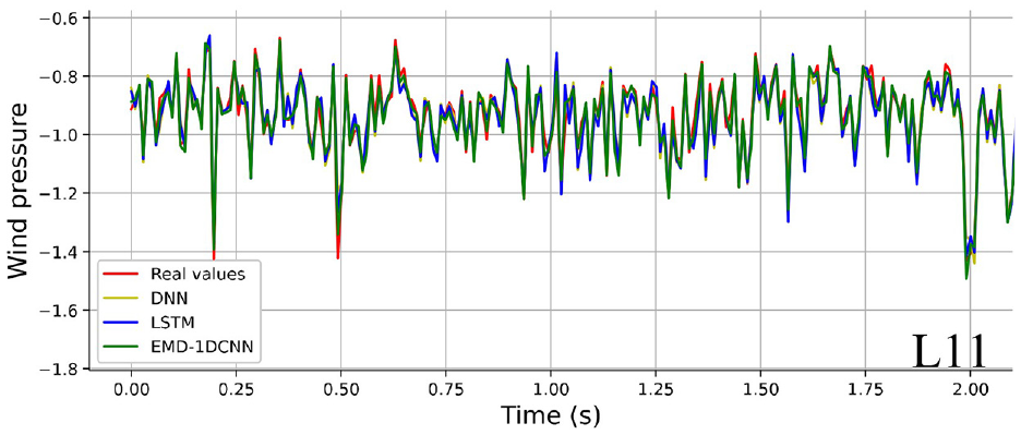
Comparisons of prediction capabilities for different models (L11).
Compared with DNN, LSTM models, Figures 12 to 14 indicate that the EMD-1DCNN presents an excellent forecasting capability for single data missing and maintains the shape of the original curve well.
In Figure 15, the deviation (B53, F95, L11) between the forecasting and actual values in the scatter chart suggests that the predicted values are close to actual values using the EMD-1DCNN model. To be specific, for F95, the
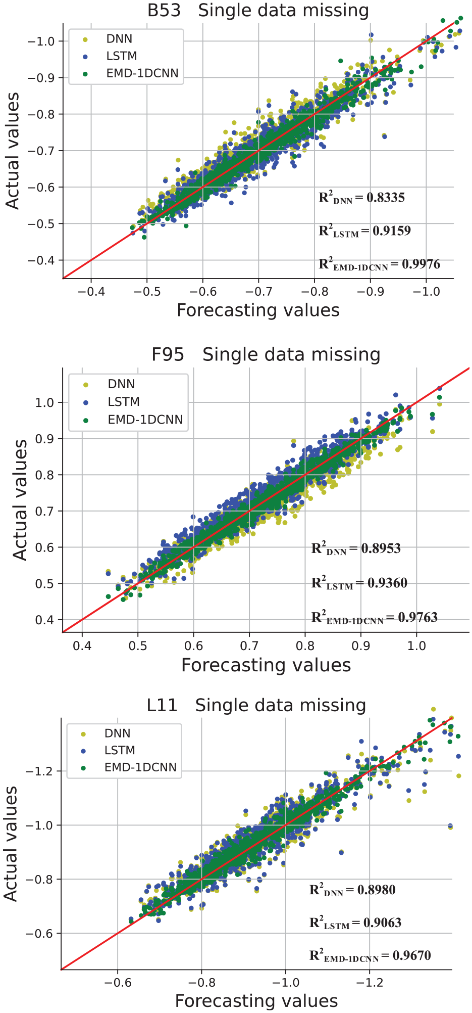
Scatter chart of different datasets (B53, F95, L11).
Wind pressure prediction with short-term data missing
For the short-term wind pressure prediction, the time series
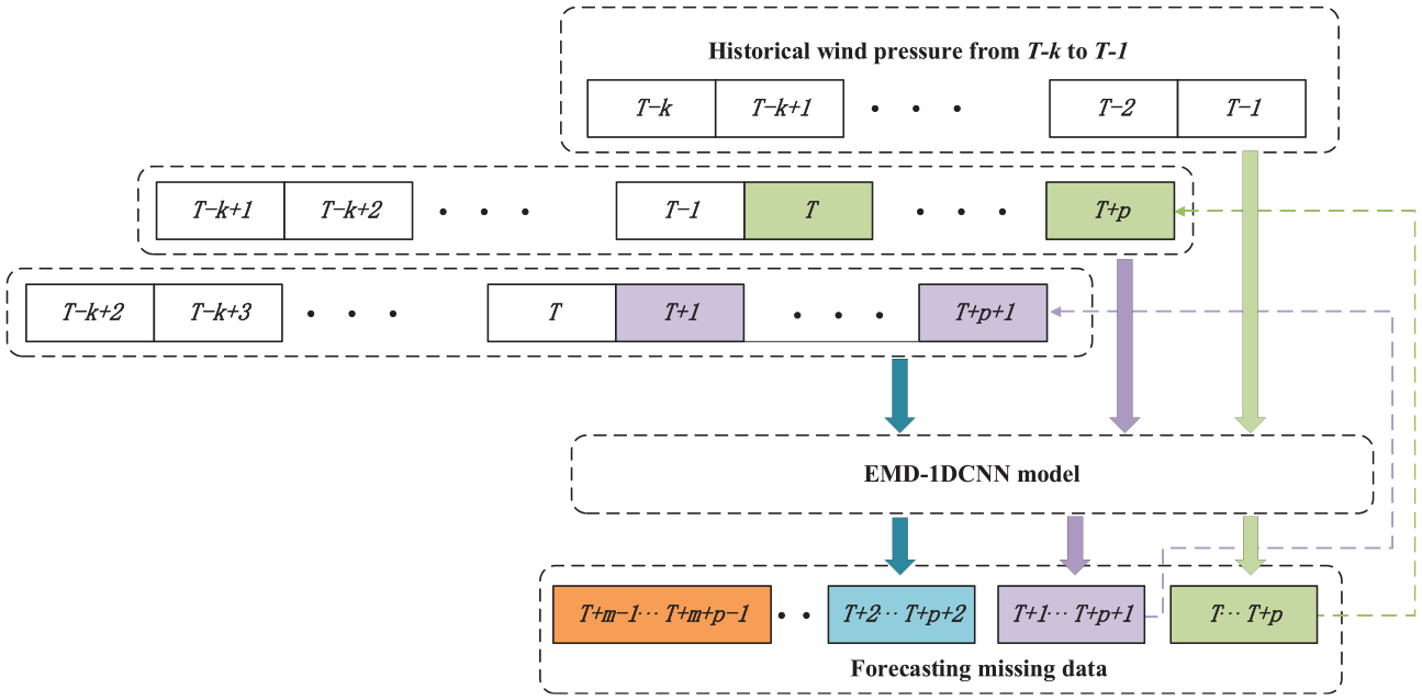
Samplings from the original time series.
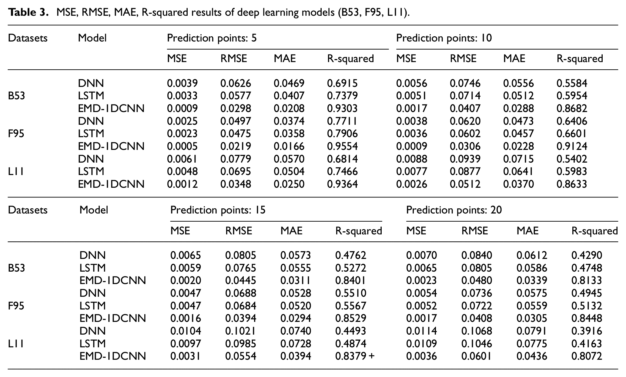
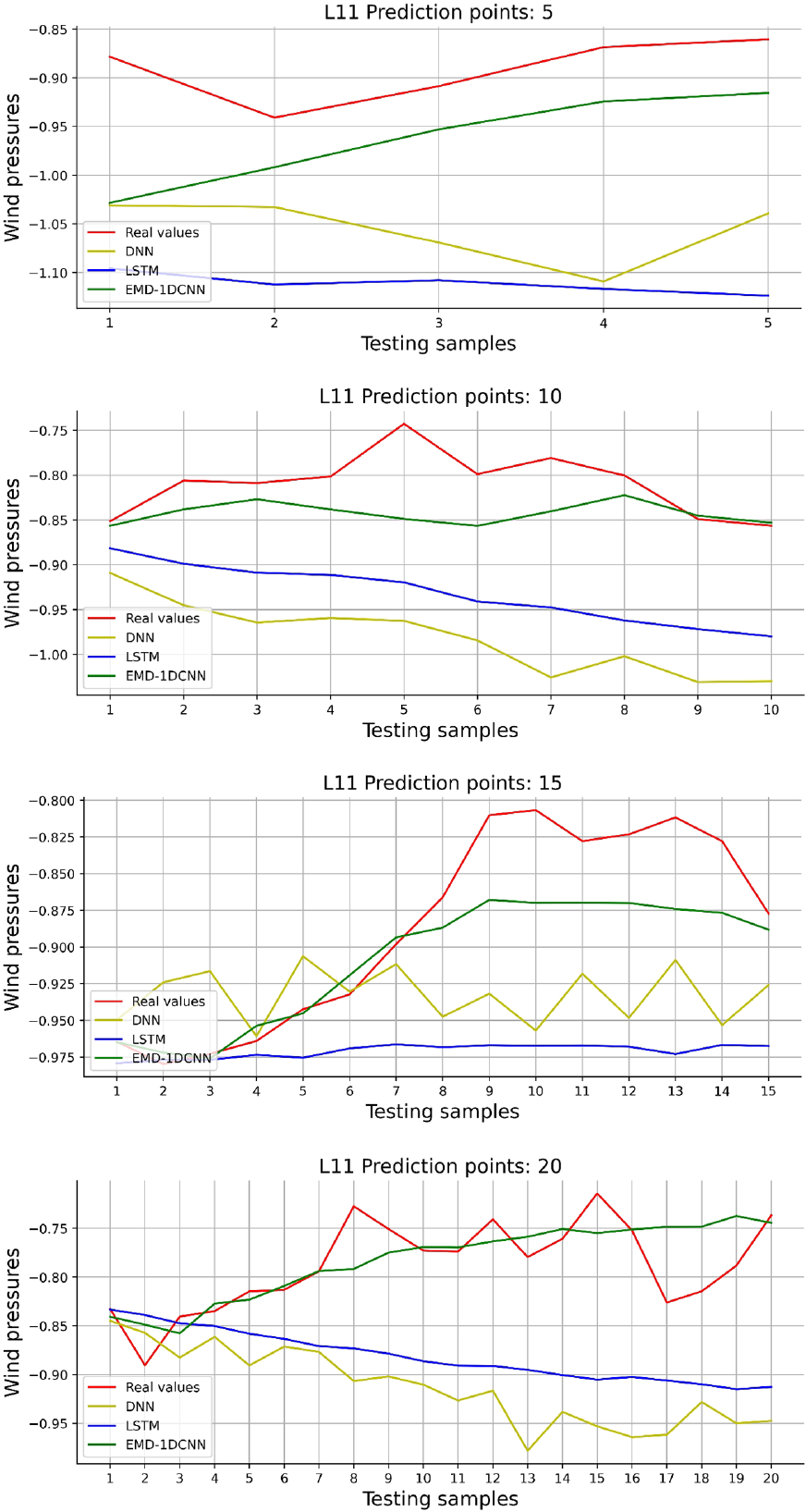
Table 3 summarizes the experimental results of short-term wind pressure prediction based on the testing datasets calculated by the used DNN, LSTM, and EMD-1DCNN models. Consequently, it is found that the EMD-1DCNN can be efficiently used for wind prediction, whether in 5, 10, 15, 20-points prediction. Specifically, for the B53, the RMSE values are 0.0298, 0.0407, 0.0445, 0.0480 in short-term prediction, which are the smallest compared with the DNN and LSTM models. For the F95, with the increasing number of steps ahead, the R-squared values of the deep learning models decrease gradually, indicating that the ability of models’ prediction becomes weaker and weaker. The decreasing trend of R-squared values of the EMD-1DCNN model is remarkably smaller than DNN and LSTM models. The result shows that the EMD-1DCNN presents a preferable performance in 5, 10, 15, 20-points prediction. For the L11, the EMD-1DCNN model presents an outstanding prediction ability. To be specifical, the MSE, RMSE, MAE, and R-square are all obtained from the EMD-1DCNN model in 5-points prediction, with values of 0.0012, 0.0348, 0.0250, and 0.9364, respectively, confirming the conclusion that the LSTM and DNN models fail to predict short-term wind pressures on structures.
MSE, RMSE, MAE, R-squared results of deep learning models (B53, F95, L11).
To further show that the deviation degree of real values and predicted values based on the testing dataset, a random segment of predicted results (B53, F95, L11) are shown in Figures 17 to 19.
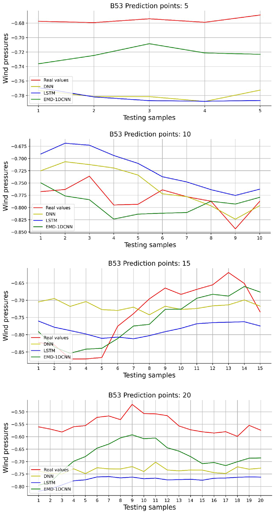
Comparisons of short-term wind pressure prediction using deep learning models (B53).
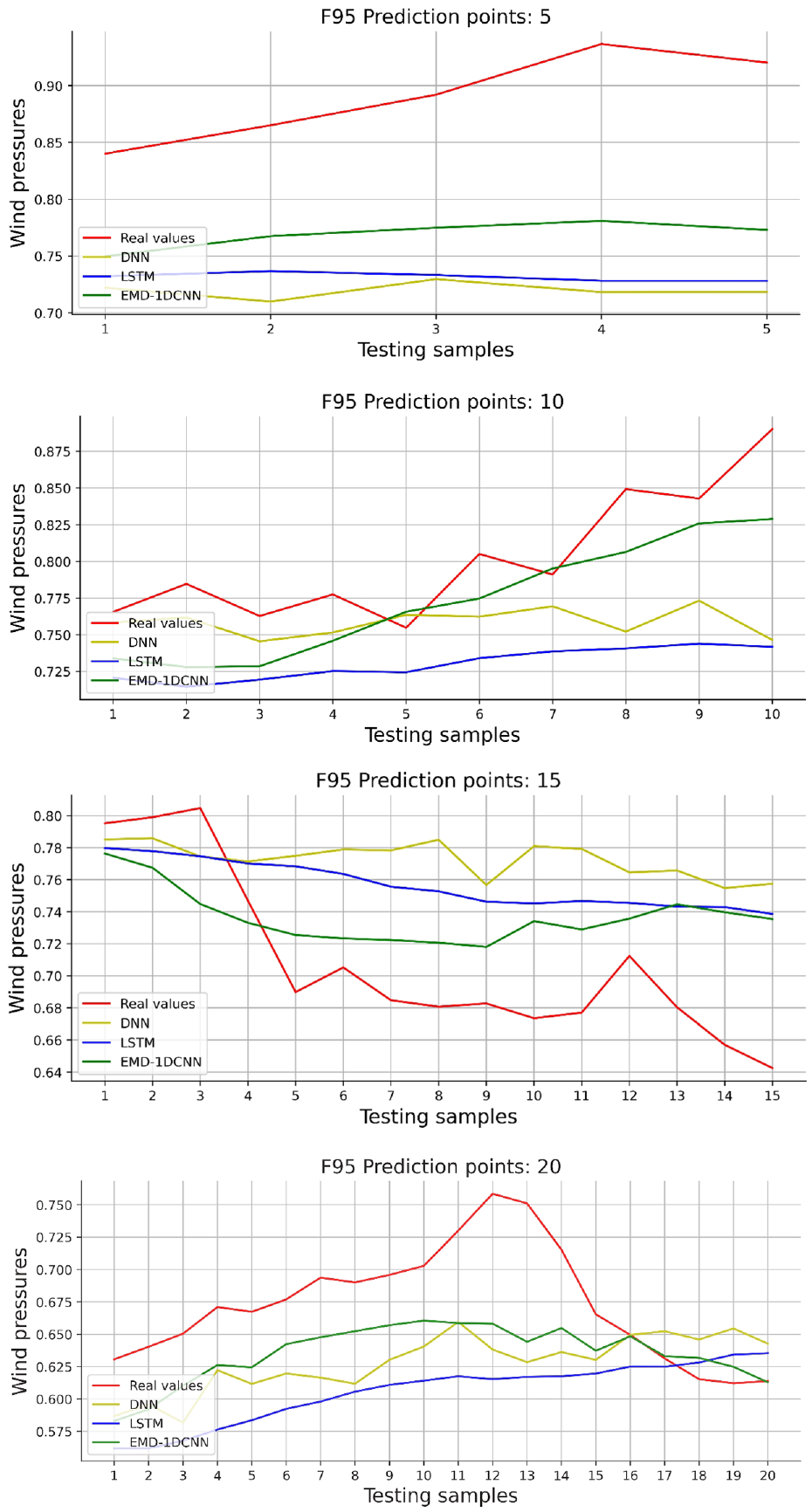
Comparisons of short-term wind pressure prediction using deep learning models (F95).
Comparisons of short-term wind pressure prediction using deep learning models (L11).
Figures 17 to 19 both the magnitudes and trends of DNN and LSTM models predicted values are far from real values with the increase of the forecasting length. Moreover, the trend line of DNN and LSTM models have greatly different from the actual trend line. However, the EMD-1DCNN model predicts values that are close to real values, and the predicted trend line is similar to the actual trend line. Because the EMD can decompose wind pressure into several IMFs and one residual, showing more internal relationships between time series. Thus, the 1DCNN model can effectively extract features of the decomposed sub-series for getting a predicted result.
Wind pressure prediction with long-term data missing
Although wind pressure with single and short-term data missing based on EMD-1DCNN model has a good predicted capacity, the
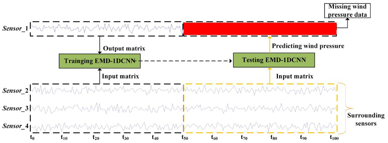
Predicting long-term data missing using EMD-1DCNN.
The first 50 seconds datasets of surrounding sensors (
In the study, three representative datasets (F93, B53, and L91) and the corresponding surrounding sensors (the first 50 s) are selected in Table 4, which are fed into EMD-1DCNN model to predict the missing data (remaining 50 s).
Input-output matrix of datasets (F93, B53, and L91).

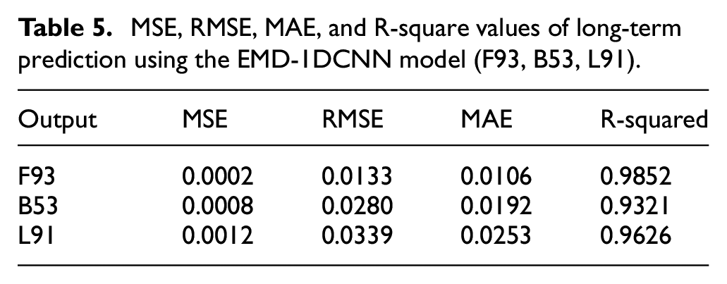
Table 5 shows the result of long-term data missing (F93, B53, L91). It is found that the R-Square values of F93, B53, L91 are 0.9852, 0.9321, 0.9629, which are close to 1, indicating the excellent EMD-1DCNN model can predict the wind pressures in long-term wind pressure prediction. In addition, the result of other wind pressures datasets using the EMD-1DCNN model is shown in Table A2. Then, the R-squared values are greater than 0.8 that is very close to one, indicating that the EMD-1DCNN model has an outstanding performance.
MSE, RMSE, MAE, and R-square values of long-term prediction using the EMD-1DCNN model (F93, B53, L91).
The errors between real and forecasting values are presented in Figures 21 to 23. Random segments (F93, B53, and L91) with 2 s are shown, due to too many testing sampling points. It indicates that the EMD-1DCNN presents an excellent forecasting capability for long-term data missing and maintain the shape of the original curve well.
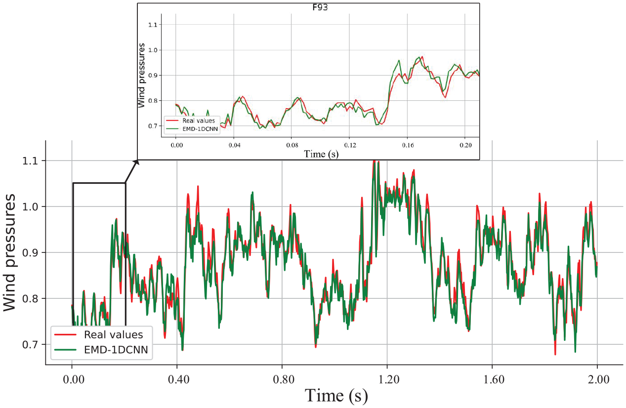
Results of prediction capabilities using the EMD-1DCNN model (F93).
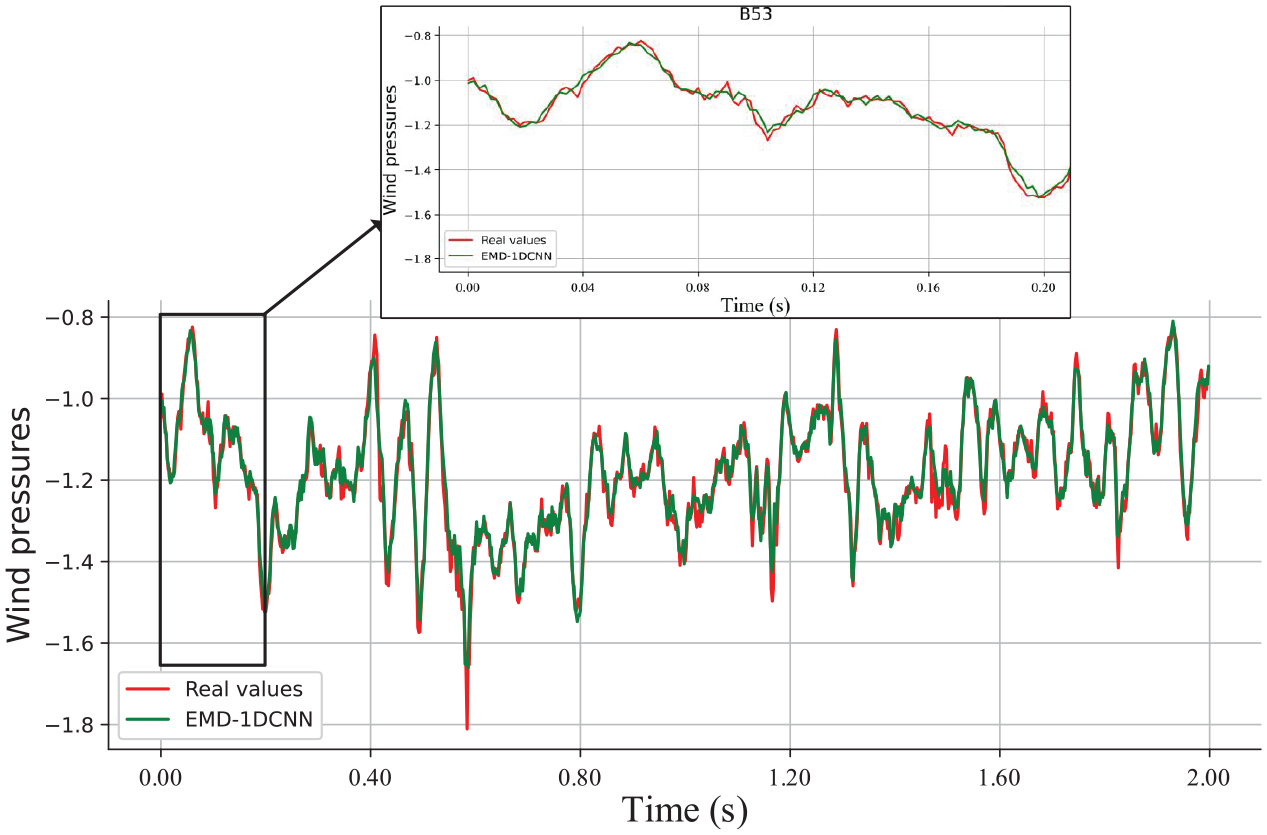
Results of prediction capabilities using the EMD-1DCNN model (B53).
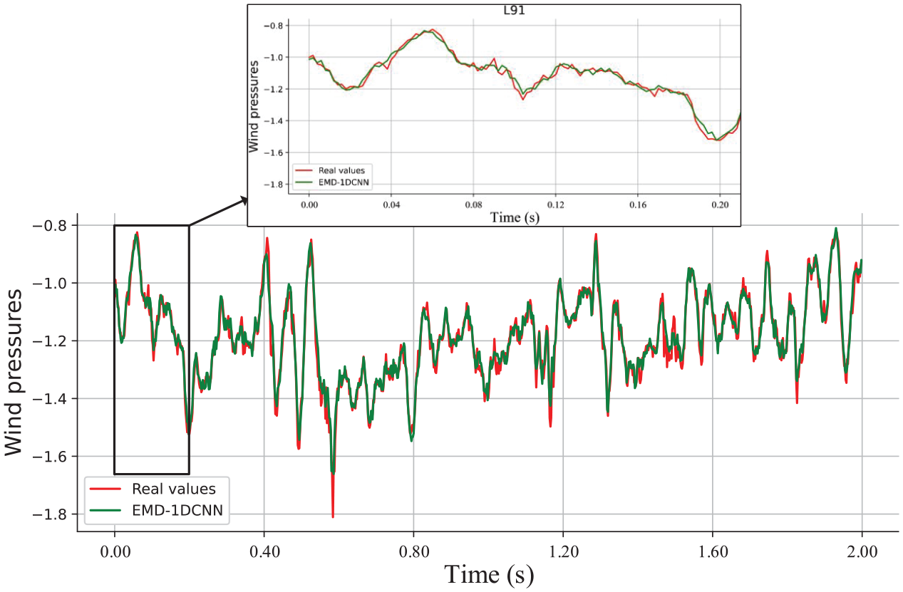
Results of prediction capabilities using the EMD-1DCNN model (L91).
In Figure 24, the bar charts represent the results of the evaluation criteria for different measured points, and the EMD-1DCNN model predicted values are in close agreement with actual values for all faces. Due to the values of
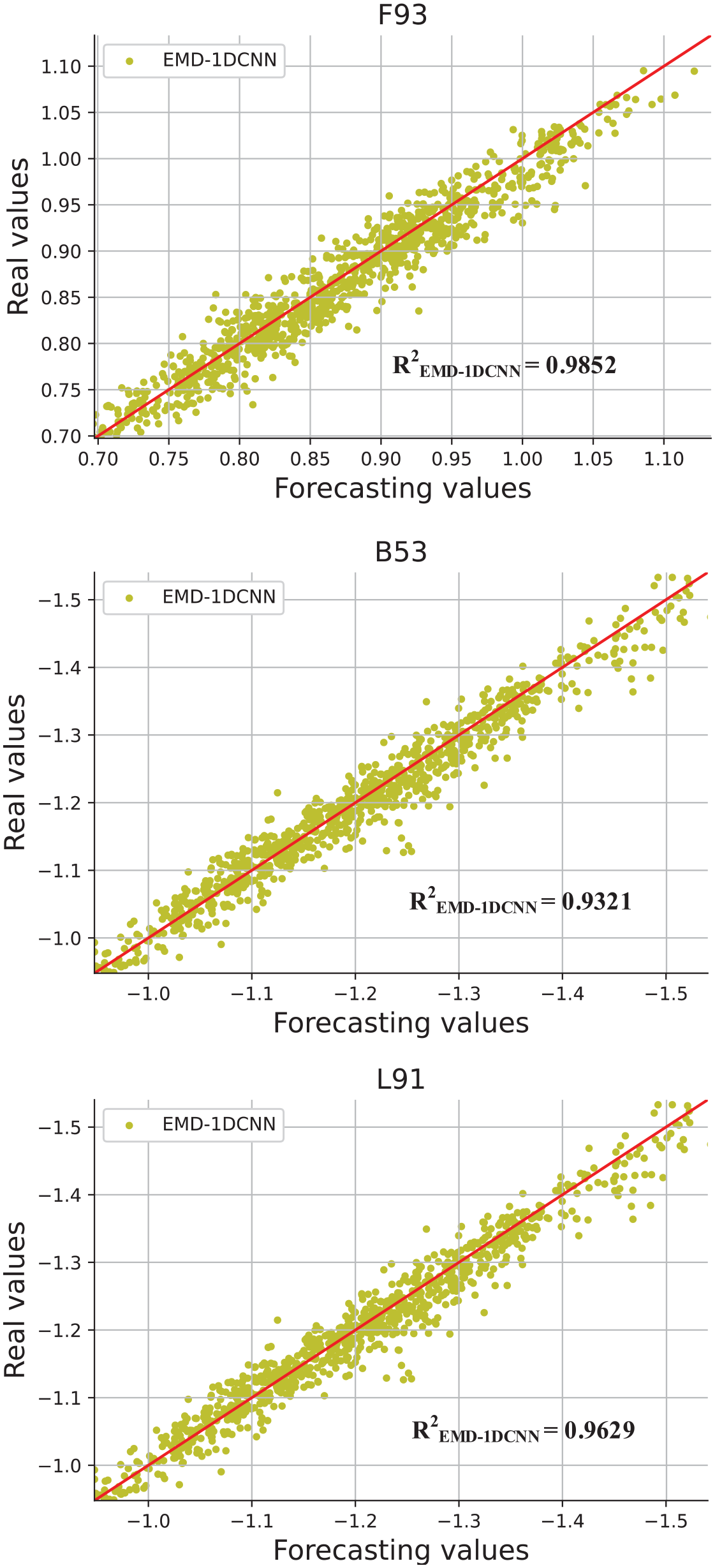
Scatter chart of different datasets (F93, B53, L91).
Effect of different portions of training data on the performance of the EMD-1DCNN model
To this end, the above EMD-1DCNN model is trained based on 50% obtained data (the first 50 s). Under this condition, the EMD-1DCNN model presents an excellent performance in predicting long-term wind pressures. In general, an increasing amount of data used in the EMD-1DCNN model can enhance the performance in predicting wind pressures. However, the EMD-1DCNN model may not have sufficient data used for training, and the effect of data length on the accuracy of prediction becomes important. To investigate the effect of different portions of training data on the performance of the EMD-1DCNN model, 0.025%–90% of the whole datasets are trained for the EMD-1DCNN model, and the remaining data are used as testing datasets. The evaluation results, including MSE, RMSE, MAE, and R-square values of F95, B11, and L91, are presented in Figures 25 to 27.
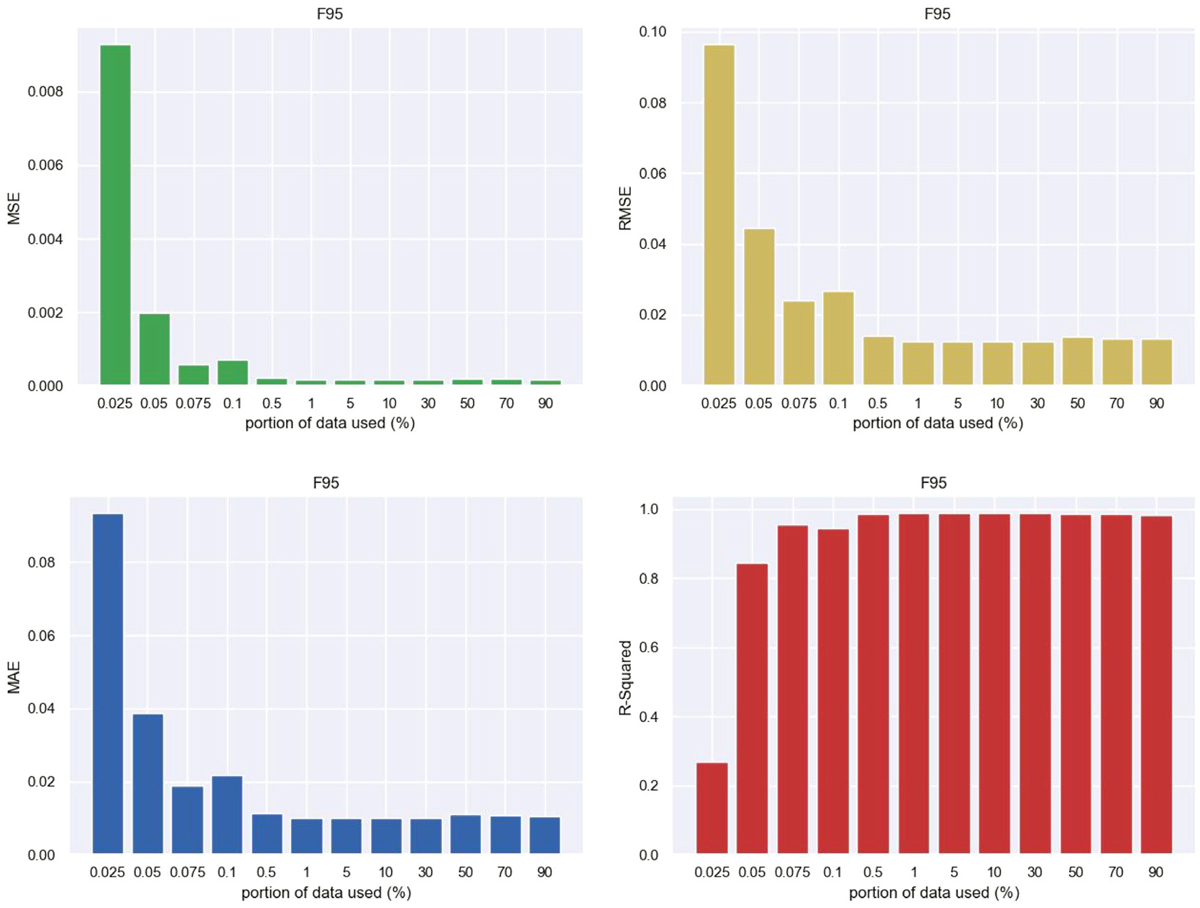
Evaluation criteria against the portion of training dataset used in the EMD-1DCNN model (F95).
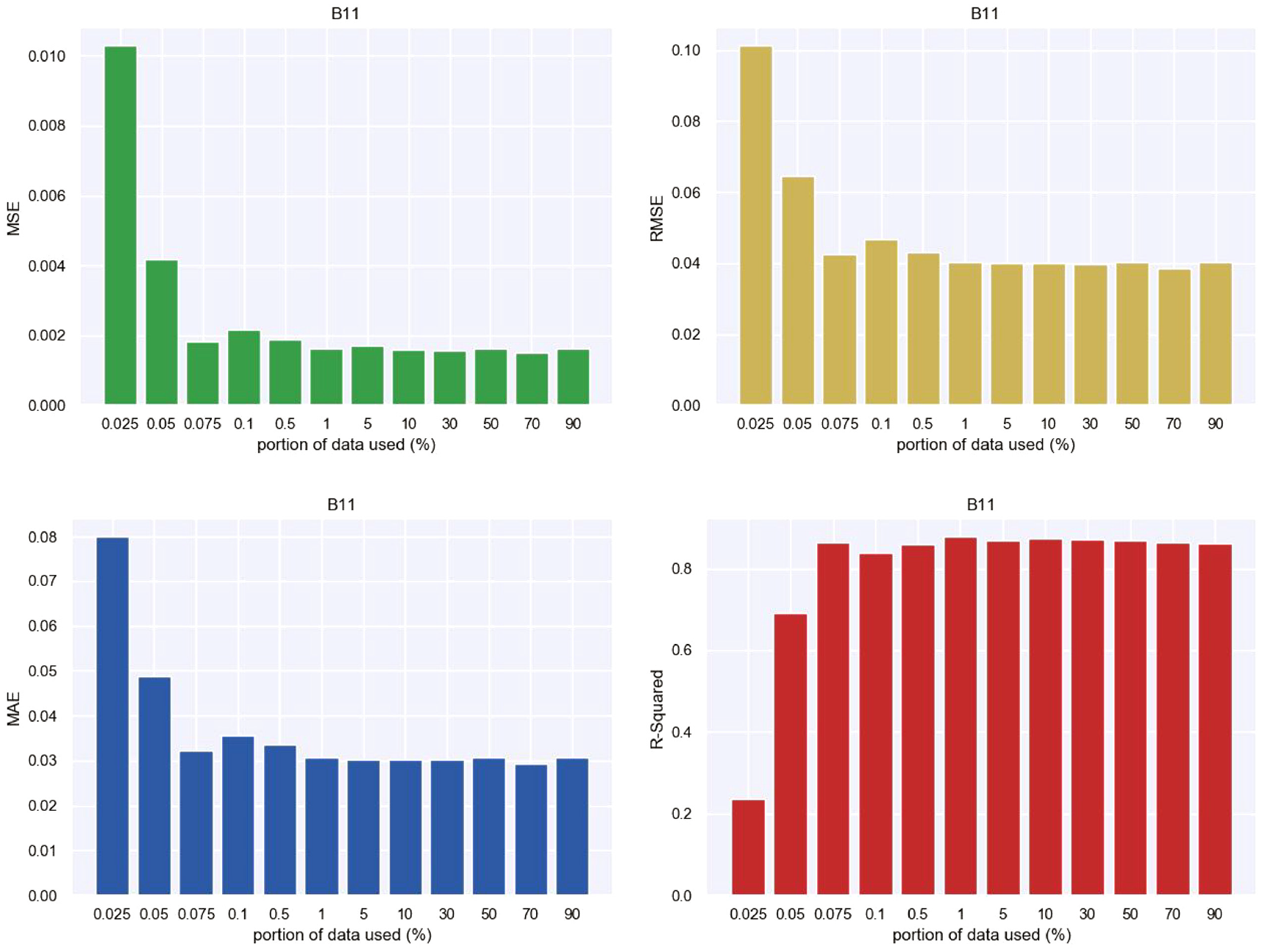
Evaluation criteria against the portion of training dataset used in the EMD-1DCNN model (B11).
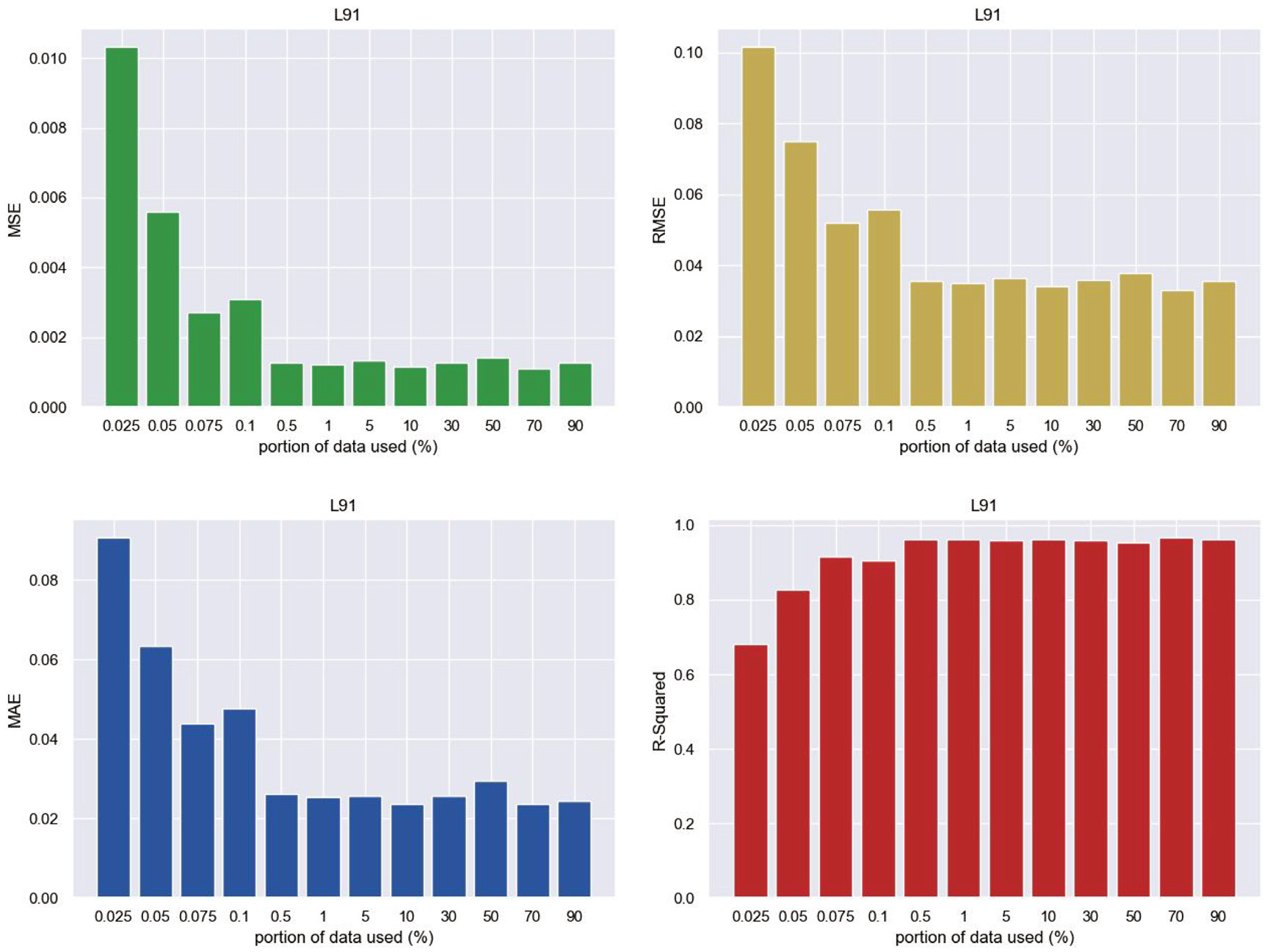
Evaluation criteria against the portion of training dataset used in the EMD-1DCNN model (L91).
It is observed from Figures 25 to 27 that when the portion of training datasets is less than 1%, the performance capability of the 1DCNN model increases with the portion of training dataset. By contrast, when the portion is larger than 1%, the performance is remarkably close as MSE, RMSE, MAE, and R-square values are close. It suggests that the EMD-1DCNN model has a good performance in predicting long-term wind pressures when the potion of a training dataset is larger than 1%, and at least 1% dataset is therefore recommended for similar predictions. When wind pressure sensors take off in an SMPSS experiment, the missing data can be predicted using the EMD-1DCNN model as long as 1% data (around 500 samples in the present study) is acquired before the pressure sensors are broken. More importantly, 1% training proportion is 500 samples, and the collection time is about 1 s in term of the sampling frequency of 500 Hz in an SMPSS experiment.
Concluding remarks
This study has predicted single wind pressures, short-term wind pressures, and long-term wind pressures on a test model for an SMPSS wind tunnel test using deep learning models, including DNN, LSTM, and EMD-1DCNN models. The main findings of the present study are summarized as follows.
(1) Both the used DNN and LSTM models present a good performance in the single predictions of wind pressures. The proposed EMD-1DCNN model is better than the DNN and LSTM models.
(2) In term of short-term data missing, the MSE, RMSE, MAE metrics of the EMD-1DCNN model are smaller than the DNN and LSTM model with the increasing number of prediction points (B53, F95, L11), which indicate that our proposed method is powerful in predicting short-term wind pressures.
(3) The EMD-1DCNN model extracts the spatial feature of wind pressure sensors and surrounding sensors to predict long-term wind pressures, and the R-square values of EMD-1DCNN are greater than 0.8, indicating that the EMD-1DCNN model has an outstanding performance in predicting long-term wind pressures.
(4) When the proportion of a training dataset is larger than 1% of the whole dataset (500 samples), the efficiency of the EMD-1DCNN model in predicting long-term wind pressures is approximately 90%. Therefore, the missing data can be well evaluated using the EMD-1DCNN model as long as 1% data (500 samples) is acquired before the pressure sensors are broken.
(5) One of limitation of this work is that EMD-1DCNN is tested using the raw wind pressure data without considering the effects of noise. Moreover, Another future research direction is to consider that the leading and tailing data make a impact on our proposed method. In particular, the extension of EMD-CNN to tackle missing value of wind pressure should be studied in the future.
Footnotes
Appendix
Four statistical indicators, including mean, standard, max, and min, are used to describe the data characteristics.
The EMD-1DCNN model performs long-term prediction for some wind pressure sensors located at the windward, lateral and backward faces of the test model.
Acknowledgements
The authors appreciate the use of the testing facility, as well as the technical assistance provided by the CLP Power Wind/Wave Tunnel Facility at the Hong Kong University of Science and Technology. The authors would also like to express our sincere thanks to the Design and Manufacturing Services Facility (Electrical and Mechanical Fabrication Unit) of the Hong Kong University of Science and Technology for their help in manufacturing the test rig of the forced vibration wind tunnel test system.
Declaration of conflicting interests
The author(s) declared no potential conflicts of interest with respect to the research, authorship, and/or publication of this article.
Funding
The author(s) disclosed receipt of the following financial support for the research, authorship, and/or publication of this article: The work described in this paper was supported by the Fundamental Research Funds for the Central Universities of China (2021CDJQY-001), the National Natural Science Foundation of China (Grant No.: 51908090), the Natural Science Foundation of Chongqing, China (Grant No.: cstc2019jcyj-msxmX0565, cstc2020jcyj-msxmX0921), the Key project of Technological Innovation and Application Development in Chongqing (Grant No.: cstc2019jscx-gksbX0017), and the National Research Foundation of Korea (NRF) grant funded by the Korea government (MSIT) (No. 2019R1G1A1095215 and 2019H1D3A1A01101442).