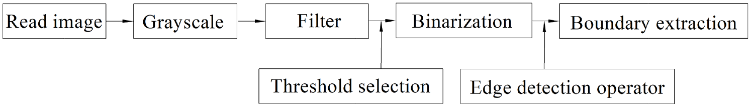
Sage Journals: Discover world-class research

Abstract

Aiming at the problems of low efficiency of the traditional method for detecting smooth plug gauges and poor repeat accuracy of measurement parameters, a measuring system for the diameter of a smooth plug gauge based on machine vision technology is designed. This system drives the work-piece to move by two-dimensional work platform and collects image data through CCD, and the diameter parameters of the smooth plug gauge are obtained by processing the image which uses the threshold neighborhood location and segmentation method. In this paper, the mechanical structure and control structure of the measuring system are designed, the measurement principle and calibration method are explained, the relationship between the diaphragm and the threshold value under a fixed light intensity, and the relationship between the light intensity and the threshold value under a fixed diaphragm are studied. Finally, experiments have verified that the measuring system can complete the measurement efficiently, automatically, and with high precision within 20 s, and the repeatability of the measurement does not exceed 1 μm.

Keywords

Smooth plug gauge the threshold neighborhood outer diameter the diaphragm the light intensity

Introduction

The measurement of hole parts is one of the important contents in the machinery manufacturing industry. In mass manufacturing industries such as automobiles and aerospace, high precision and high efficiency requirements are put forward for the inspection of hole parts. In production practice, the inspection of hole parts is widely used for measuring with smooth limit gauges. However, due to frequent use, the smooth limit gauge wears quickly, and it is necessary to be frequently measured to ensure that its own dimensions are qualified.¹

In recent years, the measurement technology based on machine vision has developed rapidly. It has become more and more widespread to use machine vision instead of human vision to engage in various industrial detection, target tracking, and other activities instead of human vision.^2–4 Photoelectric detection technology is an advanced detection technology in the field of measurement technology.^5–7 Especially in Japan, Germany, and the United States, due to the constant emphasis on the development of optical applications, some achievements have been obtained in the development of related measuring system. For example, Japan’s Kyoto Industry Group has developed ST-370 series laser displacement meters, and its measurement accuracy reaches ±0.0075 mm. The measurement accuracy of the DLG series external measuring system produced by German company reaches ±0.3 μm. The measurement accuracy of American Auto-B3 series measuring system reaches ±0.1 μm.⁸

In many measuring systems which used the machine vision technology, it measures accurate data by acquiring the overall image which has high requirements on the performance of the imaging equipment and poor economy.^9–11 A kind of image measuring instrument is studied in this paper. It only needs to calibrate the system once to achieve long-term measurement, and there is no human error, and it has very low requirements for the operator. It can realize automatic measurement with one key. It is not only economical but also high efficiency.

In this paper, a new measurement method is proposed, which is different from traditional optical measurement and the measurement which used the overall image. It takes high-precision images of part of the profile of the work-piece, which is obtained through multiple acquisitions. The image segmentation uses the threshold neighborhood location and segmentation method. In addition, combining the reading data of the raster ruler, the outer diameter of the plug gauge is measured. This method has no human error, good repeatability, and high accuracy that can reach 1μm.

System composition

Mechanical structure design

There are many structural designs of outer diameter measuring systems, Gao et al.¹² designed the system for diameter measurement, which applied structural design of infinity optical objective. The design of the measuring system in this paper includes structures such as raster ruler and surface light source. The overall design of the mechanical system is shown in Figure 1. It mainly includes the support 9, the pedestal 11, the X workbench 12 which moves perpendicular to the paper, the Y workbench 15 which moves parallel to the paper, the linear guides 8 and 14, the arc guide 5, the seat of cone 16, the upright 17, the locking device 4, the CCD camera 2, the handle 1, and other components. The mechanical structure is mainly used to provide support and location for the photoelectric system and the work-piece be measured.

Figure 1.

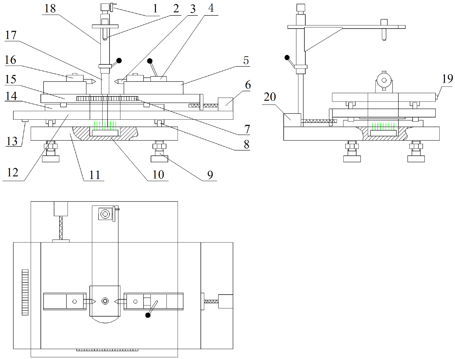
Schematic diagram of the mechanical structure of the measuring system.

The boundary of the plug gauge is one of the objects of study. In order to obtain a more accurate plug gauge boundary image, the local boundary image of the plug gauge is obtained with the same camera resolution. Therefore, the system uses a two-dimensional stage with two stepper motors and raster rulers to measure the diameter of plug gauge.

Control system design

The control part of the smooth plug gauge outer diameter measuring system includes the raster and its subdivision box, the stepper motor and its motor drive, the digital microscope and its data bus, the light source and its power supply, etc. Its control system block diagram is shown as in Figure 2.

Figure 2.

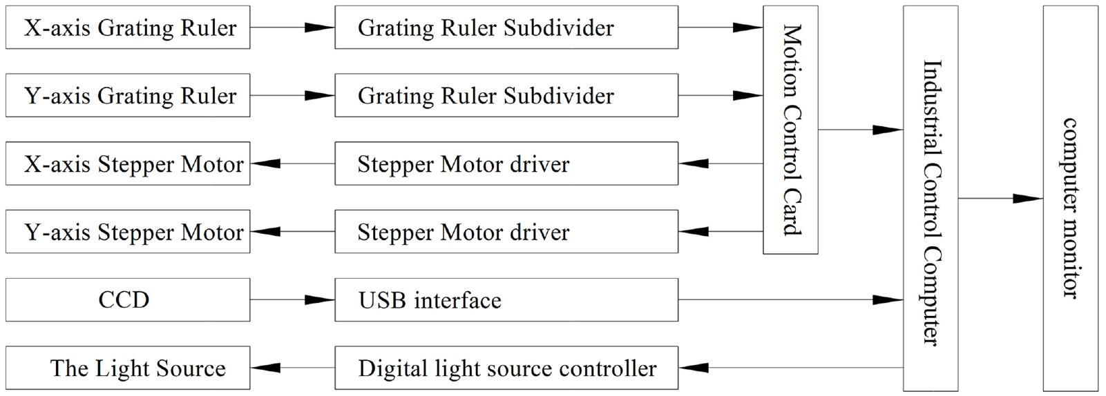
The control system block diagram.

Motion control scheme

The smooth plug gauge outer diameter measuring system adopts the two-dimensional photoelectric measurement. The X workbench and Y workbench are driven by a driving device composed of a stepping motor and a ball screw, but the location is positioned by raster and raster signal processor. The digital microscope is positioned by a upright, a guide tube, and a set of worm gears. In order to maintain the work-piece perpendicular to the axis of camera, a three-coordinate measuring instrument is used to measure and grind the contact surface is polished when the upright is installed.

Before the measurement process, the length l of the working face of the work-piece to be measured and the general diameter d of the work-piece to be measured must be input, because they are used when the origin of the image coordinate system is determined in the program.

During the measurement process, the CCD takes pictures of n transverse points on one side of the work-piece, and the movement of this process is controlled by X-axis raster ruler, X-axis stepper motor and software. In order to obtain images of n points on the other side, the Y-axis stepper motor controlled by the Y-axis raster ruler and software is used to move to the other side of the work-piece. Through these steps, the motion control of the measurement is completed. As shown in Figure 3, processes 1, 2, and 3 constitute the entire measurement motion control process.

Figure 3.

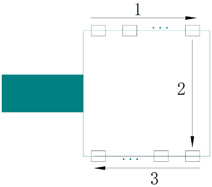
The entire measurement motion control process.

Measuring principle

There are many methods to measure the outer diameter. Liu et al.¹³ proposed a new measurement method for a tube’s endpoints based on machine vision. Hsu et al.¹⁴ propose a quadratic transformation method used to describe the relationship between the image coordinates and the world coordinates. The measuring system in this paper also involves the X-Y and U-V coordinate systems.

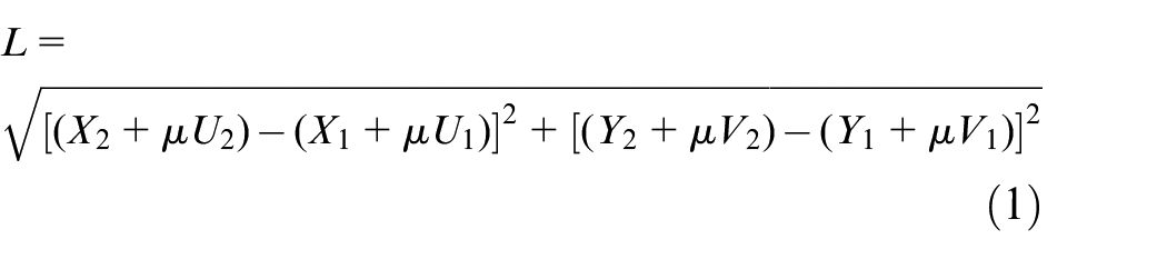
The main feature of the smooth plug gauge outer diameter measuring system is that the system involves the use of two coordinate systems, which are the orthogonal raster coordinate system X-Y formed by the X-axis and Y-axis raster rulers and the image coordinate system U-V of the image measuring system. The raster coordinate system X-Y whose unit adopts the length unit system commonly used in engineering measurement is defined as an absolute coordinate system and the image coordinate system U-V, as shown in Figure 4, whose position of the image coordinate system relative to the raster coordinate system can be changed as a relative coordinate system. The two axes of the image coordinate system should be parallel to the two axes of the raster coordinate system. The next step is equivalent calculation. The image obtained by the image measuring system is in pixels, so the measurement unit of an image with a size of m × n should be converted into that in the raster coordinate system, based on the area i × i of each photoelectric conversion element and the magnification k of the optical lens, then the equivalent conversion coefficient is obtained as μ = i/k. In this way, the conversion factor of the equivalent calculation is obtained. When the work-piece is placed between the light source and the microscope, the part hidden by the work-piece in the image is black, otherwise is white. The edge of the work-piece forms a gray transition zone due to light diffraction and other reasons, and it increases the difficulty of work-piece detection. But through a large number of experiments, the gray threshold β at which the work-piece is accurately measured can be obtained. When being measured, the edge of the work-piece may not be parallel to the axis of the coordinate system. The measuring system obtains the images of the detection points a and b on the work-piece c, and extracts the edge of the image with the gray threshold β. The origin coordinates of the image coordinate system can be obtained from the raster ruler which are (X₁, Y₁) and (X₂, Y₂). Therefore, the coordinates of point a and point b are (X₁ + μU₁, Y₁ + μV₁) and (X₂ + μU₂, Y₂ + μV₂). Then, the dimension L between the two points a and b can be calculated according to the following formula (1):

\begin{matrix} L = \\ \sqrt{{[(X_{2} + μ U_{2}) - (X_{1} + μ U_{1})]}^{2} + {[(Y_{2} + μ V_{2}) - (Y_{1} + μ V_{1})]}^{2}} \end{matrix}

(1)

Figure 4.

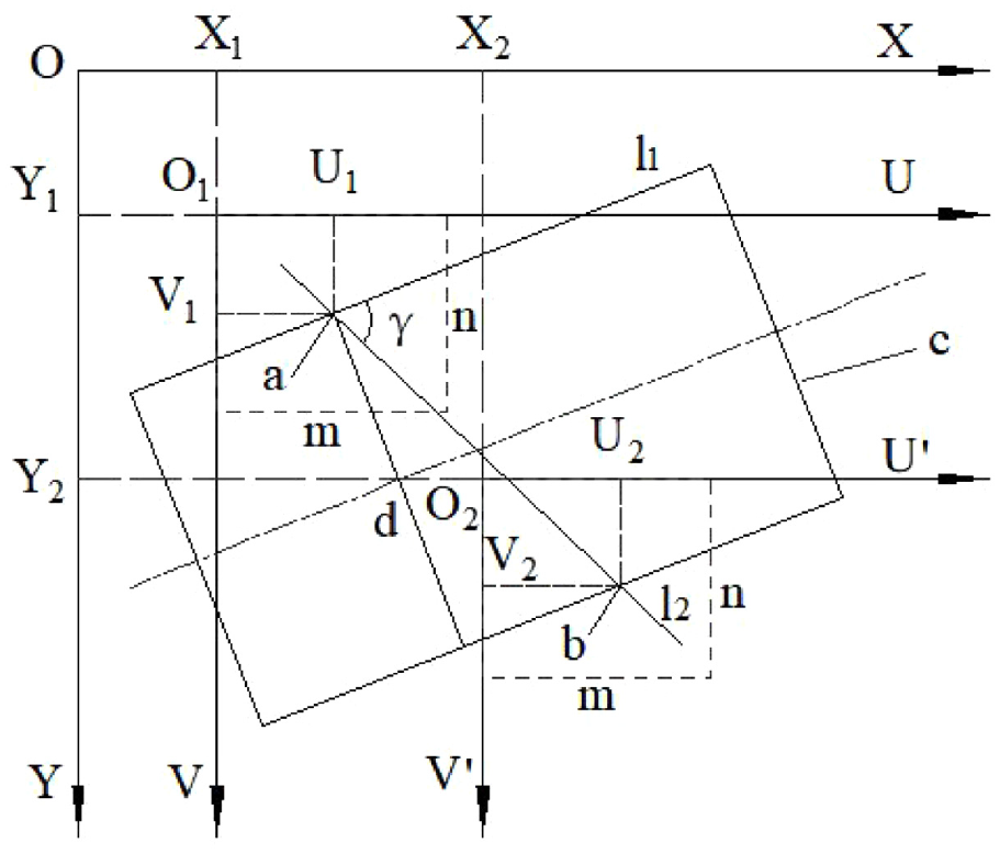
The measurement principle diagram.

The image edge line l1 and the edge line l2 can also be obtained through the slopes of the two points a and b. Assuming that they are K₁ and K₂, the angle γ can be calculated according to the following formula (2):

\tan γ = | (K_{1} - K_{2}) / (1 + K_{1} K_{2}) |

(2)

Then, the diameter d of smooth plug gauge can be calculated according to the following formula:

d = L \sin γ

The measuring system adopts advanced measurement principles which can effectively avoid errors caused by non-parallelism between the edge of the work-piece and the image coordinate system.

The principle of CCD calibration and calibration process

The CCD calibration is a very critical part, and Xiong et al.¹⁵ propose a method to calibrate the CCD in the frequency domain. Ma et al.¹⁶ presente a line-scan camera calibration method in a plane not perpendicular to but parallel to the optical axis, without requiring the camera motion or a complex calibration pattern. Peng et al.¹⁷present a precise calibration method for a CCD with a small field of view. In the design of this paper, CCD calibration is based on raster ruler and resolution.

The calibration of the pixel size of the digital microscope is carried out by using a standard rod with diameter D. The standard rod is clamped on the measuring system. According to the image on the computer display, the height of the guide tube and the position of the CCD should be adjusted and changed until the edge of the standard rod is clear. The edge of the standard rod is moved to the middle of the image coordinate system, and the edge state characteristics and the position of the raster coordinate system are recorded. The transition zone threshold at this time is used as the segmentation threshold to extract the edge of the image, and the curve equation of the edge is obtained by fitting. Then the X direction is kept unchanged, and the standard rod is moved to the other side along the Y direction. When the edge state feature is basically the same as the previous one, the coordinate position of the raster coordinate system is recorded. The edge of the image at this time is extracted by using the previous transition zone threshold, and the curve equation of the edge is obtained by fitting. According to the reading of the raster and the resolution of the digital microscope, the actual size of the pixel in the current state can be calibrated.

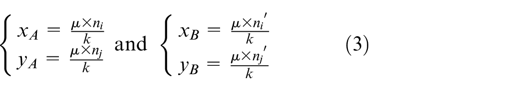
A standard rod with a diameter of D is used as a debugging part. Figure 5 shows a schematic diagram of the calibration process. The magnification k of the optical lens is adjusted, and the digital image of edge is represented by a 14 × 10 square grid. When the image coordinate system is XOY, the reading D₁ of the raster is read and recorded. The digital image at point A is acquired and threshold-ed. Then the image coordinate system is moved to the other side X′O′Y′ of the standard rod, the reading D₂ of the raster is read and recorded. The digital image at point B is acquired and thresholded. Therefore, the reading difference of the raster is n′ = D₂ − D₁. Because the resolution of the digital microscope is m×n, the pixel position of point A in the digital image is calculated, assuming it is (n_i, n_j). Similarly, B is (n_i′, n_j′). It is known that the actual length l′ of the raster ruler and the raster ruler is subdivided into N divisions. Then, the actual distance of each division of the raster is l′/N. The position of A in the image is represented by (x_A, y_A), the pixel size is represented by μ, and the number of rows and columns of A and B in the digital image are represented by n_i, n_j, n_i′, n_j′. Then the coordinates (x_A, y_A) and (x_B, y_B) are:

{\begin{matrix} x_{A} = \frac{μ \times n_{i}}{k} \\ y_{A} = \frac{μ \times n_{j}}{k} \end{matrix} and {\begin{matrix} x_{B} = \frac{μ \times {n_{i}}^{'}}{k} \\ y_{B} = \frac{μ \times {n_{j}}^{'}}{k} \end{matrix}

(3)

Figure 5.

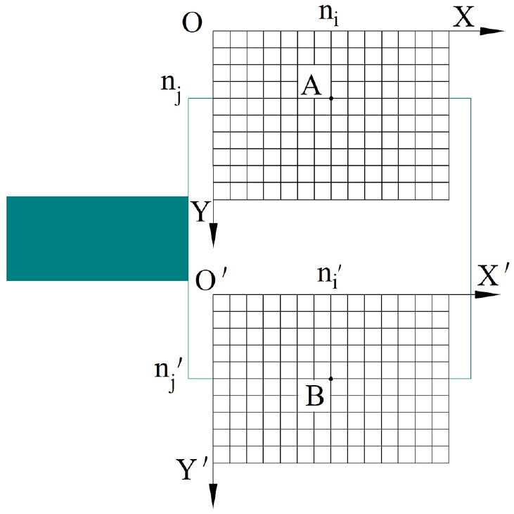
The schematic diagram of the calibration process.

According to the calculation formula (3), the calculation formula for the diameter D of the standard rod can be deduced. Furthermore, the calculation formula (4) for the pixel size μ can be deduced too. It is:

\begin{matrix} D = (D_{2} - D_{1}) (l^{'} / N) - \frac{(n - {n_{j}}^{'}) μ}{k} + \frac{(n - n_{j}) μ}{k} \\ μ = \frac{D - (D_{2} - D_{1}) (l^{'} / N)}{{n_{j}}^{'} - n_{j}} k \end{matrix}

(4)

Image processing

Image processing and acquisition of plug gauge boundaries

The process of digital image processing is shown in Figure 6.

Figure 6.

The general process of digital image processing.

As shown in the Figure 3, the motion control scheme consists of three processes. The images obtained in process 1 are processed to form one boundary of the plug gauge and the images obtained in process 3 are processed to form the other boundary of the plug gauge, as shown in Figure 7.

Figure 7.

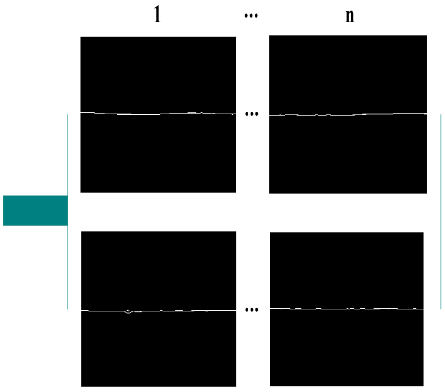
The composition of the plug gauge boundary.

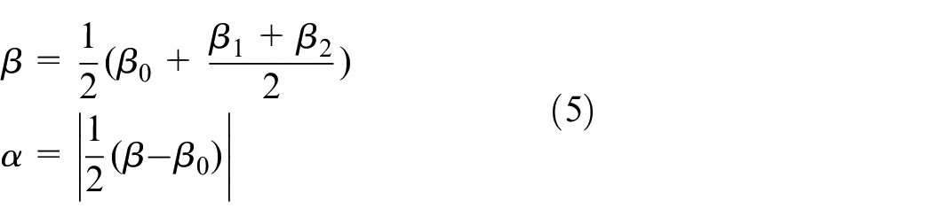
Image threshold neighborhood location and segmentation method

The image segmentation of the measuring system uses the threshold neighborhood location and segmentation method. Because the resolution of the image acquired by the image sensor is m × n, the image is stored in the computer in the form of a two-dimensional matrix with m rows and n columns. Therefore, there are m grayscale values in each column of the matrix and n grayscale values in each row. Image segmentation is also based on this two-dimensional matrix. A threshold β and a neighborhood radius α are selected, so the neighborhood of the threshold is (β − α, β + α). The average grayscale value of the overall image is selected as the initial threshold β₀. The image is segmented into two parts by the initial threshold. The average grayscale value of each part are calculated as β₁ and β₂. Then the threshold β and the neighborhood radius α are:

\begin{matrix} β = \frac{1}{2} (β_{0} + \frac{β_{1} + β_{2}}{2}) \\ α = | \frac{1}{2} (β - β_{0}) | \end{matrix}

(5)

A two-dimensional array Z(x, y) is used to store data. Its x is used to store the number of columns, and y is used to store the average value of all gray levels in the threshold neighborhood of each column. If all the grayscale values of a column are not in the neighborhood of the threshold, then y is −1. Each column is validated from left to right, and the points whose y value is −1 are deleted. Finally, a two-dimensional array is obtained, and the value in it is the grayscale value of the real edge, as shown in Figure 8.

Figure 8.

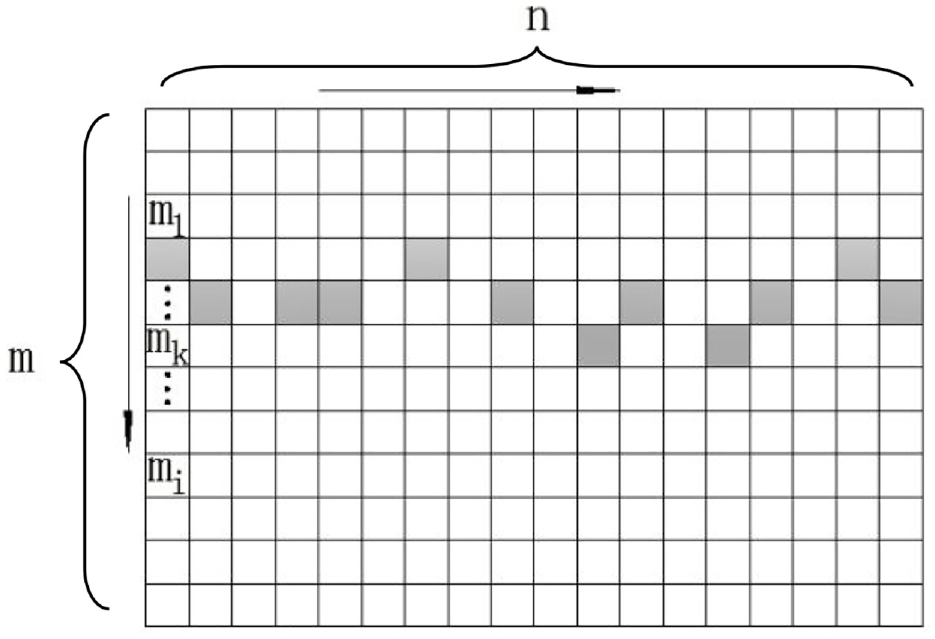
Threshold neighborhood location and segmentation method.

The value of x in the two-dimensional array Z is used as the ordinate and the value of Y is used as the abscissa. The straight line is obtained by the least squares method and the slope of the edge straight line is obtained, which will be used in the calculation of the measurement results later.

As shown in Figure 7, after the acquired images are processed according to the above method, the pictures obtained in process 1 and 3 are sequentially placed on a horizontal plane. Because of the gap between the guide rail and the slider, the workbench will have uncertain offset in the process of movement. It will be found that the plug gauge boundary of each picture is not on a horizontal line. In order to obtain the entire boundary of the plug gauge, p_n points are evenly selected on the boundary of each segment. As shown in Figure 9, the straight line L is obtained by using the least squares method to fit all n × p_n points, and it is one boundary of the plug gauge. In the same way, the other side boundary of the plug gauge can be obtained, and the diameter of the plug gauge can be obtained by using the measurement principle shown in Figure 3.

Figure 9.

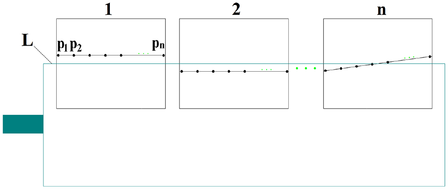
The schematic diagram of the contour acquisition process.

The relationship between threshold and diaphragm

In the measuring system, a surface light source is used. Bernard et al.¹⁸study the relationship between filters and light sources, etc. Bruehl et al.¹⁹ discuss the existence of control holes and slits. In order to minimize the impact of non-parallel light on the edge image of the work-piece, a diaphragm is installed between the work-piece and the light source, as shown in Figure 10.

Figure 10.

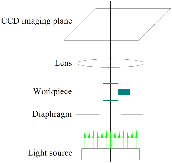
The position of diaphragm.

Therefore, it is necessary to find the relationship between the threshold value and the diaphragm width during image segmentation under a fixed light intensity. The experiment was carried out under the conditions of light intensity of 160, temperature of 21°C, and humidity of 42%. The relationship between the threshold and the width of the diaphragm during image segmentation was found through the experiments. Taking the measurement data of a 30 mm diameter smooth plug gauge as an example, and the accurate value of its outer diameter measured by thread measuring machine (XPL-C200, IAC, NLD) is 30.00465 mm.

Before the measurement, high-strength alcohol was used for cleaning the surface of the plug gauge and a marble temperature table was used to set the temperature of it in the metrology laboratory. The measured data is shown in Table 1.

Table 1.

Data of diaphragm and threshold for a smooth plug gauge with the diameter of 30 mm.

Diaphragm (mm)	Smooth plug gauge outer diameter measuring system
Diaphragm (mm)	Threshold	First measured value (mm)	Second measurement value (mm)	Third measurement value (mm)
5	60	30.00455	30.00457	30.00459
5	60	30.00484	30.00487	30.00488
6	62	30.00475	30.00459	30.00443
6	62	30.00489	30.00473	30.00458
7	96	30.00466	30.00460	30.00451
7	96	30.00479	30.00474	30.00463
8	94	30.00450	30.00472	30.00471
9	126	30.00457	30.0047	30.00465
10	131	30.00454	30.00475	30.00454
10	131	30.00460	30.00480	30.00460

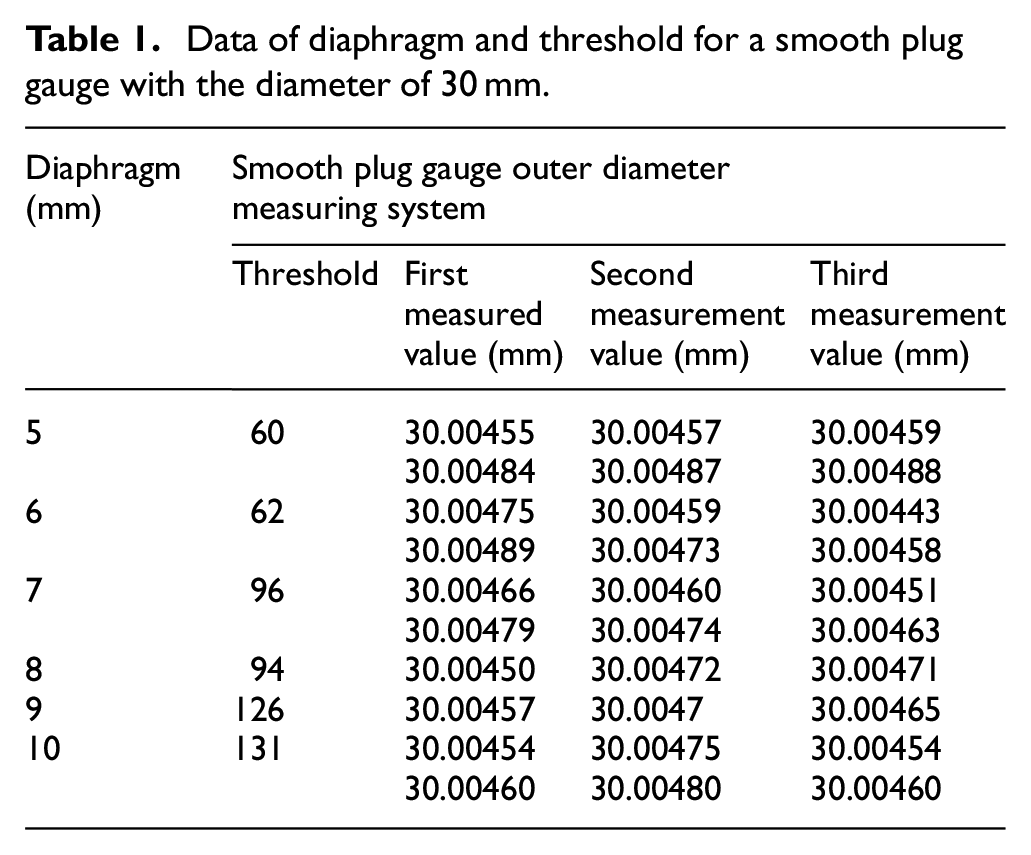
The data in the table need attention. For example, when the diaphragm width is 7 mm and the threshold value is 63, the outer diameter measurement value is slightly smaller than the accurate value; when the threshold value is 64, the measurement value is slightly larger. The boundary of the plug gauge is extracted respectively at the thresholds 63 and 64, then their intermediate value is taken as the boundary data for the final measurement calculation. To represent this situation, a non-integer threshold is used.

The relationship between the threshold value and the diaphragm width is displayed as a smooth curve, as shown in Figure 11, it contains smooth plug gauges with a diameter of 3, 10, 20, 30, 40, and 50 mm.

Figure 11.

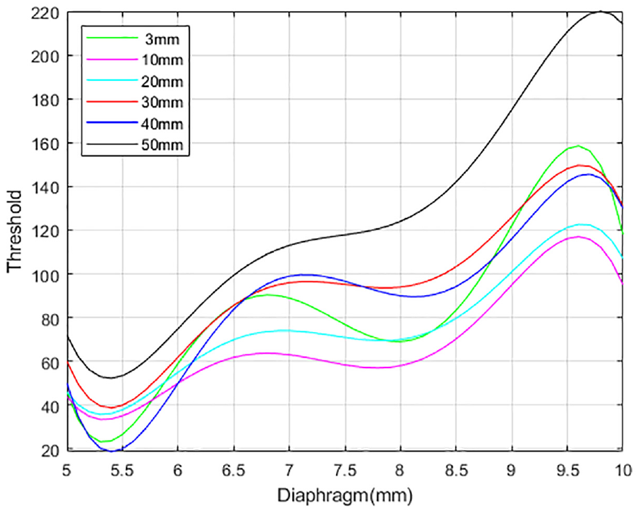
The relationship between threshold and diaphragms.

The relationship between threshold and light intensity

As shown in Figure 12, the experiment of threshold and light intensity is used to illustrate the clarity of the boundary at different light intensities. In algorithm, Baigvand et al.²⁰ compared the feature values with the threshold values which are predetermined by an expert. In this paper, because that the light intensity is less than 120 will make the image of the work-piece dark, image threshold processing can only be carried out in a very small threshold range, and a small threshold change will cause a large deviation in the grayscale value of the edge of the work-piece. The same effect will be caused when the light intensity is higher than 190. Therefore, the appropriate light intensity will reduce the difficulty of system debugging.

Figure 12.

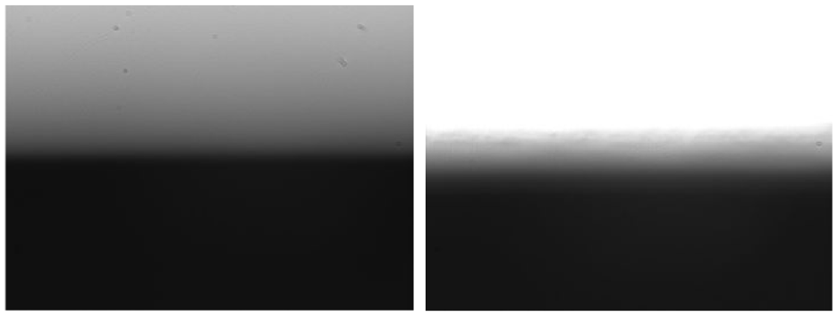
Pictures with too high or too low light intensity.

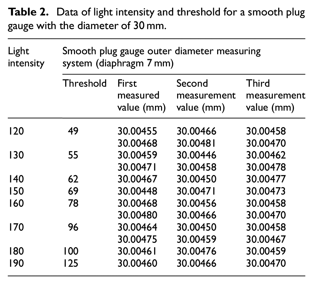
Therefore, it is necessary to find the relationship between the threshold value and the light intensity during image segmentation under the condition of a fixed diaphragm. The experiment took the diaphragm of 7 mm as an example, and was carried out at a temperature of 23°C and a humidity of 52%. The data in Table 2 is the measurement data of a 30 mm diameter smooth plug gauge, and the accurate value of its outer diameter measured by thread measuring machine (XPL-C200, IAC, NLD) is 30.00465 mm.

Table 2.

Data of light intensity and threshold for a smooth plug gauge with the diameter of 30 mm.

Light intensity	Smooth plug gauge outer diameter measuring system (diaphragm 7 mm)
Light intensity	Threshold	First measured value (mm)	Second measurement value (mm)	Third measurement value (mm)
120	49	30.00455	30.00466	30.00458
120	49	30.00468	30.00481	30.00470
130	55	30.00459	30.00446	30.00462
130	55	30.00471	30.00458	30.00478
140	62	30.00467	30.00450	30.00477
150	69	30.00448	30.00471	30.00473
160	78	30.00468	30.00456	30.00458
160	78	30.00480	30.00466	30.00470
170	96	30.00464	30.00450	30.00458
170	96	30.00475	30.00459	30.00467
180	100	30.00461	30.00476	30.00459
190	125	30.00460	30.00466	30.00470

The relationship between the threshold and light intensity is displayed as a smooth curve, as shown in Figure 13, it contains smooth plug gauges with a diameter of 3, 10, 20, 30, 40, and 50 mm.

Figure 13.

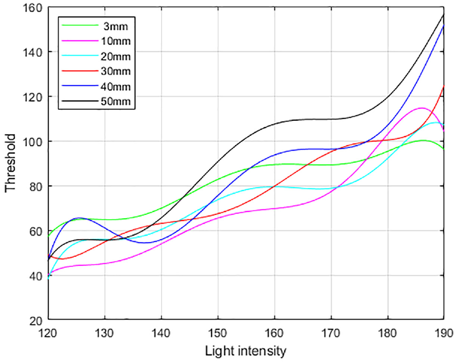
The relationship between threshold and light intensity.

Experiment and analysis

As shown in Figure 14, it is the physical image of the smooth plug gauge outer diameter measuring system.

Figure 14.

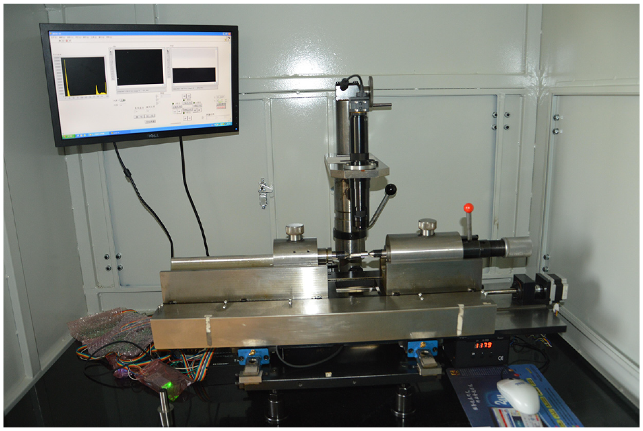
The physical picture of the measuring system.

Under the experimental conditions of room temperature of 23°C, a diaphragm of 7 mm, a light intensity of 169, and a humidity of 45%, the data of smooth plug gauges with diameter range from 1.3 to 50 mm were measured, and the exact value of their outer diameters was measured by thread measuring machine (XPL-C200, IAC, NLD).

The measurement data is shown in the Table 3.

Table 3.

Experimental results of measuring system.

Threshold	Smooth plug gauge outer diameter measuring system (diaphragm 7 mm)
Threshold	Measurements (mm)			Average value (mm)	Exact value (mm)	Difference (mm)
84	1.3021	1.3022	1.3021	1.3021	1.3020	0.0001
74	2.0018	2.0018	2.0017	2.0018	2.0019	−0.0001
121	4.0026	4.0026	4.0027	4.0026	4.0025	0.0001
74	6.0018	6.0018	6.0017	6.0018	6.0019	−0.0001
75	8.0029	8.0030	8.0029	8.0029	8.0028	0.0001
77	10.0048	10.0050	10.0049	10.0049	10.0046	0.0003
67	12.0019	12.0020	12.0019	12.0019	12.0017	0.0002
69	14.0028	14.0029	14.0028	14.0028	14.0025	0.0003
62	16.0052	16.0051	16.0050	16.0051	16.0048	0.0003
66	18.0038	18.0039	18.0038	18.0038	18.0036	0.0002
74	20.0051	20.0052	20.0051	20.0051	20.0048	0.0003
72	22.0048	22.0049	22.0048	22.0048	22.0050	−0.0002
66	24.0043	24.0046	24.0045	24.0045	24.0047	−0.0002
85	26.0035	26.0036	26.0036	26.0036	26.0031	0.0005
81	28.0053	28.0054	28.0053	28.0053	28.0049	0.0004
96	30.0048	30.0048	30.0048	30.0048	30.0046	0.0002
105	34.0064	34.0067	34.0066	34.0066	34.0064	0.0002
101	36.0050	36.0051	36.0051	36.0051	36.0053	−0.0002
95	38.0028	38.0028	38.0029	38.0028	38.0030	−0.0002
99	40.0081	40.0082	40.0082	40.0082	40.0080	0.0002
115	42.0059	42.0060	42.0060	42.0060	42.0057	0.0003
118	44.0048	44.0048	44.0048	44.0048	44.0050	−0.0002
109	46.0056	46.0055	46.0054	46.0055	46.0060	−0.0005
129	48.0044	48.0045	48.0044	48.0044	48.0042	0.0002
113	50.0081	50.0081	50.0082	50.0081	50.0083	−0.0002

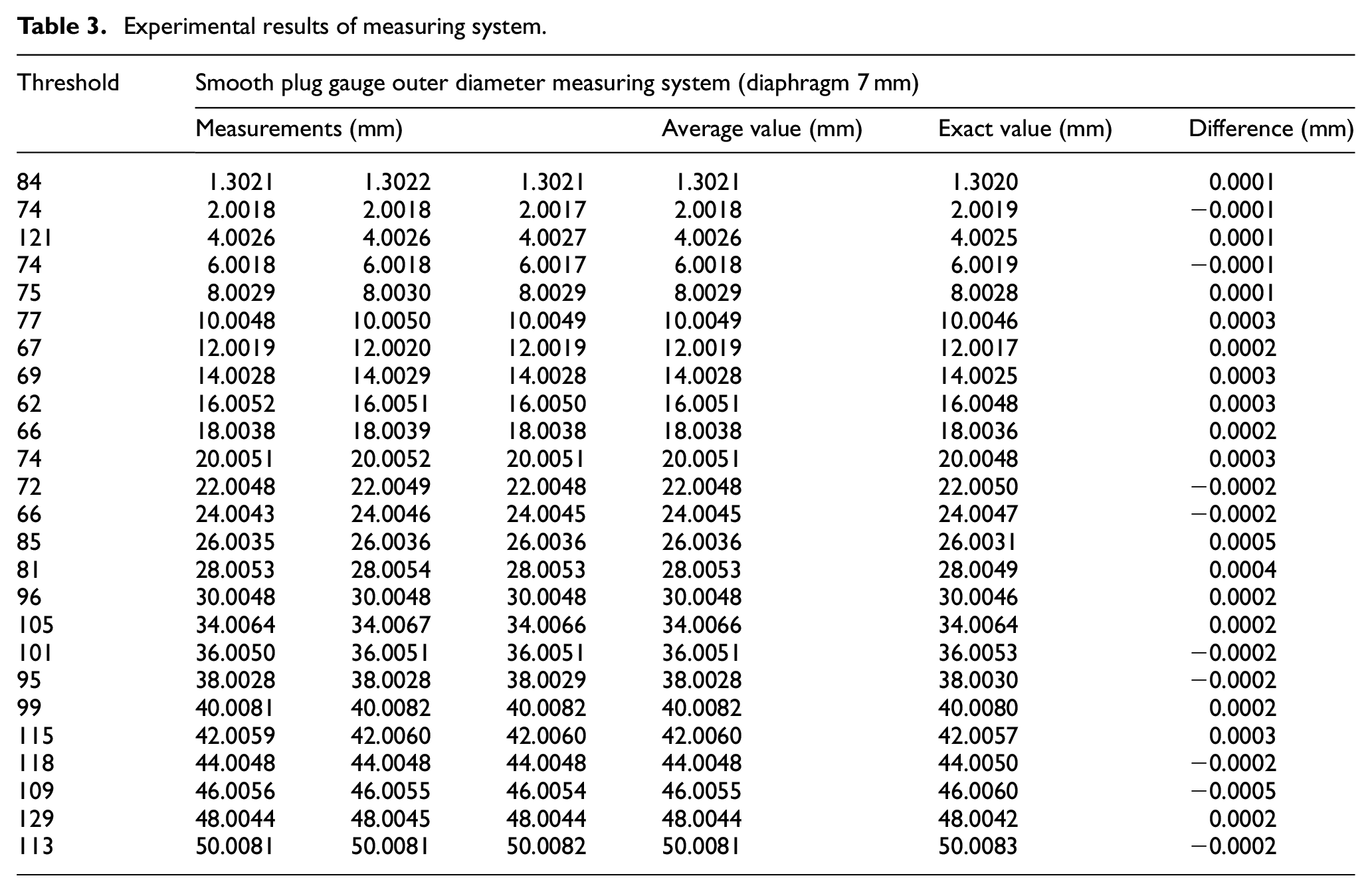
After a lot of experiments, it is found that a plug gauge of certain has a corresponding threshold that enables the plug gauge to be accurately measured.

Conclusions

In this work, a measuring system for the diameter of a smooth plug gauge based on machine vision technology was successfully developed. Different from conventional image measurement that take overall image to obtain accurate data, it takes high-precision images of part of the profile of the work-piece. The profile of the work-piece is obtained through multiple acquisitions.The image segmentation uses the threshold neighborhood location and segmentation method. In addition, the use of advanced measurement principles can effectively avoid errors caused by the non-parallelism of the work-piece edge and the image coordinate system. The system can automatically, efficiently and accurately measure the diameter parameters of a smooth plug gauge with high measurement repeatability. The relationship between the diaphragm and the threshold under the fixed light intensity and the relationship between the light intensity and the threshold under the fixed diaphragm are simultaneously studied.

Experimental results demonstrated that:

The diameter range measured by the system is 0–50 mm which is clearly proposed by the research purpose.

The measurement accuracy and repeat measurement accuracy of the system are verified, and the measurement errors are less than 1 μm.

The repeatability of the measurement does not exceed 1 μm.

Footnotes

Declaration of conflicting interests

The author(s) declared no potential conflicts of interest with respect to the research, authorship, and/or publication of this article.

Funding

The author(s) disclosed receipt of the following financial support for the research, authorship, and/or publication of this article: This work was supported by the Shaanxi Provincial Department of Education Project [Grant No. 12JK0666].

ORCID iD

Laijian Feng

References

Song

Lin

Hao

. Automatic recognition method for optical measuring instruments based on machine vision. Trans Tianjin Univ 2008; 14(3): 202–207.

Zhao

Sun

, et al. A CCD based machine vision system for real-time text detection. Front Optoelectron 2020; 13: 418–424.

Connolly

. Machine vision advances and applications. Assem Autom 2009; 29(2): 106–111.

Ranky

. Advanced machine vision systems and application examples. Sens Rev 2003; 23(3): 242–245.

Golnabi

Asadpour

. Design and application of industrial machine vision systems. Robot Comput Integr Manuf 2007; 23(6): 630–637.

Hunt

Carey

. A machine vision system for the braid angle measurement of tubular braided structures. Text Res J 2019; 89(14): 2919–2937.

Kanade

Asada

. Noncontact visual three-dimensional ranging devices. Proc SPIE 1981; 283: 48–55.

. A research of non-contact micro-displacement measurement system based on linear CCD. Changchun City, Jilin Province, China: Changchun University of Science and Technology, 2011 (in Chinese).

Chen

. Compensation of thread profile distortion in image measuring screw thread. Measurement 2018; 129: 582–588.

10.

Wang

Zhao

. Research on tooth profile deviations measurement method based on the optical image measuring instrument. Adv Mater Res 2013; 712–715: 1979–1982.

11.

Shen

Wang

Chen

. Research on screw thread form based on non-contact measurement. Appl Mech Mater 2011; 101–102: 593–596.

12.

Gao

Zhang

. High precision machine vision system for outer diameter inspection bearing. Key Eng Mater 2013; 552: 313–318.

13.

Liu

Jin

Liu

, et al. Accurate measurement method for tube’s endpoints based on machine vision. Chin J Mech Eng 2017; 30(1): 152–163.

14.

Hsu

Ngo

. Development of a faster classification system for metal parts using machine vision under different lighting environments. Int J Adv Manuf Technol 2019; 100(9–12): 3219–3235.

15.

Xiong

Xiangli

, et al. Image reconstruction method based on CCD calibration in frequency domain. Appl Opt 2015; 54(14): 4561–4565.

16.

Dong

Tian

, et al. Line-scan CCD camera calibration in 2D coordinate measurement. Optik 2014; 125(17): 4795–4798.

17.

Peng

Vienne

Han

, et al. Precise calibration of CCD images with a small field of view. Astron Astrophys 2004; 424(1): 339–344.

18.

Jiang

Shiau

MYR

. A systematic methodology for determining/optimizing a machine vision system’s capability. Mach Vision Appl 1990; 3(3): 169–182.

19.

Bruehl

. Description and industrial applications of a standard machine vision system not requiring task-specific development. Proc SPIE 1994; 2249: 408–418.

20.

Baigvand

Banakar

Minaei

, et al. Machine vision system for grading of dried figs. Comput Electron Agric 2015; 119: 158–165.

Development of a measuring system for the diameter of a smooth plug gauge based on machine vision technology