
Abstract
As we all known, estimating the proportion of passenger route choice is of great significance in almost every aspect of urban rail transit control system, including passenger allocation, fare clearing and flow control strategies. Existing researches only pay attention to the route choice through travel time, but usually ignore the influence in different periods of the day. Therefore, this paper proposes a novel estimation method for the proportion of passenger route choice in different periods. Firstly, by introducing the normalized value of passenger flow and the standard coefficient of peak passenger flow, the train operation time is divided into peak and flat periods. Secondly, the travel time distribution of each route can be obtained by estimating the expected value and standard deviation of passenger travel time in each different period. The Naïve Bayes algorithm is further employed to realize the identification of the proportion of passenger route choices. Finally, this proposed algorithm is applied to Hangzhou Metro. The result shows that by using the segmented estimation, the error can be reduced by more than 60% compared with the whole-day experiment, which indicates the superiority of the method.
Keywords
Introduction
The networked operation of urban rail transit provides passengers with diversified route choices between origin-destination (OD). However, the mode of “one ticket transfer” only requires passengers swipe their ticket cards when they enter and exit the stations. Though it brings much convenience to passengers, but makes it difficult to confirm the specific routes of passengers. Mastering the travel routes of passengers is the basic to calculate the passenger flow of urban rail transit lines and evaluate the operation level of urban rail transit. It also guides the operation management department to improve the operation organization of urban rail transit and formulate operation control strategy reasonably and scientifically.
Some scholars have made a range of achievements on passenger route choice. The early researches were mainly based on the multi-routes probability distribution method,1–6 by which the generalized travel cost of each route is obtained by establishing impedance functions including travel time, transfer time and other factors, and then the probability of route selection is calculated by LOGIT model and its deriving forms. Recently, with the emergence and wide application of automatic fare collection system, the information such as passengers’ enter stations with enter time, exit stations with exit time can be easily obtained. It provides researchers with new perspectives of passenger route choice estimation. Zhou et al. 7 analyzed the travel time elements of urban rail transit passengers in detail. This research pointed out the travel time of passengers in each path obeyed normal distribution, and gained the path selection ratio through the AFC data. Hong et al. 8 proposed an urban rail transit passenger flow distribution model, in which clustering technology was used to integrate similar travel times in AFC data and divided them into the same path. It provided a new idea for the study of passenger route selection. Cheng et al. 9 filtered the unreasonable data in AFC information and analyzed the travel time characteristics of non-transfer passengers and transfer passengers. They verified that the passengers’ travel time obeyed logarithmic normal distribution and established the model of urban rail transit passenger travel path selection. Zhang et al. 10 compared the correlation of travel time among multiple paths according to the AFC data, and established the route choice model based on the Gaussian mixture model. Ni et al. 11 studied the passenger path choice problem of multi-track rail transit network, and fitted the parameters of the established path selection model according to the AFC data. All of the above studies are considered from the perspective of aggregate rather than the individual passengers, ignoring the differences among passengers.
Wang et al. 12 used AFC data to identify the passengers’ travel information to speculate the travel chain of individual passengers. The results were corrected by the physical relationship between lines. Hu et al. 13 calculated the travel time parameters of a single passenger with AFC data, and considered the matching relationship between train schedules to determine the passenger route selection scheme. Wu et al. 14 mined AFC data in Beijing and adopted the similarity measurement method to match individual travel time with travel routes. The proportion of travel route choice was obtained by integrating individual data. Sun et al. 15 restored multiple travel chains of passengers according to AFC data and train schedule. The probability of each travel chain was calculated according to departure time and the chain with the highest probability was selected as the passenger route option.
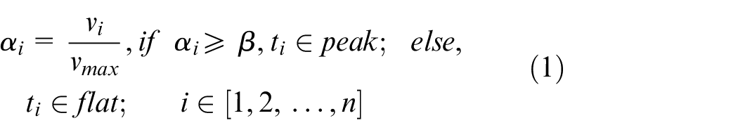
However, the previous studies mainly focus on the total travel time of passengers, and rarely take into account the change of travel time distribution of passengers at different periods. Some studies have shown that 16 the route choice characteristics of passengers is varying throughout a day. The study results will be biased without the consideration of these. Therefore, this paper proposes an approach to estimate the proportion of passenger route choice for urban rail transit control system with the consideration of different periods. The train operation time is divided into different stages with the granularity of τ, and then the normalized value of passenger flow corresponding to each stage is calculated. By comparing with the standard coefficient of peak passenger flow, the stage can be classified as the peak or flat period. Studying the proportion of passenger route choice in multi-period can provide a more scientific and accurate basis for urban rail transit operational control system. In particular, the contribution and the innovation of this paper can be highlighted in the following aspects:
It provides a new perspective for studying of proportion estimation of passengers’ travel route choices. By analyzing the characteristics of passengers’ route choice at different times, this paper pointes out the importance of studying passengers’ travel routes in multi-period and divides train operation time into two periods according to the intensity of inbound passenger flow.
In order to avoid spending plenty of time and energy on passenger travel time field research, this paper analyzes the composition and representation of passengers’ travel time in detail and obtain the probability distribution parameters of single-route OD pairs with the actual AFC data. Then, we estimate the probability distribution parameters of travel time of each route between of multi-route OD pairs through electronic map API technology and random forest model.
We use the Naïve Bayes algorithm to estimate the probability that passengers travel along each route, and assign passengers to the route with the highest probability.
The rest of this paper is organized as follows: The second section provides a discussion of the intensities of inbound passenger flow, and divides the travel time of passengers into two periods: peak and flat. In Section 3, the expected value, variance as well as the distribution of passenger travel time for each route in each period are obtained. In addition, the Naïve Bayes algorithm is used to estimate the proportion of passenger route choice. The fourth section takes Hangzhou Metro in China as an example for analysis, and makes relevant comparative tests to verify the effectiveness of the proposed method. The fifth section presents the conclusion and future research plan.
Passenger travel period division
Significant variations exist in the passenger flow over the course of a day, and the passengers’ travel characteristics under different passenger flow intensities have the following differences:
Different route choice preferences. Through the questionnaire, this paper investigates whether passengers will choose another route that takes more time because they are not satisfied with the congestion and ride comfort of the original route. The survey results can be classified into usually, occasionally and hardly. Figure 1 shows that passengers in peak passenger flow period are more sensitive to time factor and most of them will hardly change to other routes with more time. They pay less attention to the factors such as train congestion and ride comfort. While, the proportion of people changing their route usually increases significantly during flat period compared with peak period, which reflects passengers’ different route choice preferences.
Different walking speeds. Relevant research 17 shows that passengers’ walking speed are strongly affected by passenger flow density in urban rail transit system. The greater the passenger flow density is, the more slowly the passengers walk, as shown in Figure 2. The passenger flow density in peak period is greater than another period, so it takes longer time for passengers to get in and out of a station and transfer to other stations in peak period.
Different waiting time on the platform. During the peak passenger flow period, there will be the overload delay phenomenon at some stations. Overload delay refers to the situation that some passengers have to wait for the follow-up train on the platform due to the limitation of train capacity, resulting in the extension of waiting time.
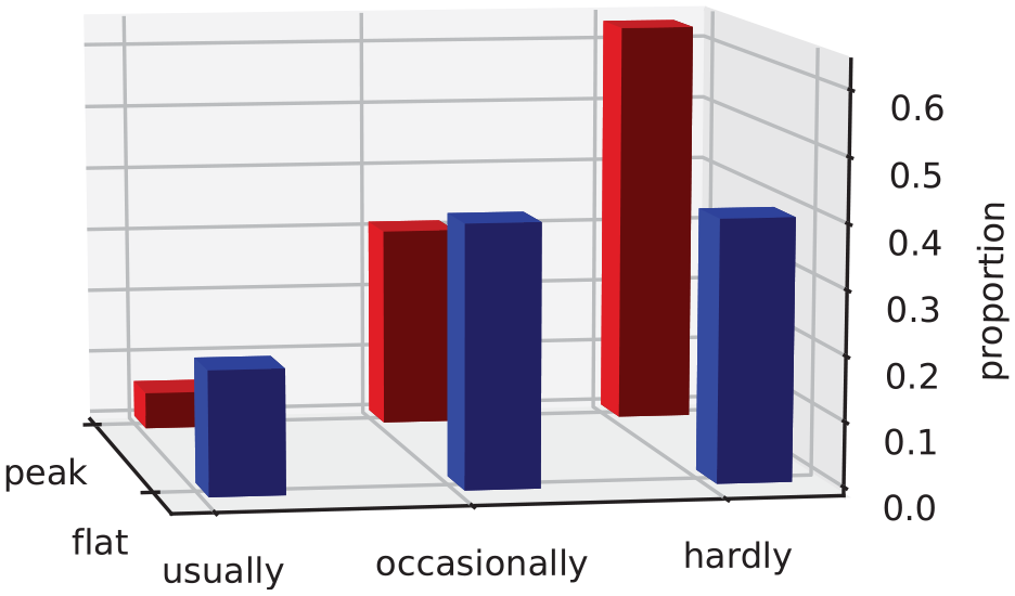
Questionnaire results.
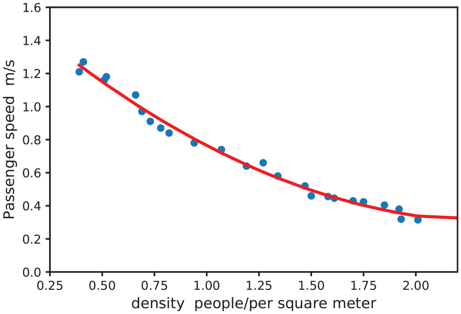
“Passenger-walking-speed” and “passenger-density” curve.
In this section, the train operation time is divided into peak and flat periods. In order to determine the period more scientifically and reasonably, the passenger flow intensities of stations are analyzed first. Figure 3 reflects the distribution of inbound passenger flow at different types of stations on weekdays. The types of station A, B, C, and D are respectively residence-and-work hybrid type, transportation hub type, residential type, and comprehensive commercial type.
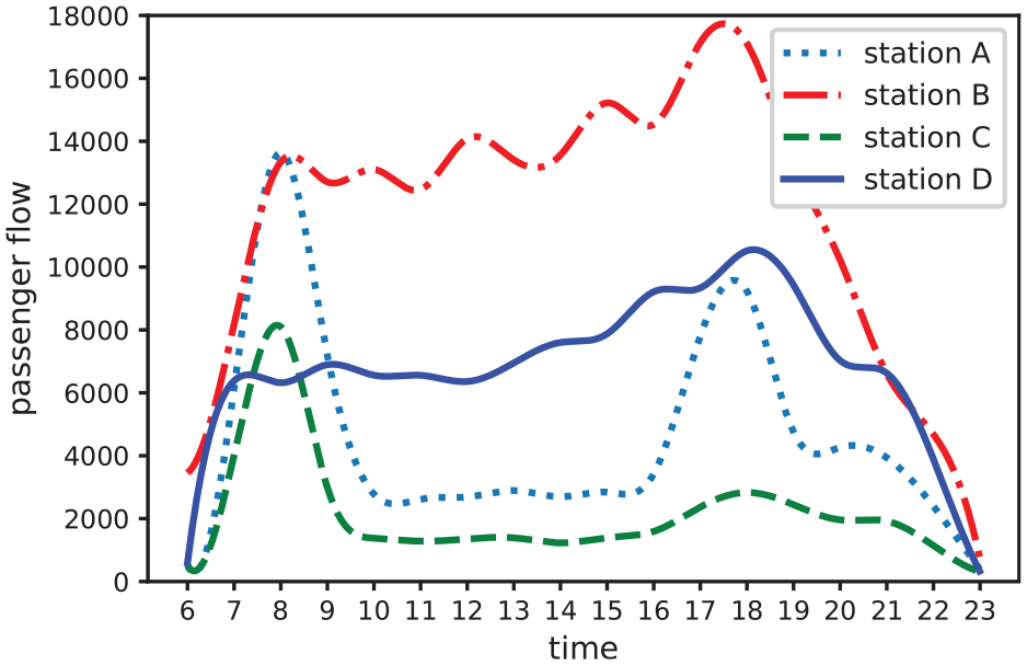
Distribution of inbound passenger flow at different stations on weekdays.
For station A, the inbound passenger flow curve shows a bimodal pattern, and the peak value at night is slightly lower than that in the morning. The passenger flow at other time is relatively flat. For transportation hub stations, there is no obvious peak in the curve, but the passenger flow intensity of the whole train operation time is at a high level. For residential stations, the inbound passenger flow curve presents a single-peak pattern. The peak is in the morning, and the intensity of passenger flow is relatively low and stable in other periods. For the comprehensive commercial station, the whole day passenger flow state is similar to the transportation hub type, but the passenger flow intensity is weaker than that of the latter.
The passenger flow on weekends demonstrates a significant difference from it on weekdays for the same station. Take station A for example, the passenger flow shows two obvious peaks on weekdays, which are distributed in the morning and evening. Whereas, the peak of the weekends passenger flow curve appears in the middle time of the whole day, and it is not obvious compared with other time. In addition, the overall passenger flow intensity on the weekends is significantly less compared with the weekdays, as can be observed in Figure 4.
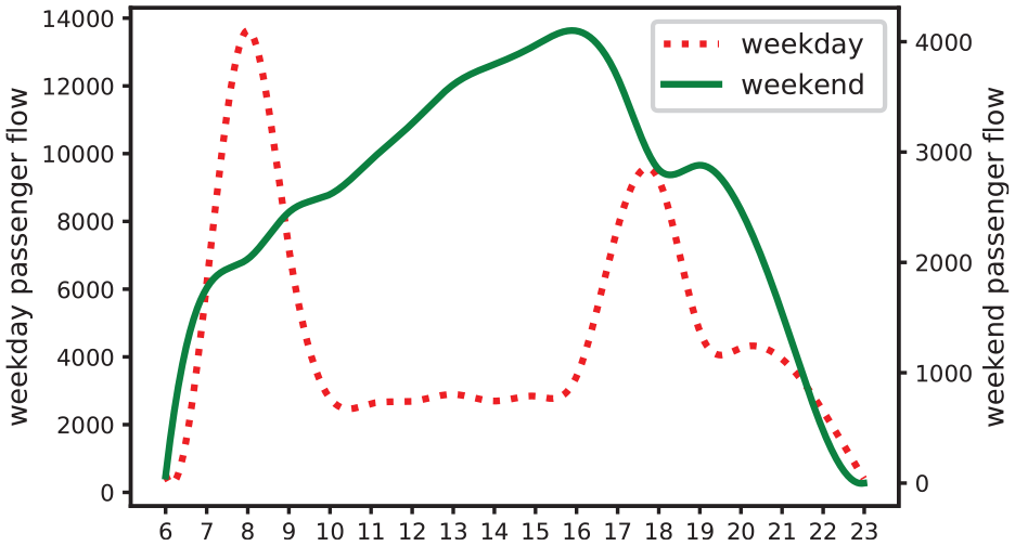
Distribution of inbound passenger flow in different days.
From above analysis, it can be seen that the peak period of passenger flow varies greatly among different types of stations on different types of days, which cannot be generalized. This paper identifies the peak and flat periods according to the following principles:
(1) The intensity of inbound passenger flow has a greater influence on the passengers’ arrival time and waiting time compared with outbound passenger flow. 18 Therefore, this paper identifies periods only based on the intensity of inbound passenger flow.
(2) Using τ as the time granularity, the train operation time is divided into several stages, denoted as
(3) Considering the situation that passengers enter stations during the peak or flat period and leave stations during another period. In order to simplify the analysis, passengers are classified according to their enter stations time in this paper.
Estimation of passenger route choice proportion in multi-period
Travel time parameters
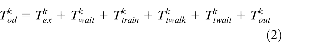
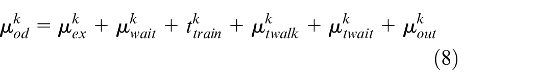
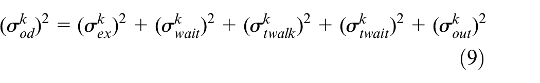
It is assumed that the travel time of passengers in urban rail transit consists of the following parts: entry and exit station walking time, waiting time at entry station, on-train time, transfer walking time and waiting time at a transfer station. It can be expressed as follows:
The researches7,9 show that passengers’ walking time
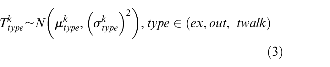
Assuming that the trains run according to the train schedule strictly, passengers’ on-train time can be obtained from the timetable, which is regarded as a constant in this paper and expressed as:

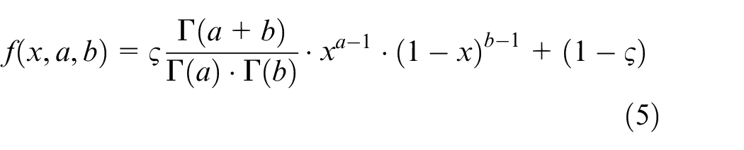
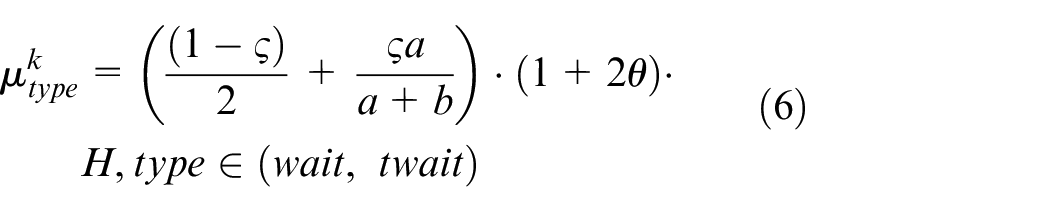
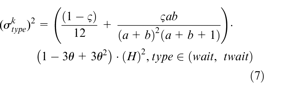
The waiting time on the platform is related to the train departure interval. Ingvardson et al. 19 proposes that there are two distinct passenger behavior types existing. One is that passengers arrive at the platform randomly and evenly, and the waiting time can be represented by the uniform distribution. The other is that passengers try to minimize their waiting time and will arrive when the train is about to leave, which can be represented by Beta distribution. The probability distribution of passengers’ waiting time can be expressed as follows:
Assuming that there is no overload delay phenomenon during the flat period and a part of passengers will wait for the second train during the peak period. Therefore, the expected value and variance of passengers’ waiting time can be expressed as:
Thus, the expected value and variance of passengers’ travel time can be expressed as:
Passenger travel time estimation
Due to the difference in stations’ layout and heterogeneity of passengers, the parameters such as entry walking time and transfer time are greatly different. Therefore, this paper adopts AFC data to infer passenger travel time. According to the number of feasible routes, the OD pairs can be classified as single-route ODs and multi-route ODs. Actually, feasible routes do not refer to all routes in the topological structure of two stations, but the routes that passengers may choose when traveling. If there is only one feasible route between an OD pair, it belongs to single-route ODs; otherwise, it belongs to multi-route ODs. As shown in Figure 5, although there are two routes from A to C in physical structure, passengers hardly choose route ④. So there is only one feasible route ① between AC and it belongs to single-route ODs. There are two feasible routes between AB (② and ③), so it belongs to the multi-route ODs.
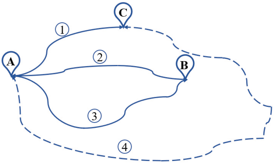
Single-route ODs and multi-route ODs.
By analyzing the probability distribution and parameters of single-route ODs’ travel time, the relevant rules of route travel time is obtained. Based on this, the travel time of each route between multi-route ODs can be estimated. The main steps are as follows:
Step 1: Search for the feasible routes between OD pairs.
Electronic map API is a free application program interface developed by map operators, which can quickly and accurately realize route searching, GPS positioning and other functions. This paper adopts the electronic map API to obtain the feasible routes between each OD pair, and adjusts the results with the consideration of the following rules: (1) Remove the travel routes which include other modes of transportation. (2) Since the results given by the map are based on the latest road network structure. If the road network now is different from the road network in the research period, we should adjust the results according to the historical information.
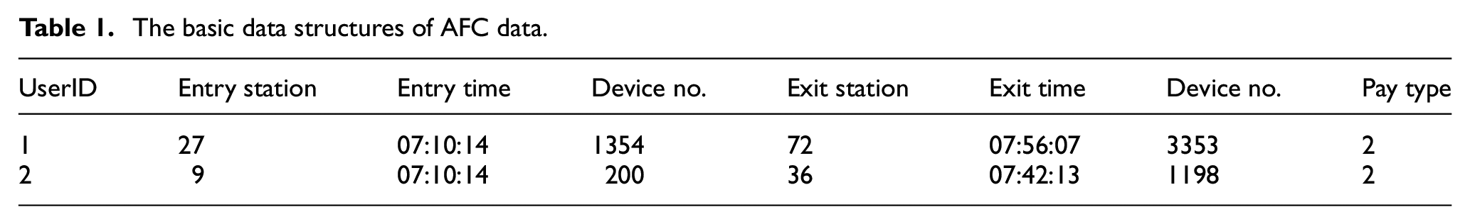
Step 2: Analyze the probability distribution and related parameters of single-route ODs’ travel time. The basic AFC data structure is shown in Table 1.
The basic data structures of AFC data.
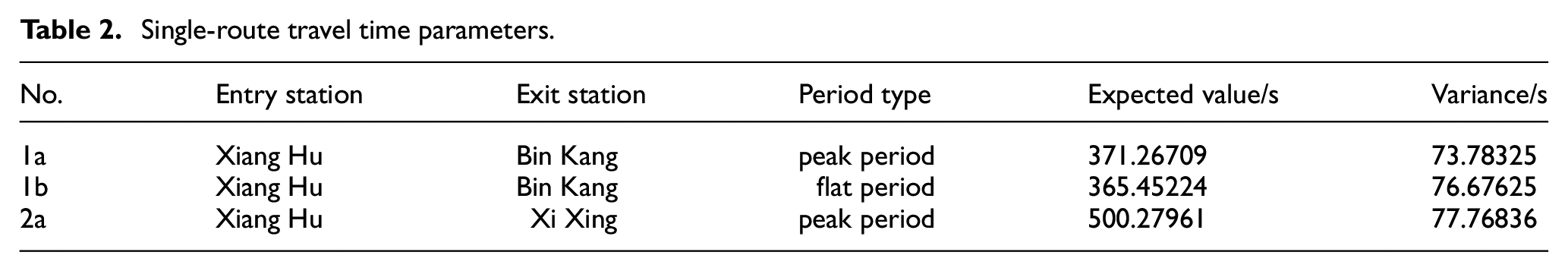
The total travel time of passengers for a certain OD pair can be obtained according to the arrival and departure swiping time. The AFC data of single-route OD can be fitted with normal distribution to gain the expected value and variance, as shown in Table 2.
Single-route travel time parameters.
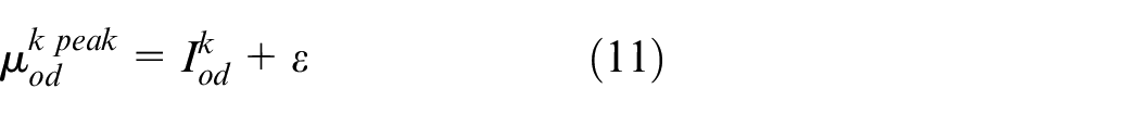
Step 3: Analyzing the expected value of travel time. When planning travel routes, the electronic map can not only give multiple feasible routes between OD pairs, but also estimate the travel time of each route. Comparing with the data in Table 2, we can find that the results of the electronic map are equal to the expected value in flat period approximately. Thus, we can consider:

The expected value in peak period is larger than the estimated time of electronic map. Through the correlation analysis, we can find the difference between them is related to the departure interval of trains at the entry station and follows the uniform distribution
Step 4: Travel time variance analysis. By analyzing the parameters of single-route ODs, it can be seen that the standard deviation of travel time is related to the departure interval of the entry train, the number of passenger transfers, the passenger density between OD pairs, the number of stations in the route. In this paper, random forest model was selected to fit the standard deviation of travel time and it can be expressed as follows:

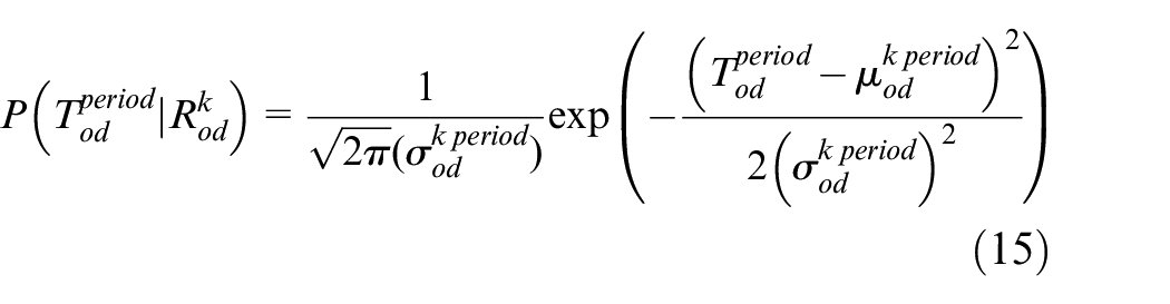
Step 5: According to formulas (10)–(12), the expected value and variance of travel time for each route between multi-route ODs can be estimated, and the probability distribution of travel time of all routes can be obtained.
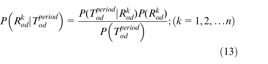
Estimation the proportion of passenger route choice
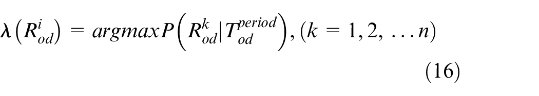
The Naïve Bayes algorithm is one of the most widely used classification algorithms. For the given training set, the joint probability distribution from input to output is trained based on the assumption of the independence between features. Then, based on the learned model, the output with the maximum posterior probability is calculated for an input. We propose an approach to estimate the proportion of route choice by introducing the Naïve Bayes algorithm. Taking the travel time as the attribute and the travel time of each passenger as the sample, we calculate the posterior probability of this sample belonging to each route and classify it into the route with the highest probability. The steps are described as follows:
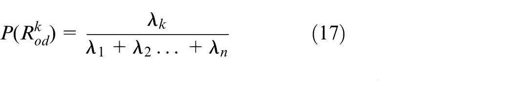
(1) Suppose the number of routes between an OD pair is n:
(a):

(b):
(2) Judge the classification of samples
(3) Label all samples and count the sample number on each route
(4) When the difference in the travel time of multiple routes is not significant, not all passengers will choose the route with the least travel time, but will choose a route according to their own preference. Therefore, when several posterior probabilities are approximately equal, only using the route corresponding to the maximum posterior probability as the passenger travel route will be quite different from the actual situation. Thus, after calculating the final posterior probability, this paper sorts it according to its value and confirms the passenger travel route in the following ways: If there are m feasible routes, which meet condition
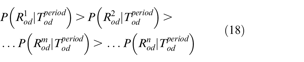
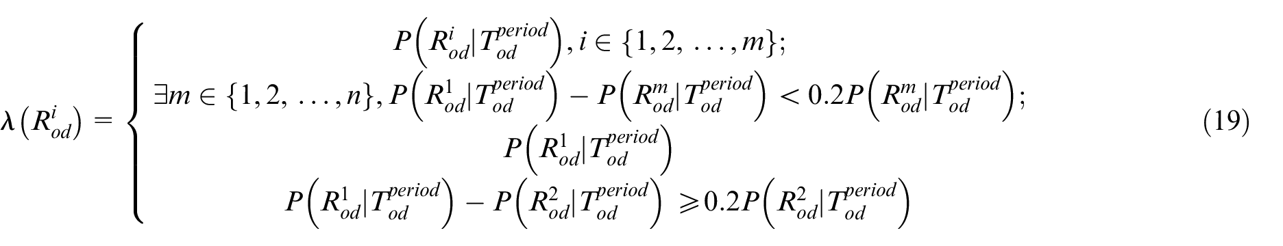
(5) Through the proposed method, we can get the corresponding routes of all samples and the number of samples on each route. Finally, we realize the estimation of the proportion of passenger route choice.
Case analysis
This paper takes Hangzhou Metro as an example to verify the proposed method empirically. Until January 2019, Hangzhou Metro had three lines, including Line 1, Line 2, and Line 4. It should be noted that line 1 contained two branch lines, which were the Xiashajiangbin branch line and the Linping branch line. The AFC card swiping data of passengers on 25 January 2019 is adopted for analysis. We choose a single-route OD pair (from Xianghu Station to Jinjiang Station) to show the route travel time distribution in multi-period. In order to analyze the travel time distribution of routes accurately, abnormal travel records are excluded in the study. Abnormal travel records indicate OD travel records whose travel time is longer than 95% of records or twice longer than the estimated time of the route returned by the electronic map API. Figure 6 shows that the probability density of passengers’ travel time has obvious normal distribution characteristics:
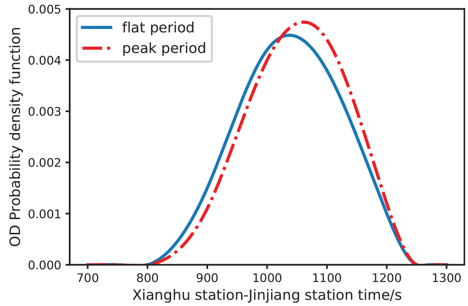
Probability distribution of passenger travel time from Xianghu station to Jinjiang Station.
Take the multi-route OD pair (from Jiangling Road to East Railway Station) as an example to estimate the proportion of passenger route choice. We use Amap API to acquire the routes between stations. Two feasible routes are obtained in this example, as shown in Figure 7. Route 2 transfers at the Jinjiang Station.
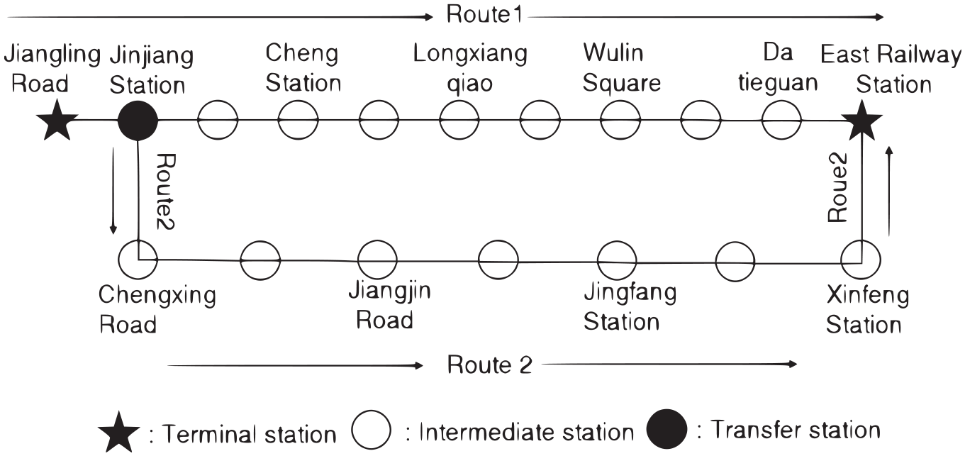
The routes from Jiangling Road to East Railway Station.
Jiangling Road inbound passenger flow is visualized in Figure 8. Two peaks in the passengers flow curve can be easily seen in the morning and evening. Thus, we can consider that Jiangling Road station is the residence-and-work hybrid type station, and most passengers are commuters in peak period.
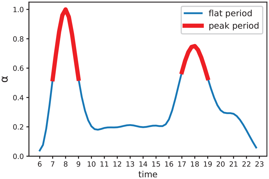
Peak and flat period identification result.
According to the passenger flow intensity of Jiangling road, the train operation time is divided into different stages with a granularity of 15 min and the normalized value of passenger flow
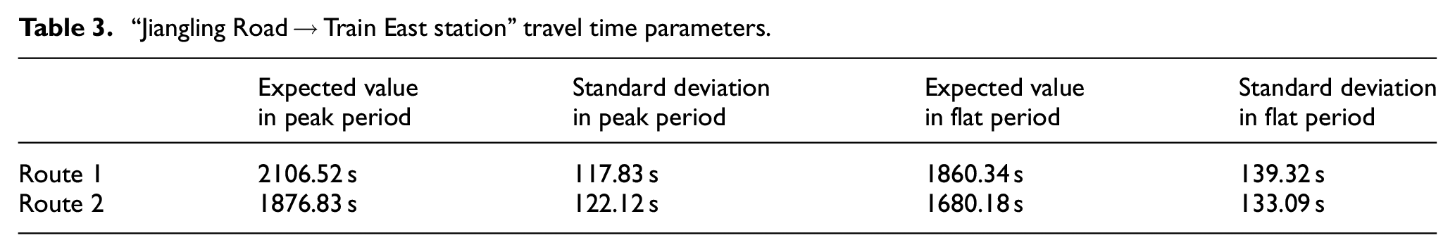
The parameters of the travel time are shown in Table 3. From Table 3, it can be seen that although passenger does not need to transfer by route 1, the expected value of it is larger than route 2 in both periods. In addition, the expected values of both routes are larger in peak period compared with the flat period.
“Jiangling Road → Train East station” travel time parameters.
A simulation experiment is designed to verify the proposed method. The simulation scenario is as follows: Randomly generate 1000 passengers, including 400 in peak period and 600 in flat period. The ratio of passengers choosing route 1 and 2 is
Jiangling Road to East Railway Station route choice result.
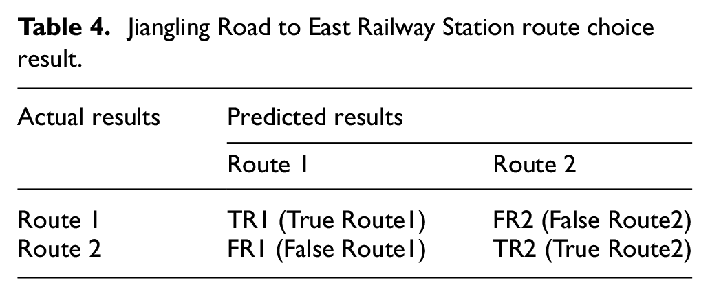
Jiangling Road to East Railway Station route choice results.
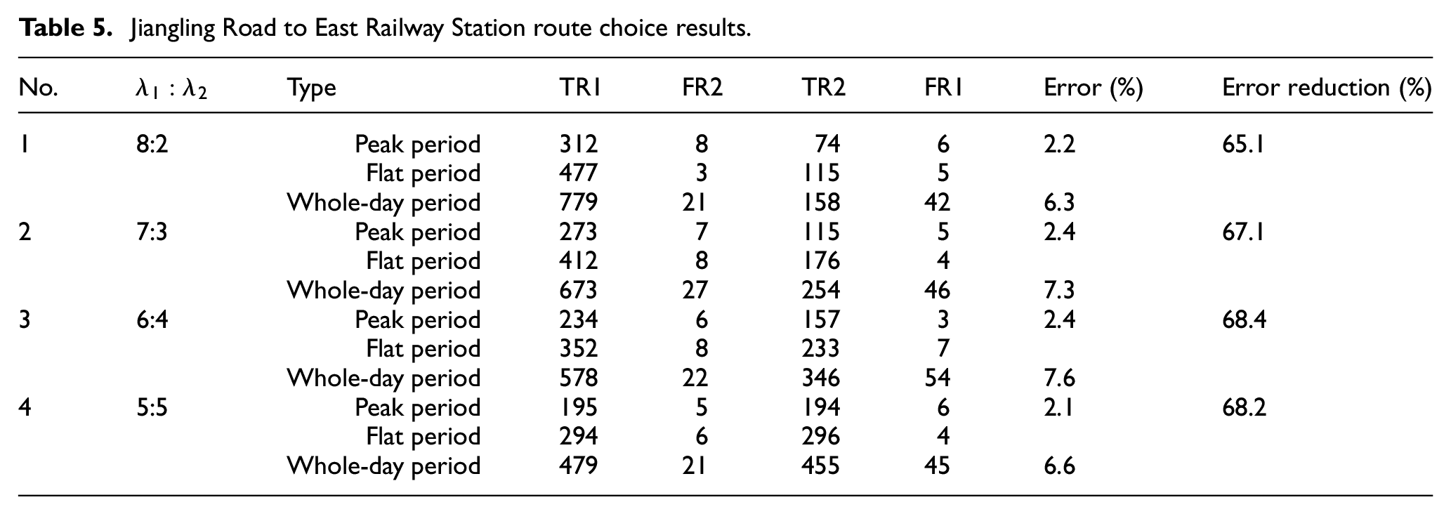
The “Whole-day period” refers to the contrast experiment of estimating passenger travel routes without dividing periods. The experiment
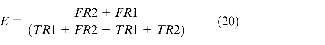
The denominator is the number of all samples and the numerator is the number of samples marked as false in the experiment. There are 24 samples misclassified in segment experiment and the number of all samples is 1000. By Formula (20), we can calculate that the error is 2.4%. Furthermore, we can acquire the error reduction with Formula (21).
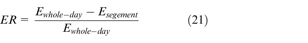
The result in Table 5 shows that the error of the segmented experiment is reduced by more than 60% compared with the whole-day experiment, which verifies the effectiveness of the method. Figure 9 shows the result of passenger travel route estimation.
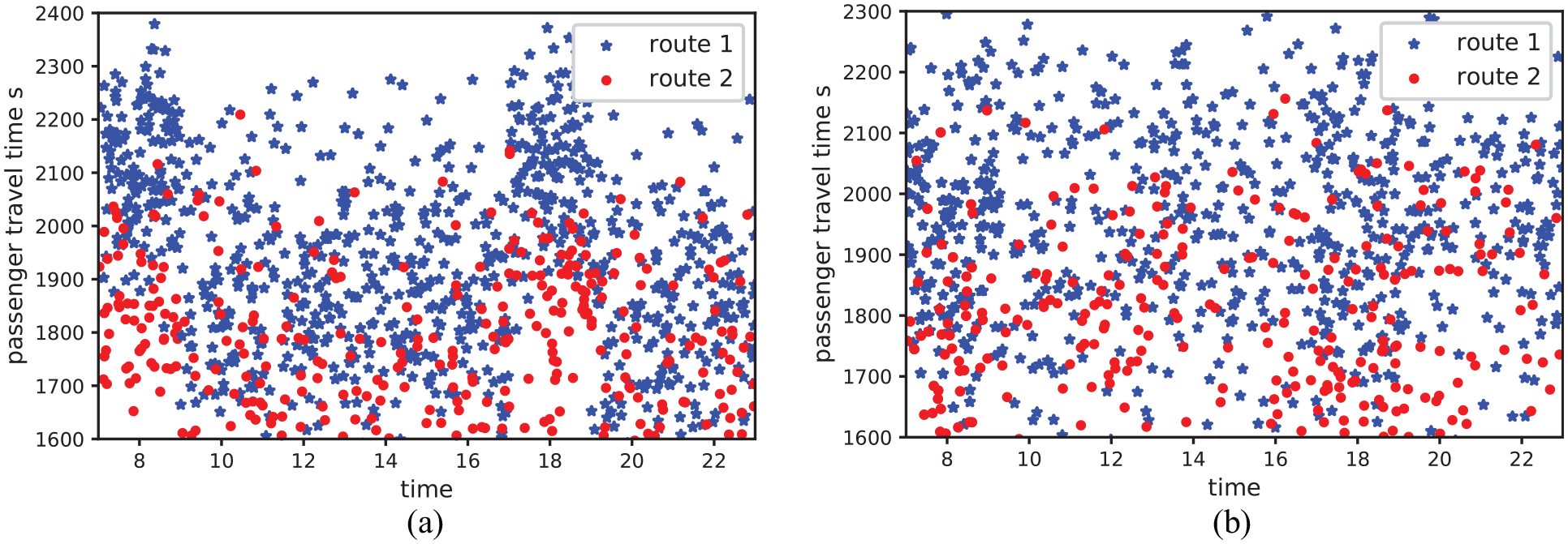
Passenger travel route identification result: (a) the segmented experiment and (b) the whole-day experiment.
Note that the bimodal distribution phenomenon can be clearly seen in Figure 9(a). In addition, some interesting findings are found in Figure 9(a). The travel time distribution of route 2 in peak period is similar to the distribution of route 1 in flat period, which are both concentrated between 1700 and 2000 s. However, there is no significant difference in travel time distribution between two periods in Figure 9(b).
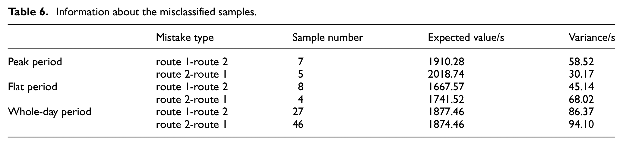
The relevant information and distribution characteristics of the misclassified samples can be observed in Table 6 and Figure 10.
Information about the misclassified samples.
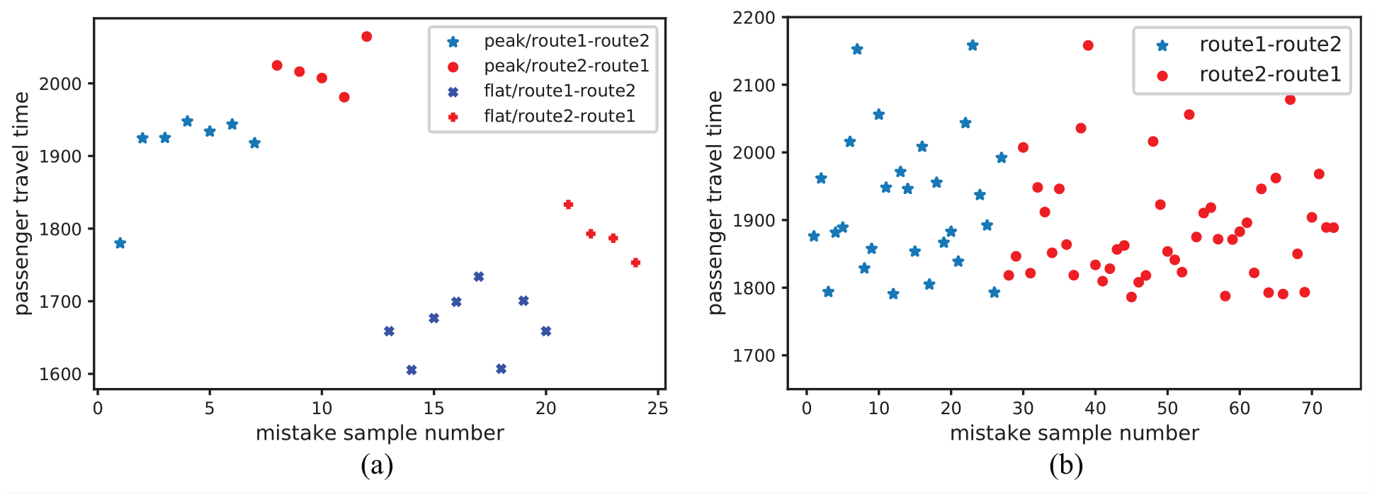
The misclassified samples distribution: (a) the segmented experiment and (b) the whole-day experiment.
From them, we can find these characteristics:
From Figure 10, we can clearly see that the number of misclassified samples in the segmented experiment is significantly less than that in the whole-day experiment. In the segmented experiment, the number of misclassified samples is 24, while in the whole-day experiment, the number is 73.
In the segmented experiment, the expected value of travel time for route 1 is larger than that for route 2 in both periods (as shown in Table 3). However, the travel time of the misclassified sample corresponding to route 1 is smaller than route 2, which is caused by the randomness of the experiment.
In the whole-day experiment, 27 samples are misclassified to route 2, and 46 samples are misclassified to route 1. The expected values are 1877.46 and 1874.46 s respectively, which are close to the expected value of travel time for route 1 in flat period and route 2 in peak period. Therefore, it can be considered that the above two types of samples are easy to be confused in classification.
Conclusion
In this paper, an estimation method for the proportion of route choice in multi-period urban rail transit control systems is proposed. In particular, in order to divide the train operation time into different periods, this paper formulate two indicators, which are the normalized value of passenger flow and the standard coefficient of peak passenger flow. This paper analyzes the probability distribution of travel times and obtains route choice through the Naïve Bayes algorithm. The simulation results show that the proposed method can effectively reduce the error rate caused by the similar travel time of different routes in different periods. However, when the travel times of several routes for a certain OD pair are almost equal, the accuracy of passenger travel route identification needs to be improved. In the future, we will consider combining passenger travel time with train schedules to optimize the approach.
Research Data
sj-docx-1-mac-10.1177_00202940221089501 – Supplemental material for Estimation and simulation for route choice proportion in multi-period urban rail transit control systems
Supplemental material, sj-docx-1-mac-10.1177_00202940221089501 for Estimation and simulation for route choice proportion in multi-period urban rail transit control systems by Yiyuan Yang, Ranran Sun, Peiyue Wang, Yang Yi and Guangyu Zhu in Measurement and Control
Footnotes
Declaration of conflicting interests
The author(s) declared no potential conflicts of interest with respect to the research, authorship, and/or publication of this article.
Funding
The author(s) disclosed receipt of the following financial support for the research, authorship, and/or publication of this article: This work was supported by the National Natural Science Foundation of China [No.61872037, No.61833002, No.62173167, No.62132003].
References
Supplementary Material
Please find the following supplemental material available below.
For Open Access articles published under a Creative Commons License, all supplemental material carries the same license as the article it is associated with.
For non-Open Access articles published, all supplemental material carries a non-exclusive license, and permission requests for re-use of supplemental material or any part of supplemental material shall be sent directly to the copyright owner as specified in the copyright notice associated with the article.