
Abstract
For wastewater treatment process (WWTP), mechanism model for activated sludge process (ASP) is unsuitable for estimating the effluent COD (Chemical Oxygen Demand) as the parameters of ASM (Activated Sludge Model) series models are varying with operating conditions. This paper presents an integrated model to predict the effluent COD. The model consists of two sub-models which are simplified mechanism model of ASP and RBFNN (RBF Neural Network) with variable structure (VSRBFNN). ASP model can express the dynamic biochemical reactions occurred in WWTP, and VSRBFNN is used to reduce the prediction error of the ASP model as an error compensation model. To reduce the complexity of the mechanism model of ASP, the parameters of mechanism model are fixed. The layout and the parameters of VSRBFNN can be adjusted according to the training data, and the stable learning algorithm can restrict the modeling error of VSRBFNN within a bounded domain. The output value of the integrated model is weighted sum of those of two sub-models, where the weights denote the contributions of the two “sub-models” to the prediction error of integrated model and are rectified according to the relative prediction error online. The structure of the integrated soft sensor is concise and real-time capability is improved. Simulations show that the presented soft sensor has satisfactory prediction accuracy under various operating characteristics.
Introduction
As a nonlinear process, WWTP operates under multiple operating conditions, and the reaction rates of microorganisms as well as the parameters fluctuate with different operating conditions. Some important water qualities of ASP cannot be measured by field instruments, which is unfit for the control of WWTPs. A soft sensor of effluent total phosphorus for monitoring was investigated based on partial least square and RBFNN. 1 A real-time monitoring system based on soft sensor model was presented in supervisory control and data acquisition system of WWTP. 2 The main characteristics of ASM models of WWTP are that the changing regularities and the interrelations of components are described by matrices. Switching functions are used in matrix reaction rates to reflect inhibiting effect caused by environmental changes, and avoid numerical instability in simulations when reaction expressions with on-and-off discontinuous features are used. 3 ASM series models show poor prediction accuracy when they are used to model the soft sensor of water qualities because ASM series models have complex structure and high dimensions, invariable parameter even when operating conditions fluctuates. Besides, the high-dimensionality of thorough phenomenological models needs a large computational cost. Meanwhile the interaction between dynamic variables of different time scales causes complex problems. 4 It is hard for ASM models to be identified in real-time, which is not beneficial for the practical application because of unknown parameters. 5 From the perspective of modeling, BSM1 (Benchmark Simulation Model No. 1) and its modified models are superior to previous ones. But the parameters of ASM series models and BSMs model are varying with influent water qualities and operating variables. At the same time, the external disturbances of WWTP, strong nonlinearity and time delay are not considered. 6 Above mechanism models show poor prediction performance when applied to the modeling of WWTP directly. Meanwhile, the large computation cost of multi-dimension differential equations deteriorates the real-time capability of mechanism models of the activated sludge process, specially under various operating conditions.
Soft sensors based on data-driven methods gain great attentions. A predictive models for wastewater flow forecasting based on time series analysis (autoregressive integrated moving average) and artificial neural network was presented, while for the ARIMA model, the time series must be stationary. If the data is still not stationary after certain transformations, ARIMA cannot be used. 7 A price prediction model of crude oil based on support vector regression (SVR) with a wrapper-based feature selection approach using multi-objective particle swarm optimization (PSO) technique was developed, but the theoretical proof of PSO is difficult to achieve. 8 For the modeling of WWTP, RBFNN based on adaptive computation algorithm was used in online monitoring of effluent total phosphorus. 1 Fuzzy neural network with adaptive learning rate used in online fault detection of WWTP. 9 Neural network, 10 hybrid genetic algorithm, 11 SVM, ANFIS, 12 adaptive PLS, and PCR are applied to predict effluent COD of WWTP. A modeling method including partial least squares, support vector regression, and artificial neural networks with a meta-learning algorithm was used to predict the effluent indices in papermaking wastewater treatment processes, yet the execution efficiency of real-time monitoring and the expansion of sample size should be considered further. 13 The neighborhood component analysis was used to model papermaking wastewater treatment processes, whose modeling accuracy precedes over PLS and neural network, yet the online parameters adjustment are not included. 14 Bates and Granger presented the multi-models method by integrating several models, so as to the prediction accuracy and robustness can be improved. 15 Soft sensors of water qualities using multi-models are investigated widely under multiple operating conditions of WWTP.16,17 The performances of soft sensors based on data-driven methods are influenced by the quantity and quality of training data.
Recently hybrid integrated models are researched widely which the mechanism model and intelligent models are used as sub-models. A hybrid deep learning model based on sequential fusion convolutional neural network, long short term memory and attention mechanism was proposed to monitor the water quality of paper industrial wastewater treatment system, but the online prediction algorithms based on deep learning algorithm is not researched. 18 A hybrid model for wind speed forecasting was investigated to improve the forecasting performance of wind power, where long short-term memory (LSTM) neural network and decomposition methods are integrated with gray wolf optimizer optimizing the intrinsic mode function (IMF) estimated outputs. Theoretical proof should be considered further. 19 An integrated soft sensor of COD, MLSS, and cyanide concentration was introduced that ASM1 and data-driven model are arranged in parallel. 20 Error compensation model built by FFNN, RBFNN, PLS, and NNPLS respectively is adopted to compensate the deviation between the effluent water qualities computed by ASM1 and real data, which the prediction accuracy is enhanced greatly. However, ASM1 model is very complex with high order and more computation time is needed. An integrated model of water quality was presented whose error is compensated by RBF neural network, while the structure of RBFNN is determined by experience. 21 A hybrid soft sensor for COD is presented in literature, 22 in where mechanism model and linear polynomial models are integrated. Linear models are used to compensate the modeling error of mechanism model and the number of linear models can be adjusted by synchronous clustering algorithm that the time interval between input and output data and the relevance of adjacent data is considered. But the set of linear models shows weak ability of nonlinear description.
In order to model the online soft sensor of water qualities under varying with operating conditions and improve the real-time capability, an integrated model of COD is proposed in this paper, where SASM1 (Simplified ASM1) and VSRBFNN are taken as two sub-models. The weighted sum of the outputs of sub-models is used as the output of hybrid model, and the weights of each sub-model are modified according to the relative prediction error. SASM1 expresses the biochemical reactions of ASP, and VSRBFNN is used as error compensation model of SASM1. The structure of the integrated soft sensor is concise compared with the model of ASP based on ASM1, meanwhile the stable learning algorithm can restrict the modeling error of VSRBFNN within a bounded scope, so real-time capability is improved. Simulations show that the integrated soft sensor has satisfactory prediction ability under various operating characteristics.
The layout of this paper is designed as: section 2 describes the technological flow of A/O (anoxic/aerobic) process; section 3 presents the modeling strategy of the integrated soft sensor; section 4 describes the simulations; and section 5 summarizes the conclusions.
Descriptions of A/O process
Process description
The flow chart of the A/O process is as shown in Figure 1.
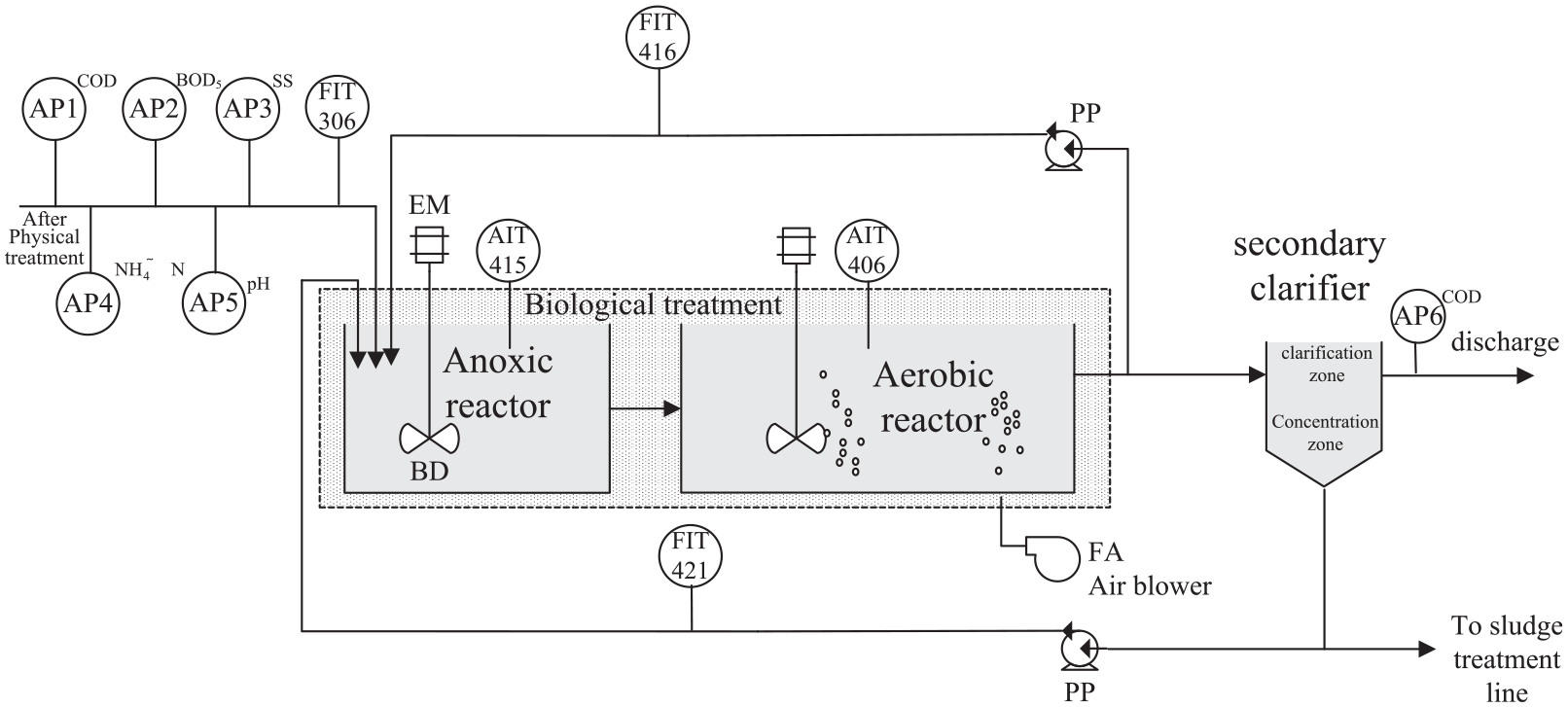
The flow chart of the A/O process.
In A/O process, the wastewater after primary treatment enters into anoxic reactor, is mixed with activated sludge from secondary clarifier and the internal reflux from the aerobic reactor, which provides sufficient carbonaceous organic material for denitrification in anoxic reactor. Meanwhile, anoxic and aerobic reactors possess enough microorganisms and anoxic reactor receives nitrate generated by nitration reaction in aerobic reactor.
In anoxic reactor, denitrification reaction occurs and most nitrogen pollutant and a portion of carbon pollutant are removed. The wastewater in anoxic reactor flows into aerobic reactor. Nitration and carbon degradation reactions take place in aerobic reactor and most carbon pollutant is degraded. Air blowers are used to regulate DO (Dissolved Oxygen) in aerobic reactor. Portion of wastewater from aerobic reactor is recycled back to anoxic reactor to participate in denitrification, the remaining wastewater enters into secondary clarifier and is settled by gravity.
Input-output relationship of COD soft sensor
In order to predict COD, the input-output relationship of soft sensor should be decided in advance.
The subsidiary variables of COD soft sensor can be selected as DO of aerobic tank, influent flow rate Qin, influent SS, COD, NH+4-N, etc.
21
The relationship among subsidiary variables and effluent COD

Here, f(•) is dynamic nonlinear function. 14
The modeling strategy of integrated soft sensor
The modeling strategy of soft sensor in this paper is shown in Figure 2.
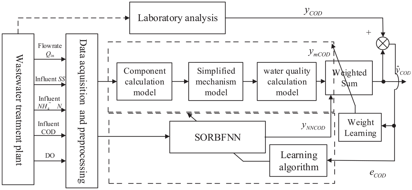
The modeling strategy of integrated soft sensor.
The raw data from WWTP after preprocessing can be used for modeling. ASP model and VSRBFNN are taken as the sub-models, and the output of the integrated model is the weighted sum of those of sub-models. The weights are trained with modeling error. VSRBFNN is used to reduce the error of the mechanistic model, whose structure and parameters are adjusted by the modeling data.
Here,


Here, a1 and a2 are the weights of mechanism model and VSRBFNN,
Mechanistic model of ASP process
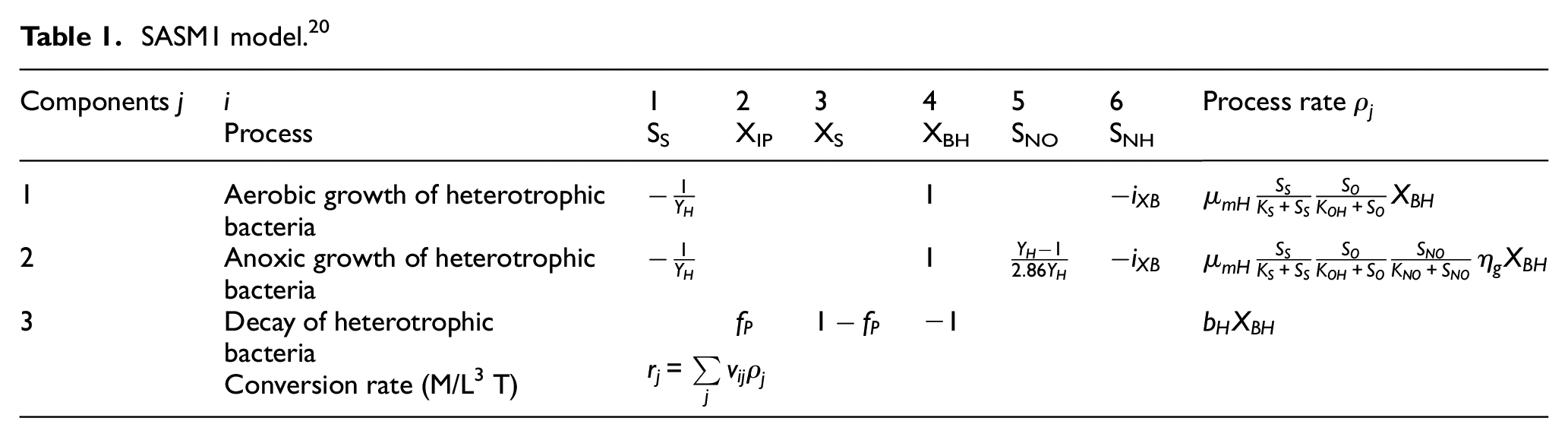
Although ASM1 models show poor prediction accuracy when used to model the soft sensor of water qualities, the model of ASP based on ASM1 can express the basic dynamics trend of activated sludge process. A simplified ASM1 (SASM1) is built,22,23 shown in Table 1. The mechanism model of ASP process is built based on SASM1 whose parameters are set to the values of ASM1 at the temperature of 20°C. 23
SASM1 model. 20
VSRBFNN
VSRBFNN is used as error compensation model to decrease the modeling error of the ASP model.
RBF neural network
As a feedforward neural network, RBFNN can approximate any nonlinear function. RBFNN precedes other feedforward neural networks on the uniform approximation capability of nonlinear continuous function, 24 and radial basis function is usually used as activation function of hidden layer. RBFNN has the characteristics of fast convergence, high approximation accuracy and simple network structure. RBFNN is widely used as the soft sensor of key parameters in industrial processes. 25 It has been proved that RBFNN with stable learning algorithm can guarantee the stability of the modeling error when unmodeled dynamics and uncertain disturbances exist. 26 So RBFNN can be used as error compensation model in integrated soft sensor because of the unknown fluctuation characteristics of real WWTP.
The performance of RBFNN is decided by parameter optimization algorithm and the structure size. In RBF neural identification and modeling, one of the other important issues is the effect of network structure on computational loading and generalization.
The following single-output discrete nonlinear system is considered:
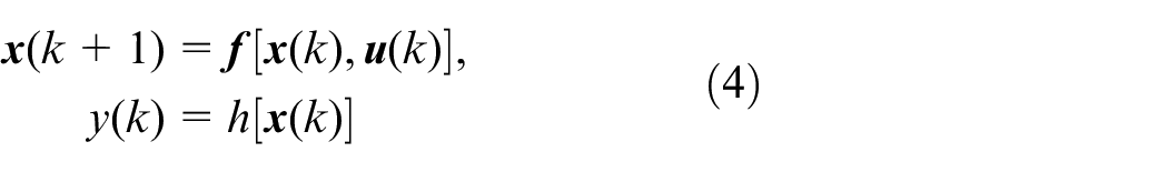
Here,
Single-output RBFNN described by (5) is used to identify the nonlinear system (4),

Here,
Here,
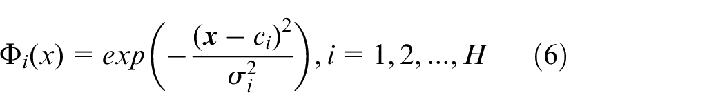
Activation function of hidden nodes are the radial basis function, which determines the mapping relationship between input variables and hidden space. Hidden layer and output layer shows linear relationship, and the output of RBFNN is the weighted sum of outputs of hidden nodes.
The adjustable weights can be solved by linear equation set or learned by recursive least squares method if the number of hidden nodes, the center and width of radial basis function are known, which can speed up learning and avoid falling into local minimum. In order to enhance the adaptivity and approximation accuracy of RBFNN, the node number of hidden layer, the center and width of radial basis function should be updated during the learning process. Among, the nodes number in hidden layer is fixed or adjusted dynamically during learning.
Structure design of VSBRFNN
The training samples of VSRBFNN are N input/output data pair (x,y), x is the input vector with n dimension, y the desired output with m dimension, j the nodes number of hidden layer. At the beginning of the training stage, the hidden layer has no nodes. When the first data sample comes into RBFNN, the input vector is taken as the center vector of the first hidden node and the output vector as the connection weights of hidden nodes and output node. At k time instant, it supposes there are j nodes of hidden layer in RBFNN. When the kth data sample comes into RBFNN, the kth input vector is compared with the center vectors of the existing j hidden nodes by similarities. The similarity is expressed as:
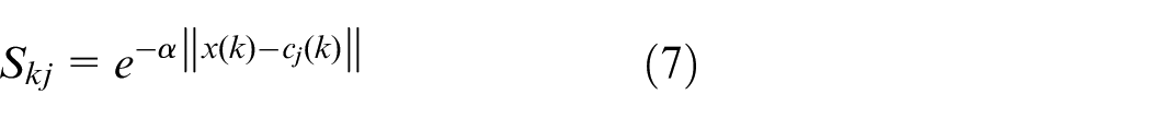
Here,
The range of Skj is (0,1], Skj is the bigger, the distance between x(k) and cj(k) is the closer and the degree that x(k) activates the jth node is the deeper. Here the maximum of the similarity is

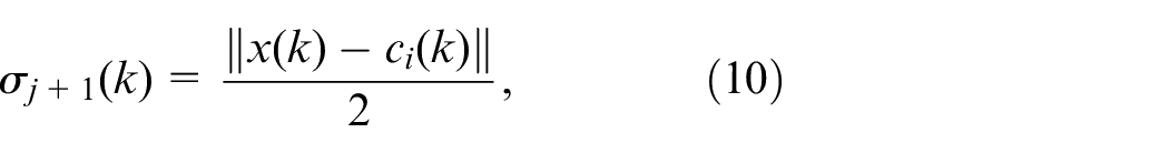

Here ci(k) is the center of the node closest to the new sample x(k).
If

Here,
The design procedure of VSRBFNN is:
① Initial moment, the nodes number of hidden layer in RBFNN
② When the first data sample comes into RBFNN, the nodes number of hidden layer is increased by 1. the input vector is used as the center vector of the first hidden node, meanwhile the output as the connection weights between hidden layer and output layer;
③ When the kth data sample comes into RBFNN, the similarity between the kth input vector and current all hidden nodes as well as the hidden node with the biggest similarity
④ If
⑤ If
The above design procedure seeks a concise structure for RBFNN and the initial parameters can speed up the learning of RBFNN.
Parameter learning algorithm of VSRBFNN
The structure of VSRBFNN is designed in previous section and the parameters are learned by stable learning algorithm. The index is defined as:
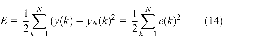
Here,

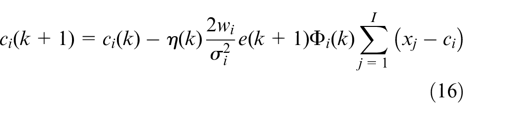
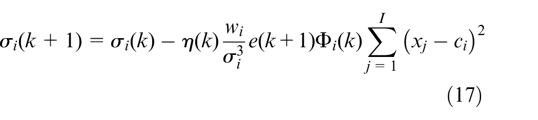
Here,


Above learning algorithm can restrict the modeling error e(k+1) of VSRBFNN within a bounded domain.
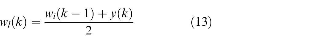
Online adjustment method of integrated weights
In (2), the integrated weights of ASP model and VSRBFNN satisfies
① The prediction relative error of ith sub-model at time k is calculated by:
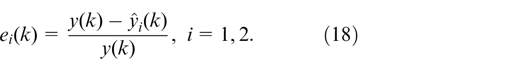
If,
② The ratio of prediction relative error of ith sub-model at time k is calculated by:
③ The entropy of prediction relative error of ith sub-model at time k is calculated by:
④ The weight ai(k) of ith sub-model at time k is calculated by:
Here, r denotes the number of sub-models, r = 2.
After adjusting the integrated weights, the output of the integrated model is calculated by (3).
Simulations
The data set from south wastewater treatment plant of Shenyang are used to verify the integrated modeling method. 150 input/output data pairs are taken as training dataset and 100 data pairs are used in online soft sensing of effluent COD.
The parameters of ASP model are: μmH = 6, bH = 0.6, KS = 20, KOH = 0.2, KNO = 0.5, YH = 0.67, fP = 0.08, iXB = 0.086.
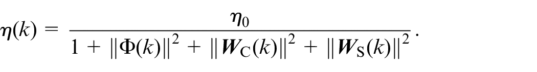
The threshold value of the similarity SV = 0.65, learning rate η0 = 0.9, the initial weights of sub-models are equal a1(0) = a2(0) = 0.5.
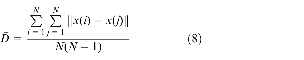
Influent COD, Influent SS, ammonia nitrogen NH+4-N, flowrate Qin, DO in aerobic tank are used as the inputs of integrated model. The influent water qualities show large fluctuations. The range of influent NH+4-N is 14.8–54.7 mg/L, and that of flowrate Qin is 606–3637 m3/h. The training data of NH+4-N and Qin are shown as Figure 3. Component calculation model can convert five variables into the components in SASM1. The inputs of VSRBFNN are above five variables. That is, the initial structure of VSRBFNN is 5-0-1. Then, the structure and the parameters of VSRBFNN are determined according to the methods presented in section III. The integrated weights of mechanism model and VSRBFNN can be learned by the procedures presented in section III.
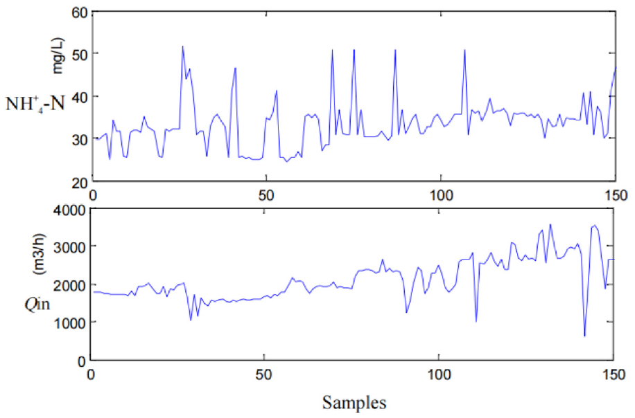
The training data of NH+4-N and Qin.
The number of hidden nodes in VSRBFNN at the training stage is shown in Figure 4 where the number of the hidden nodes is fixed at 7 from the 86th data sample. It indicates seven hidden nodes of VSRBFNN can describe the most operating characteristics of concerned WWTP. Compared with RBF neural network whose structure is fixed and determined according to experience, the complexity of VSRBFNN with varying structure is reduced to some extent. So the real-time capability of VSRBFNN is improved.
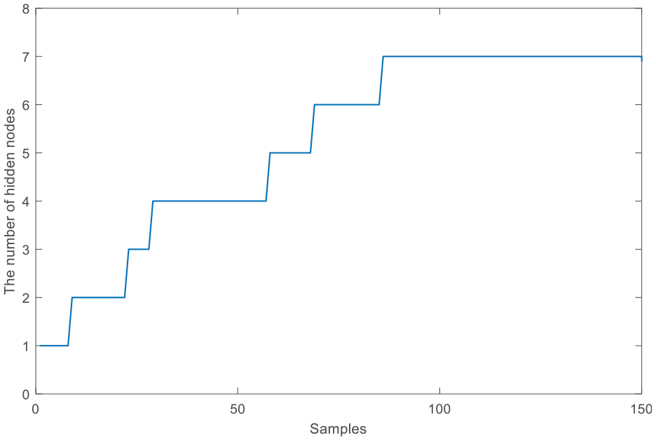
The hidden nodes number in VSRBFNN.
The training error of integrated model is shown in Figure 5. The span of the training error is about (0.5 13.2).
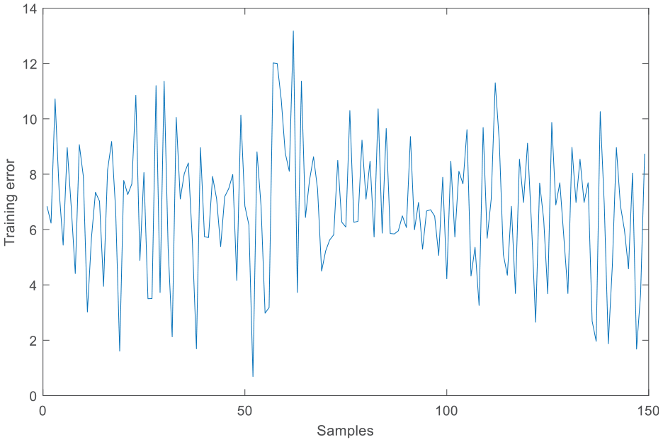
The training error of integrated model.
The comparison of soft sensing result and real effluent COD is shown in Figure 6. The soft sensing value of integrated model can track the real effluent COD well under the varying operating conditions, which indicates the integrated model has satisfactory prediction accuracy.
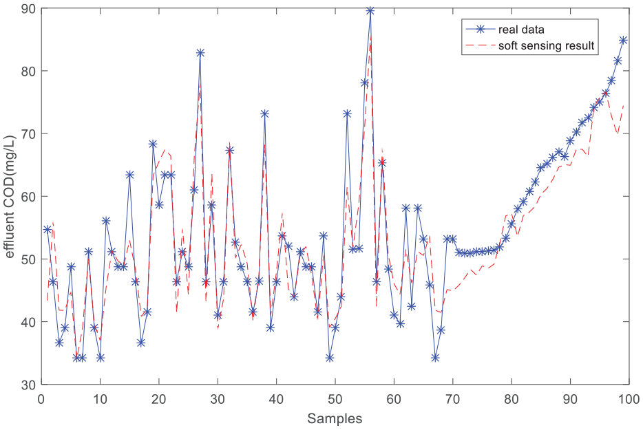
The comparison of soft sensing result and real effluent COD.
The weights of two sub-models in integrated model are shown in Figure 7. The initial weights both are 0.5, and are rectified according to the prediction errors of corresponding sub-models. The sum of the weights stays at 1. Each weight fluctuates along with the prediction error of sub-model, which indicates the reliability of each sub-model is decided by corresponding prediction errors. The prediction relative error of the sub-model is the larger, the corresponding weight is smaller, which indicates the effect of the sub-model on the output of the integrated model are the smaller. And vice versa.
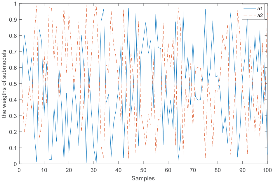
The weights of the sub-models in integrated model.
The stable learning rate η(k) of VSRBFNN is shown in Figure 8. The learning rate is not fixed and varying with modeling error of VSRBFNN. η(k) is larger than the learning rate of common BP algorithm. If the learning rate of common BP is bigger than 0.2, the corrected value is too big and causes vibration and divergence. The stable learning rate changes between 0.07 and 0.4 and can realize one-step optimization without divergence. The modeling error can be restricted within a bounded scope.
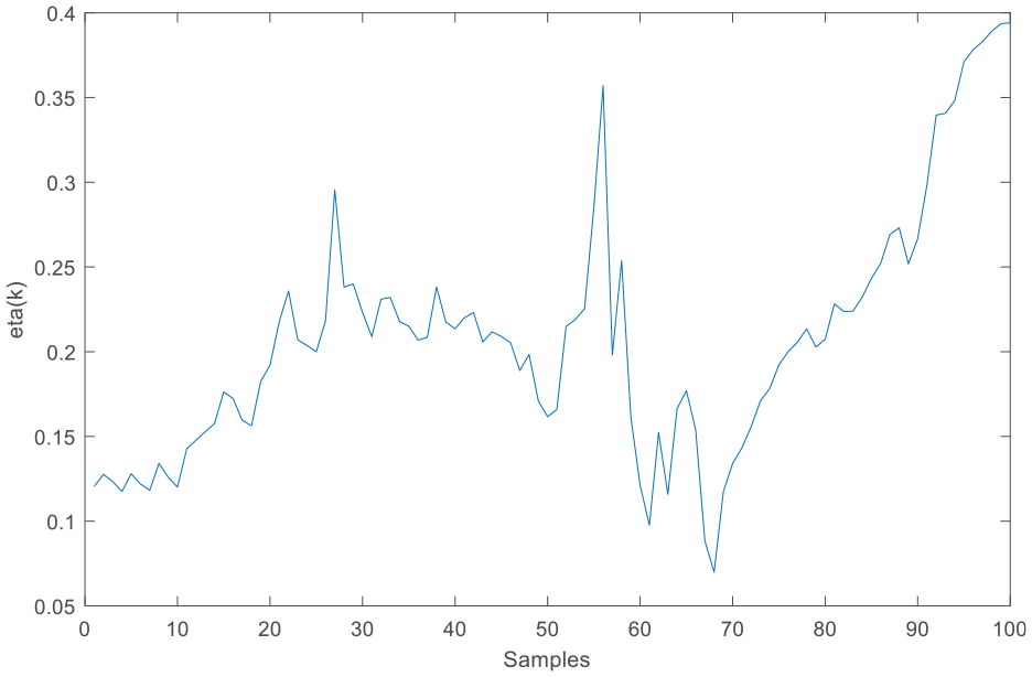
The stable learning rate of VSRBFNN.
Discussions
The comparisons of training and testing RMSE using different methods are listed in Table 2.
The precision comparisons.
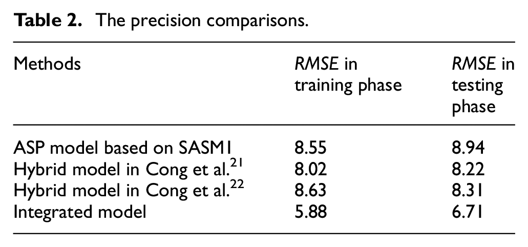
There is no obvious difference between training and testing RMSE of ASP model based on SASM1 because the parameters of SASM1 are fixed. In Cong et al. 22 the modeling error of ASP model is compensated by linear models, so the prediction accuracy is improved to some extent.
Hybrid soft sensor of water quality integrates mechanism model and VSRBFNN shows satisfactory predictive ability under varying influent conditions, which precedes above mentioned methods. The reasons are that VSRBFNN is adopted as error compensation model to express the nonlinear characteristics of WWTP precisely and stable learning algorithm guarantees the modeling error of VSRBFNN within a bounded scope. Compared to Cong et al.21,22 the testing RMSE is lowered by 22.5% and 23.8%, respectively. Meanwhile, the online adjustment method of integrated weights carries out according to the entropy of prediction relative error instead of error back propagation algorithm, which overcomes the shortcomings of the error back propagation.
Conclusions
Integrated soft sensor of COD was presented in this paper. From the simulations, the conclusions can be obtained and shown as follows: (1) As an error compensation model, VSRBFNN is taken as a sub-model in integrated model because mechanism model has complex calculation and low accuracy. (2) The structure and parameters of VSRBFNN are learned online according to the real data. (3) When more operating information are included in training data, the nodes number of hidden layer of VSRBFNN will be large. So the method of removing the redundant hidden nodes should be considered further.
Footnotes
Declaration of conflicting interests
The author(s) declared no potential conflicts of interest with respect to the research, authorship, and/or publication of this article.
Funding
The author(s) disclosed receipt of the following financial support for the research, authorship, and/or publication of this article: Project (61803191) supported by the National Natural Science Foundation of China; Project (2019-KF-03-05) supported by Natural Science Fund Project of Liaoning Province.