
Abstract
The purpose of this research is to develop a high-efficiency, low-cost, and easy-to-use tracking system for vehicles, and it is expected that the system can be extended to areas such as service robots, autonomous driving, and manufacturing. In this paper, we introduced an object detection algorithm based on convolutional neural networks to realize face recognition, which has better efficiency and robustness than traditional machine learning methods. With the concept of edge computing, we deployed the model on the local embedded system to improve the information transmission and security issues of cloud computing. In order to realize the tracking system, this paper builds a mecanum-wheel vehicle with omnidirectional mobility, and proposes a parallel-cascade PID controller architecture based on the mecanum-wheel vehicle. The fixed distance linear tracking control can be realized through the dual-loop feedback control of distance and yaw angle; moreover, the vehicle slipping which is caused by difference rotation speed can be improved. Finally, through algorithm optimization, controller parameter adjustment, and system integration, an omnidirectional mobile vehicle with recognition and tracking functions is realized. The experiment results indicate that the system is stable and robust during actual operation.
Keywords
Introduction
In recent years, the development of deep learning technology has made the field of service robots and self-driving cars more diversified and popular. The recognizing and tracking of dynamic objects are important for robots and vehicles. With these technologies, we can perform some complex tasks such as home care, 1 rescue, 2 transport, 3 bio-miedical, 4 and information,5,6 etc. Moreover, we can reduce the use of specialized sensors with the aid of images, and even let the machine autonomous. 7
In the early face recognition stage, it is often necessary to perform face detection before face recognition. Most of the face detection algorithms are used with manual Haar-like features 8 or HOG (Histogram of Oriented Gradient) 9 to perform features extraction, and then trained the classifier such as Adaboost (Adaptive Boosting) 10 or SVM (Support Vector Machine) 11 to realize face detection. After obtaining the face area, the image needs to be pre-processed, such as cropping, face alignment, noise removing etc., and finally face recognition is realized through matching similarity such as PCA (Principal Component Analysis) 12 or LBPH (Local Binary Patterns Histograms). 13 Although these traditional machine learning methods have good performance, the steps are complicated and the anti-interference ability of external factors is poor, so that they are not suitable for dynamic detection. Compared with traditional machine learning methods, the object detection methods based on deep learning are simple and perform better.
The requirements of certain applications and advances in technology have led to the development of object detection algorithms that are widely used in computer vision tasks such as face detection, face recognition, autonomous driving, and image labeling. Object detection is usually performed using a two-stage detector or one-stage detector. In two-stage detection, a model first proposes candidate object bounding boxes through a region proposal network and extracts features through region of interest pooling to classification and bounding-box regression tasks; an example of a model that employs two-stage detection is Faster R-CNN.14,15 In one-stage detection, a model proposes predicted boxes from input images directly without the region proposal step; examples of models that employ one-stage detection include SSD 16 and YOLO. 17 Two-stage detectors have high localization and classification accuracy but low inference speed, whereas one-stage detectors have high inference speed but a lower accuracy than two-stage detectors.
In order to achieve real-time detection performance on embedded systems with limited computing power, this paper uses one stage detector YOLOv3 18 algorithm to achieve face recognition, and some experimental optimizations are made for the YOLOv3 algorithm depend on the task, as shown in Table 1. Therefore, these optimizations eventually increase mAP by 8.5% on the custom data set. In addition, we deploy the trained model on the embedded systems and use deep learning accelerator to increase the operation speed by five times.
Performance comparison of improvement.
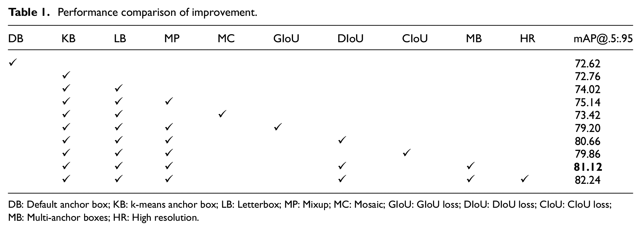
DB: Default anchor box; KB: k-means anchor box; LB: Letterbox; MP: Mixup; MC: Mosaic; GIoU: GIoU loss; DIoU: DIoU loss; CIoU: CIoU loss; MB: Multi-anchor boxes; HR: High resolution.
In this paper, we build a mecanum wheel vehicle with omnidirectional mobility and proposes a parallel-cascade PID architecture as the control system of the vehicle to achieve tracking function. The difference from the general PID architecture, the parallel-cascade PID architecture is allowed to input multiple control signals and has multi-loop, these characteristics make the system more effective in reducing the effects of disturbances and more stable; however, it is not easy to adjust parameters due to cascade architecture. The most important thing for a good tracking system is the immediacy and stability of operation. Therefore, the following experiments will focus on how to improve the accuracy of the model and good controller design and parameter adjustment.
Methodology
YOLOv3
YOLOv3 was proposed by Redmon et al. 19 . YOLOv3 has a fully convolutional network architecture, Darknet-53, inspired by ResNet. Using residual skip connections, we can solve the vanishing gradient problem and increase the depth of the network. For object detection, YOLOv3 uses a multiscale prediction method similar to that of a feature pyramid network (FPN), 20 as shown in Figure 1. Shallower feature maps have higher resolution, which is conducive to localization; however, deeper feature maps have richer semantic information, which is conducive to classification. Therefore, an FPN combines these advantages and detects objects on three different scales, thereby mitigating the issues that make it difficult to detect small objects.
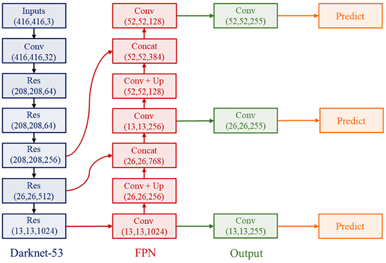
YOLOv3 network structure.
To allow a network to learn easily and achieve high detection accuracy, YOLOv3 inherits the YOLO9000 21 method of determining the anchor box and uses k-means clustering on the training set to automatically obtain good priors. The author selected nine clusters and evenly assigned these clusters to three scales for prediction using the YOLOv3 algorithm. The loss function of YOLOv3 consists of coordinate loss, confidence loss, and classification loss.
Coordinate loss is defined as follows:
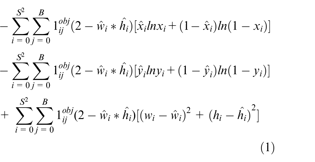
where,
Confidence loss is defined as follows:
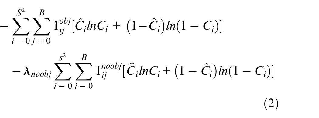
where
Classification loss is defined as follows:
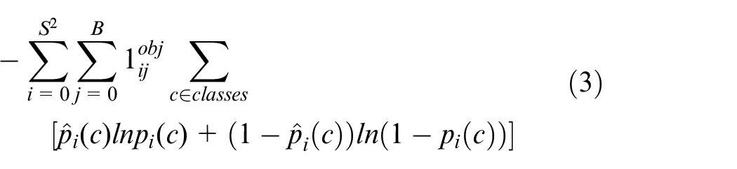
where
Through the above loss function, the gradient is calculated using stochastic gradient descent to update the network parameters and achieve end-to-end training. In summary, YOLOv3 achieves a good balance between speed and accuracy; however, the experiment results on the MS COCO dataset indicate that YOLOv3 performs poorly with medium and large objects, and the performance of mAP@0.75 is slightly inferior to other models.
Improvement and training process
Because the accuracy of the bounding box containing the object is the main focus, which means whether IoU is good enough. If the IoU is used as a coordinate loss function, it is modified to 1−IoU. However, the IoU has the advantage of scale invariance, which means that the similarity between two arbitrary shapes is independent of their size; the IoU though has the following drawback. First, if there is no overlap between the prediction and ground truth bounding boxes, the IoU is 0, which cannot reflect if two boxes are near each other or away from each other and does not provide any gradient for backpropagation, as shown in Figure 2(a). Second, in the case of the same IoU, the IoU does not reflect the manner in which two objects overlap, as shown in Figure 2(b)
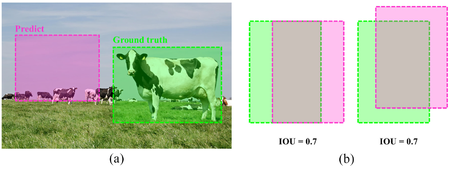
(a) Drawback of the IoU. (b) representation of IOU=0.7.
Owing to the above shortcomings, a Generalized Intersection over Union (GIoU) 22 was proposed by Rezatofighi et al.; the GIoU loss is defined as follows:
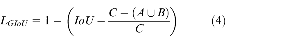
where
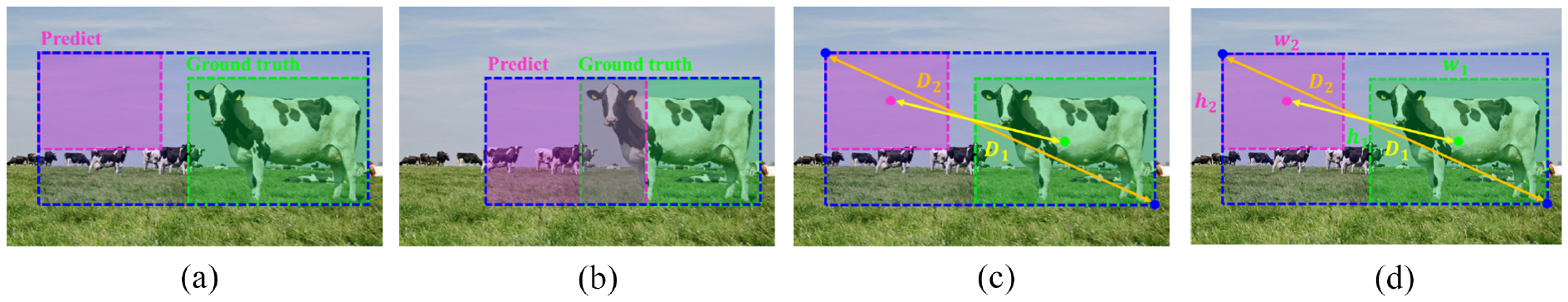
(a) Representation of the GIoU, (b) drawback of the GIoU, (c) representation of the DIoU, and (d) drawback of the CIoU.
Based on the concept of the GIoU, Zheng et al.
23
proposed the Distance Intersection over Union (DIoU) and showed that the GIoU has some shortcomings. When
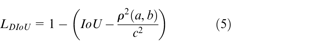
where a and
where
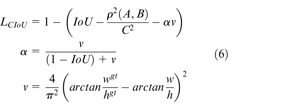
To make the model more robust, we employed two data augmentation methods during training. The first one is Mixup, 24 which multiplies two images and superimposes them with different coefficient ratios to increase image semantics and prevent overfitting, as shown in Figure 4(b). The other method is Mosaic, 25 which randomly crops an area of four images and stitches them into one image, as shown in Figure 4(c). This method mixes four training images, whereas Mixup only mixes two input images. The image semantics achieved with Mosaic are richer than those achieved with Mixup. However, using the four-image mosaic instead of a single image during training reduces the need for large batches.
(a) Original samples, (b) result of Mixup, and (c) result of Mosaic.
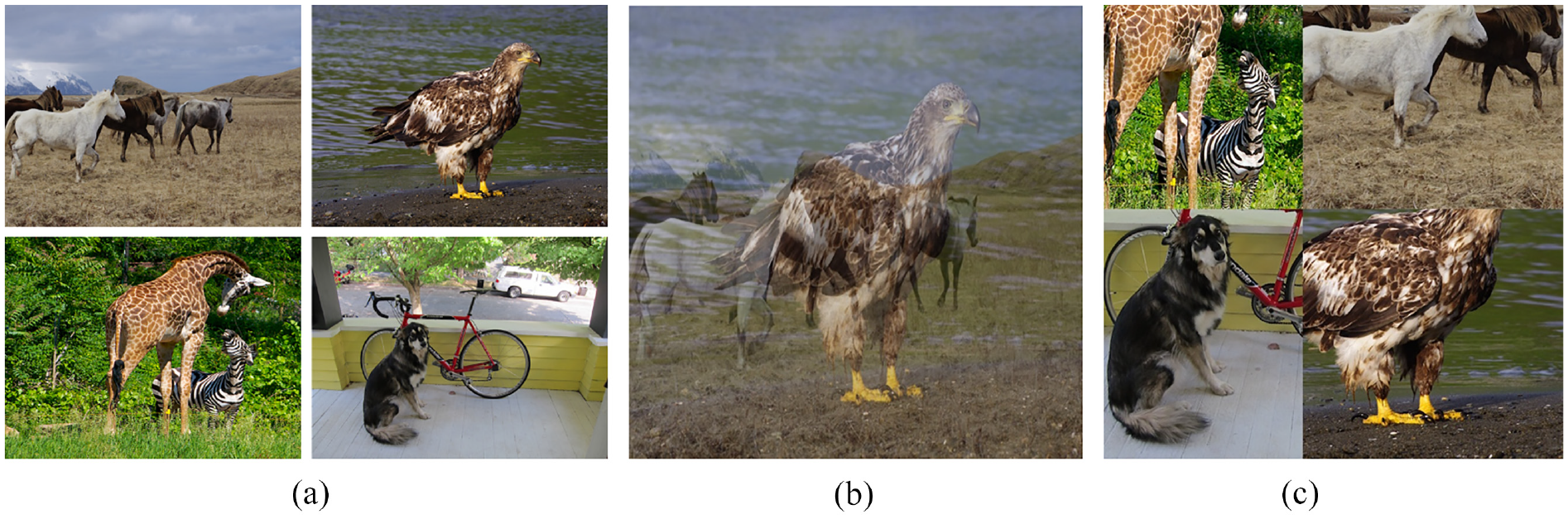
Faces are long, thin, and rectangular. To maintain the original aspect ratio during the image resizing process, the letterbox resize method is adopted; this method prevents the deformation of an object, as shown in Figure 5(c).
(a) Original sample, (b) sample resized without maintaining the aspect ratio, and (c) sample resized with the aspect ratio maintained (letterbox).
In YOLOv3, k-means clustering is used to obtain good priors, which allows the network to learn easily and achieve high detection accuracy. In this study, we also chose nine anchor boxes just like in a previous study 16 ; we applied k-means clustering to our custom dataset. On our custom dataset, the nine clusters were (14 × 19), (19 × 29), (29 × 41), (47 × 46), (39 × 67), (63 × 66), (60 × 109), (93 × 87), and (118 × 109). As seen in Figure 6, most of the boxes were tall and thin, just like human faces. Furthermore, to increase accuracy, we used multiple anchor boxes for a single ground truth instead of a signal anchor box for a single ground truth during training.
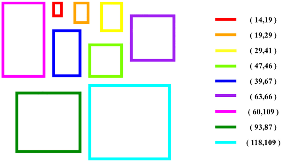
Clustering box dimensions on own custom dataset.
The dataset used in this study consisted of 700 face images collected by us; 750 bounding boxes were manually labeled in three categories. To ensure even distribution of data, we ensured that the number of bounding boxes in each category was equal. Because the amount of training data was less, we used random scaling, cropping, and flipping to prevent overfitting during the training process. In addition, we used the Darknet-53 pretraining model weights that were trained on ImageNet as the initial weights for training to ensure stability during the training process and achieve fast convergence.
System realization and integration
Hardware architecture
The development kit used in this study was Nvidia Jetson Nano. Jetson Nano is a small, powerful computer that is based on a Maxwell architecture with 128 NVIDIA CUDA cores and delivers a computing performance of 472 GFLOPS; moreover, the development boards contain a 40-pin GPIO header. All these features rendered the Jetson Nano suitable for our task.
The mobile vehicle used in this study was a Mecanum wheel. Each wheel consisted of many subwheels arranged at a 45° angle around the wheel axis, as shown in Figure 7(a). The direction of rotation and the speed of each wheel allow the vehicle to move omnidirectionally and attain a higher number of degrees of freedom during operation, as shown in Figure 7(b).
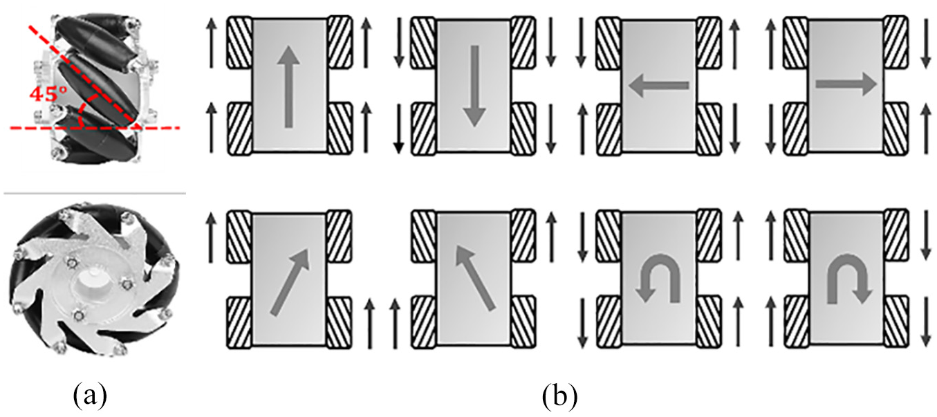
(a) Structure of the Mecanum wheel and (b) omnidirectional movement of Mecanum wheel robot.
Each Mecanum wheel was driven by a JGB37-520 brushed DC motor with a Hall sensor and had a TB6612FNG dual motor driver to control the motor. During movement, the current motor speed was calculated using the signal from the Hall sensor, and the speed information was used for movement control.
For frame capturing, a Logitech C310 webcam was used. This webcam captures images with 1280 × 720 pixels and records videos in 720 p. A gimbal, which consisted of an MG90S servomotor installed to the webcam, and a PCA9850 servomotor driver, which was used to control the servomotor, were used for face tracking.
Because the Mecanum wheel robot is sensitive to the torque of the wheel, it may slip owing to the difference in the motor speed during movement. To prevent slipping, we installed an MPU6050 gyroscope on the vehicle and used Arduino Due to receive yaw angle information through an
The power system consisted of a 5in1 V3 power hub and a 12 V four-cell LiPo battery. The power hub had a linear regulator function to keep the output power stable and provided output voltages of 12 and 5 V to the motor drivers, Jetson Nano, Arduino Due, and other hardware devices. The system is equipped with a low-voltage alarm function to remind users when the battery is about to die to prevent the sudden shut down of the system because of a dead battery.
The Mecanum wheel robot along with the hardware components used in this study is shown in Figure 8; the dimensions of the structure shown in the figure are 26 × 21 × 31 (cm).
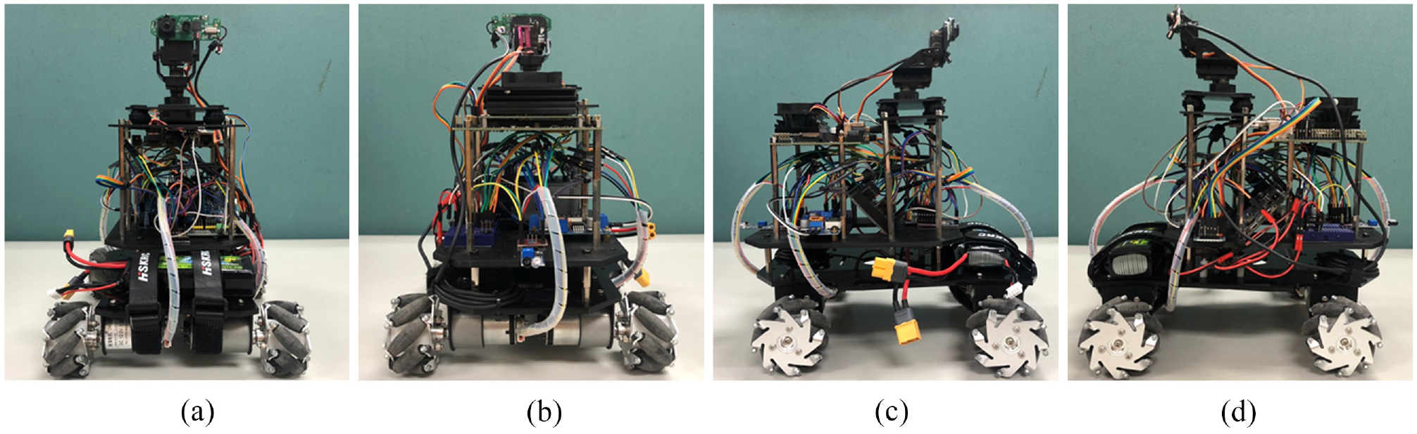
(a) Front, (b) back, (c) right side, and (d) left side of the structure.
Controller design and simulation
To make the system stable and efficient, we need to mathematically model the system before control.26–28 The derivation of the dynamic equations of motion is presented next. The kinematics model of a Mecanum wheel robot is shown in Figure 9.
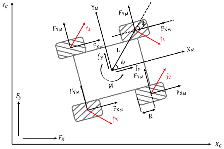
Kinematics model of a Mecanum wheel robot.
Let
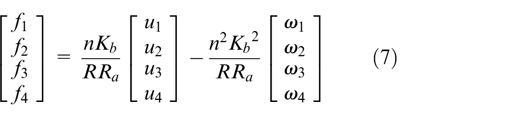
The dynamic equation of motion is
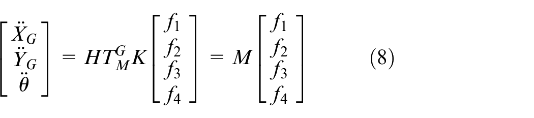
where
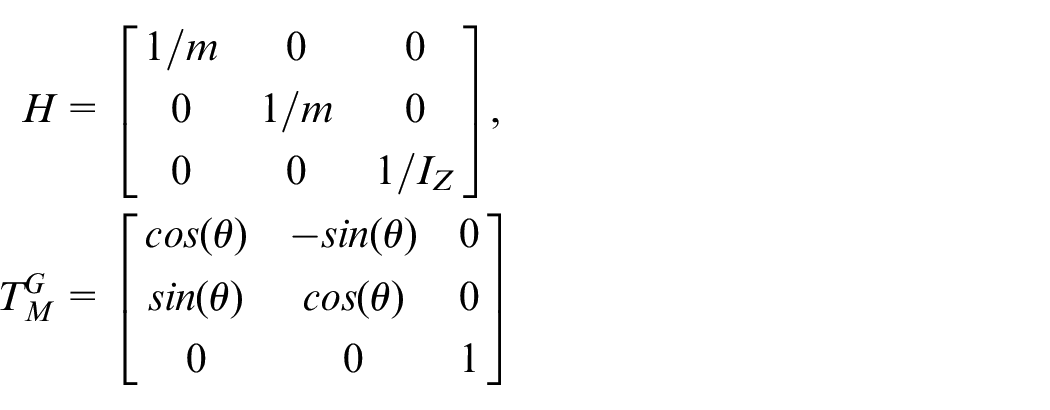
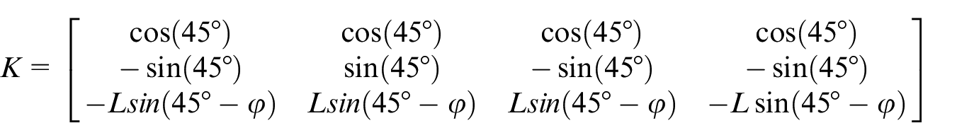
θ is the rotation angle of the vehicle, L is the distance between the vehicle centroid and the wheel centroid, and φ is the angle between the vehicle centroid and the wheel centroid.
The relationship between the velocity of the vehicle and the velocity of wheels is given by :
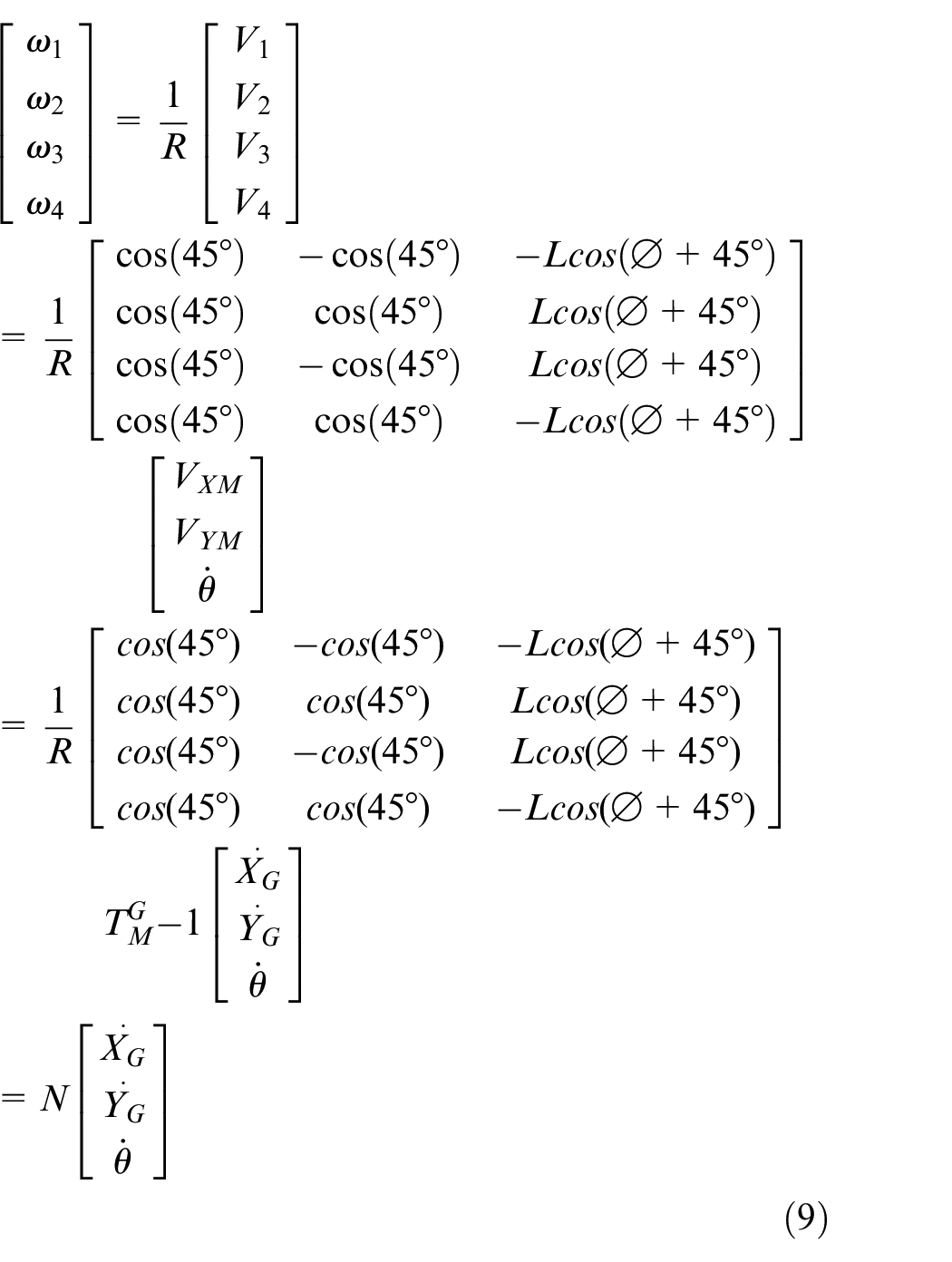
Using equations (7)–(9), the dynamic equations are expressed as follows:
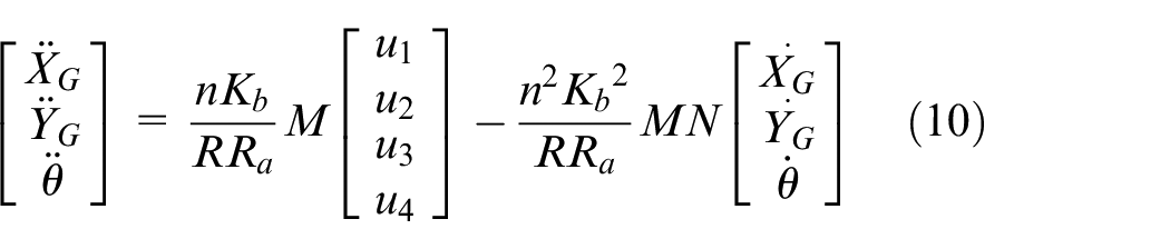
Therefore,
In this study, we use the PID control algorithm to design the controller; A general discrete-time PID controller is represented by :
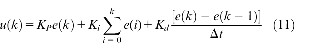
where
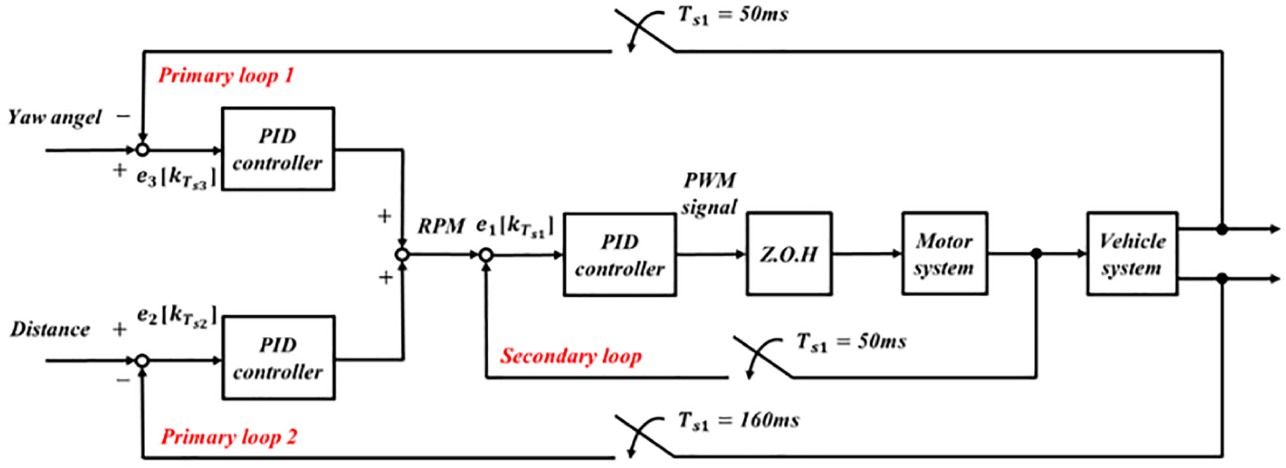
Block diagram of the parallel-cascade PID controller.
First, the secondary loop of the parallel-cascade PID controller is responsible for controlling the motor velocity. The inner loop is executed by Arduino Due, and its sampling time is 50 ms. Each motor has its own PID parameters, that is, there are four sets of PID controllers in the inner loop of the parallel-cascade PID controller. After many experiments and adjustments, the four sets of parameters of the PID controller are as follows:
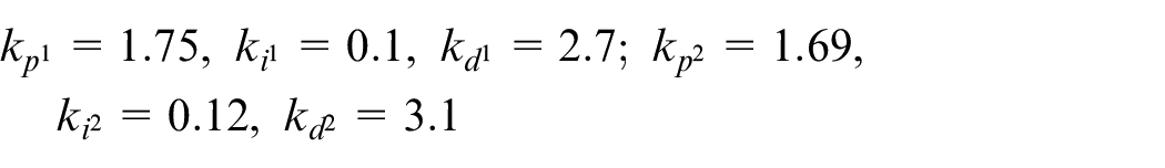
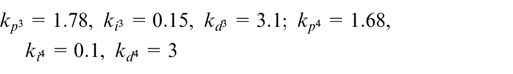
Because the parameters of each motor are slightly different, the parameters of the PID controller for each motor are different. The results of velocity control are shown in Figure 11. The results show that the system has a fast and stable response without any overshoot.
Results of motor velocity control. (a) Result obtained with target RPM of 50, (b) result obtained with target RPM of 100, (c) result obtained with time-variant target RPM, and (d) result obtained with time-variant target RPM.
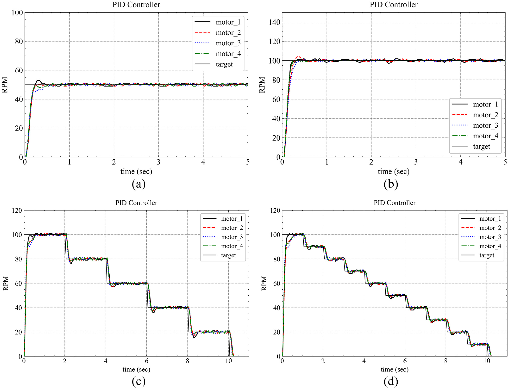
The primary loop 1 loop of the parallel-cascade PID controller is responsible for yaw angle control of the vehicle, which prevents the vehicle from slipping due to the difference in motor speed during movement. The outer loop is also executed by Arduino Due, and its sampling time is 50 ms. The parameters of the PID controller are as follows:

The results of yaw angle control are shown in Figure 12. Figure 12(a) shows the results without the controller. As the vehicle moves, the yaw angle gradually increases, which indicates that the vehicle is slipping, as shown in Figure 12(b). The result after adding the controller is shown in Figure 12(c), the yaw angle is continuously corrected within a range of
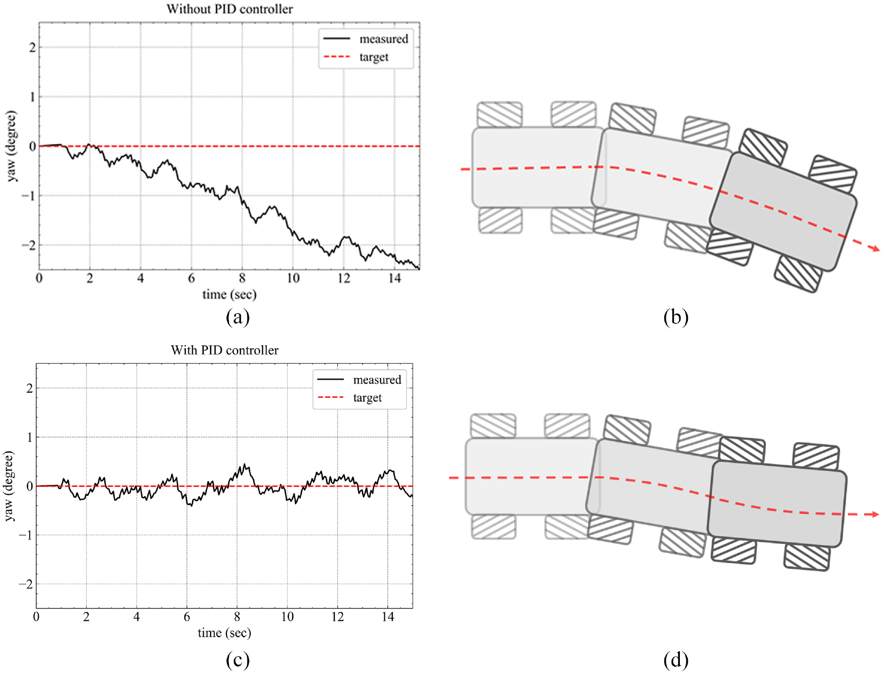
Result of yaw angle control. (a) The result without yaw angle controller, (b) the schematic diagram of vehicle slipping, (c) the result with yaw angle controller, and (d) the schematic diagram of correcting vehicle slipping.
In addition, we provided external disturbances during vehicle movement to test the robustness of the system, as shown in Figure 13(a); and recorded the change of the yaw angle and each motor speed of the vehicle during the process, as shown in Figure 13(c) and (d). According to the result of Figure 13(c), the controller can correct external disturbances immediately, as shown in Figure 13(b). The above test results can prove that the system has good robustness.
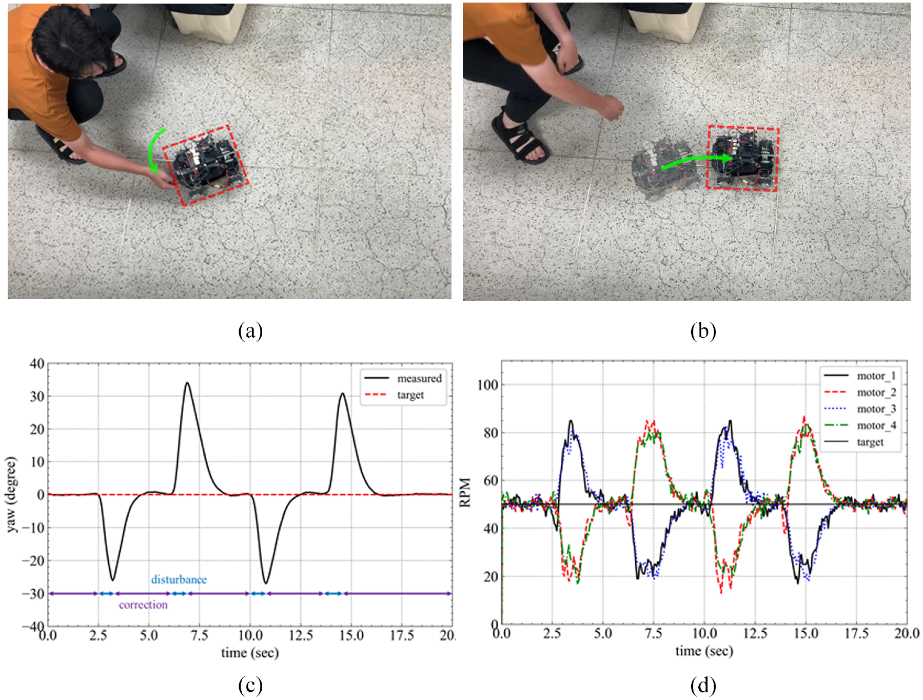
The result of yaw angle control. (a) Provided external disturbances during vehicle movement to make the vehicle slip, (b) actual correction result of the yaw angle controller, (c) the yaw angle of correcting external disturbance, and (d) the RPM of each motor.
The primary loop 2 loop of the parallel-cascade PID controller is responsible for distance control. The outer loop is executed by Jetson Nano, and its sampling time is 160 ms. The distance between an object and the vehicle is calculated using the triangular geometric distance measurement method. 30 The parameters of the PID controller are as follows:

The results of distance control are shown in Figure 14. 150 cm must be maintained between the object and the vehicle. When the object is moving, the vehicle tracks the object through feedback control and maintains a fixed distance from the object. During the movement of the vehicle, the distance between the object and the vehicle is proportional to the vehicle velocity, thereby overcoming the problem of the vehicle being sensitive to the boundary of the target distance.
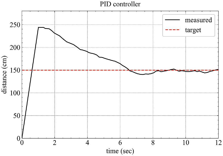
Results of distance control.
Experiment results and discussion
In this study, we used an Nvidia GTX 1080 Ti GPU to train the model through the Darknet framework 31 in an Ubuntu 18.04 environment. During training, we use the SGD with a batch size of 16, the momentum and weight decay are respectively set as 0.95 and 0.005, and adopt batch normalization. The learning rate is set as 0.001 and divide it by 10 at 16 k and 18 k iterations, and terminate training at 20 k iterations. The experimental results are shown in Table 1, all the network input resolution is 288 * 288 except for items with HR, which is 416 * 416. Obviously, a series of optimization methods were used to improve mAP by 8.5% on the custom data set.
In the Table 1, the most significant improvement is the optimization of the coordinate loss function, which uses DIOU loss to replace the mean square error and cross-entropy loss, it confirms that the model cares more about the performance on IoU rather than the scale of the bounding box. The use of K-means anchor Box and Letter-Box resize scheme has increased the mAP by 1.6%, which is optimized for the task, so this effect is predictable. The data argumentation methods of Mixup and Mosaic can make the training data have rich image semantics and avoid overfitting. However, the Mosaic method decreased mAP by 0.6%, we think the reason is that mosaic mixes four input images to make the objects smaller. In addition, human faces are usually small in the images, so that the model cannot handle them. Increasing the data resolution in the training process can make the image information richer, but the relative execution efficiency will be affected, so this is a trade-off that must depend on the task.
Finally, considering execution speed, we selected the result with the highest mAP@.5:.95 at a resolution of 288 × 288 as the face recognition model as shown marked in red in Table 1. The experiment results obtained with the face recognition model are shown in Figure 15(a). The model does not get confused when there are several faces; it accurately determines the location of the object and its category. Figure 15(b) shows the result of real-time detection and distance calculation obtained using the Logitech C310 camera.
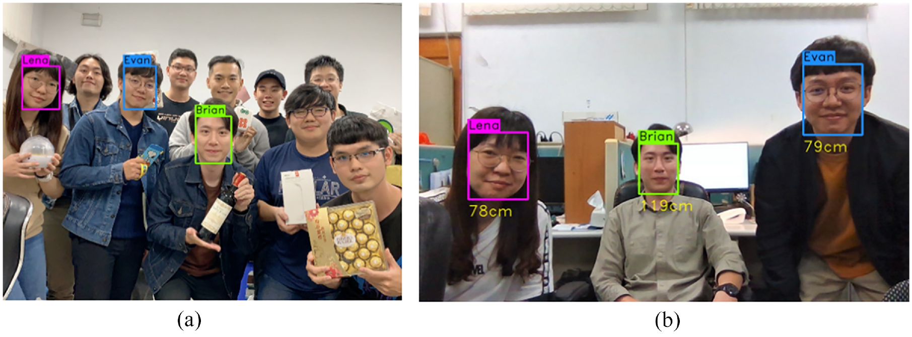
Results of face recognition model. (a) Test result of model and (b) result of real-time detection and distance calculation.
If the face recognition model is inferred on Jetson Nano using OpenCV, 32 its computational efficiency would not be suitable for real-time detection tasks; therefore, we optimized the computational efficiency using TensorRT. 33 TensorRT is a C++ library from NVIDIA; it is used for high-performance inference on NVIDIA GPUs and deep learning accelerators. The inference speed after acceleration is shown in Figure 16. As seen in the figure, the inference speed with TensorRT was more than five times that with OpenCV. Therefore, TensorRT was used to optimize the model, Jetson Nano was used to deploy the model in this study. The use of a more powerful embedded system such as Jetson AGX Xavier can certainly increase computational efficiency but the high cost is contrary to our low-cost purpose.
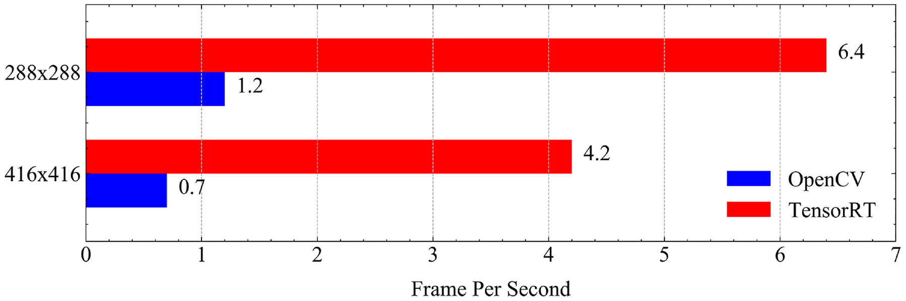
Inference speed comparison of OpenCV and TensorRT on Nvidia Jetson Nano.
To avoid losing the target during the tracking process, we used the PID controller to control the horizontal and vertical rotation of the two-axis servo gimbal, which is shown in Figure 17(a). The pink and blue lines in the frame indicate the horizontal and vertical changes in the target and camera, respectively. When the target moves, the camera follows the target to ensure that the target is in the center of the frame to achieve face tracking. Because three categories are present in our custom dataset, the same effect is achieved by changing the tracking targets, as shown in Figure 17(b).
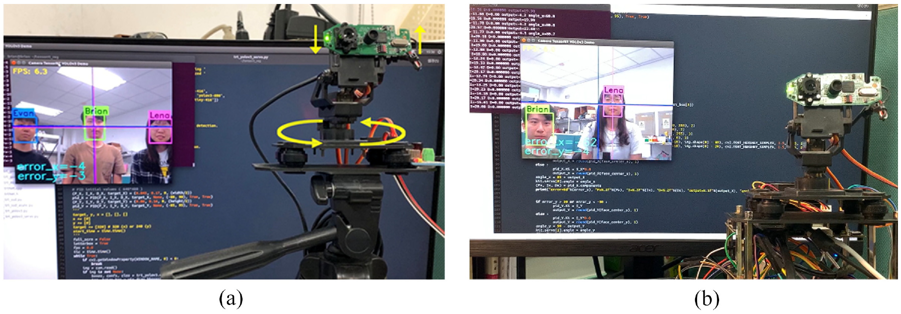
Results of face tracking. (a) Result of face tracking with PID controller and (b) result of face tracking using PID controller for different targets.
The system flowchart is shown in Figure 18. First, the camera inputs the image into the model to determine whether the object exists, after which it calculates the distance between the vehicle and the target as well as the yaw angle of the vehicle. The velocity of each motor is calculated through the outer loop of the parallel-cascade PID controller, and the UART communication protocol is used for data transmission. Finally, the inner loop of the parallel-cascade PID controller controls the velocity of each motor to realize object tracking and slip correction. The other process is to calculate the center coordinates of the target, and then use the PID controller and servomotor to realize face tracking.
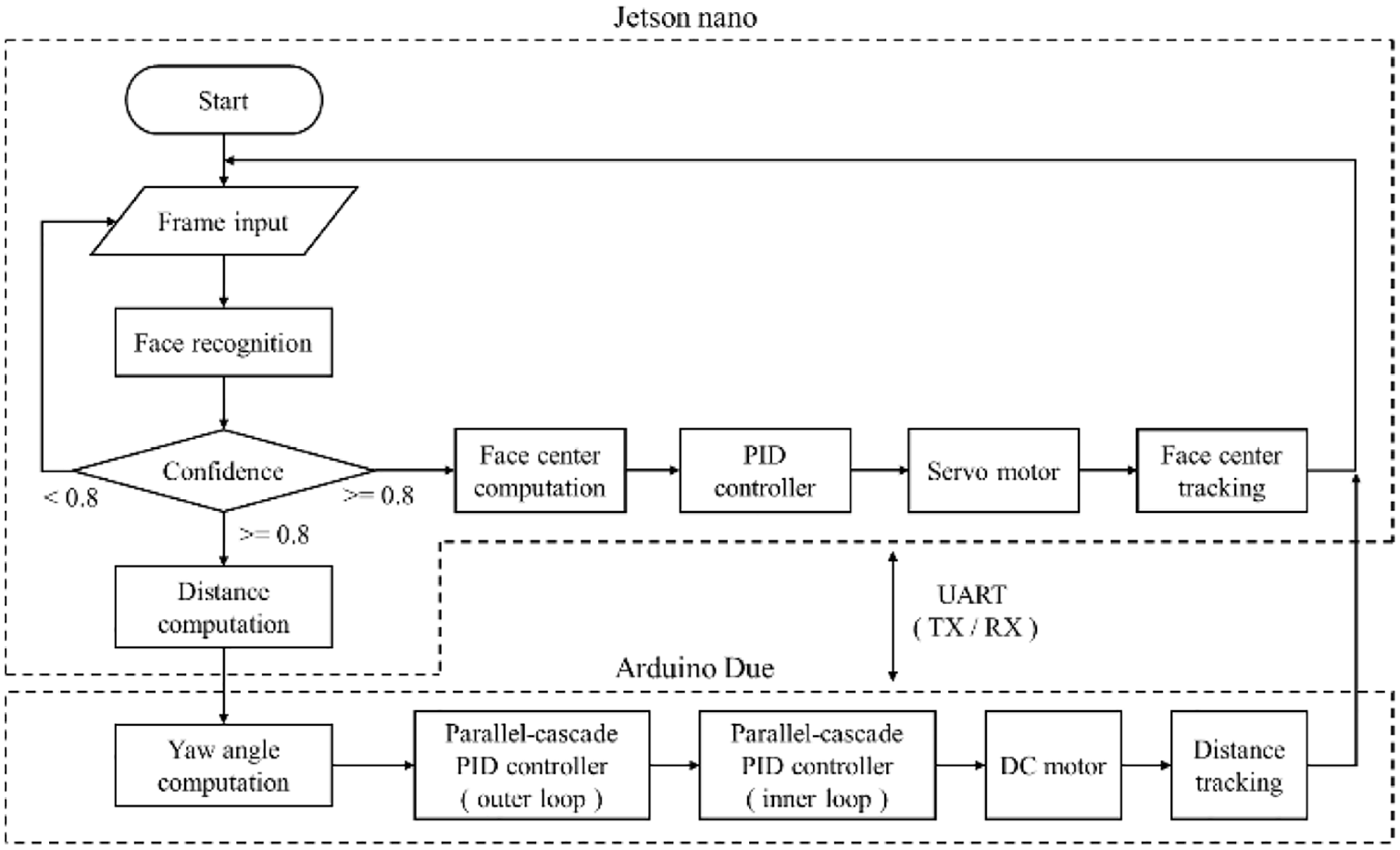
System flowchart.
In summary, the result of the system is shown in Figure 19. As the target moves, the vehicle will adjust the moving speed according to the distance and maintain a fixed distance from the target, and correct the vehicle slip during the tracking process.
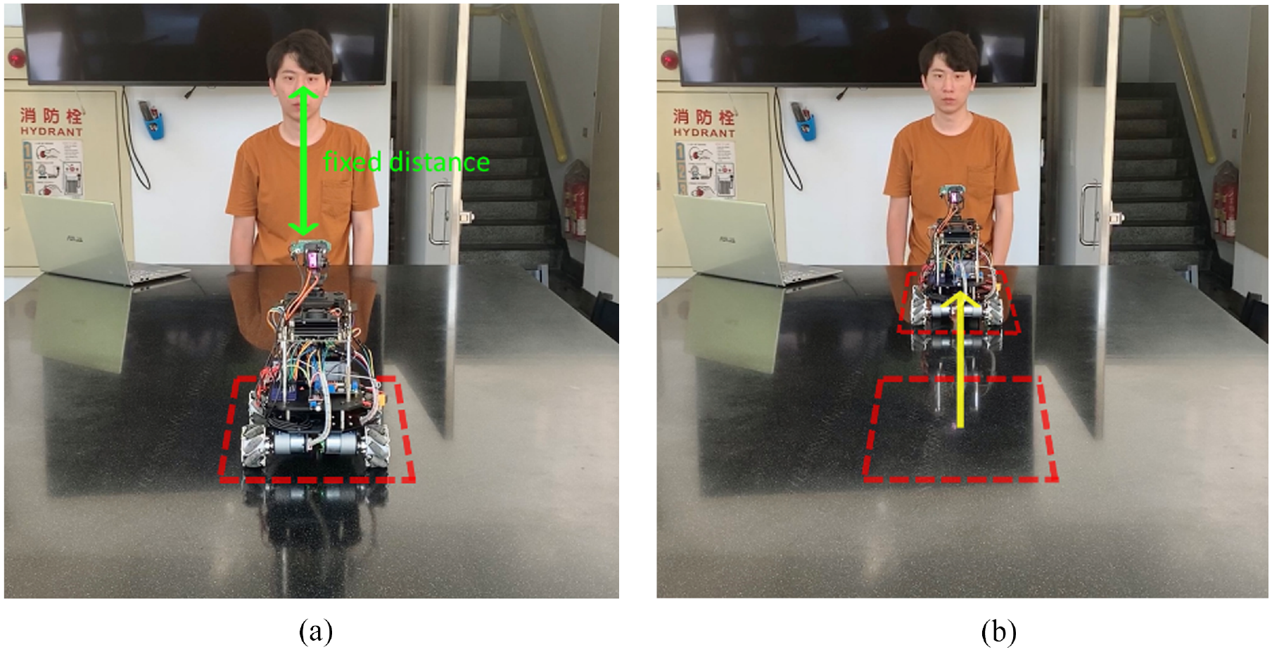
Execution results of system. (a) The actual result of keeping a fixed distance from the object during tracking and (b) tracking demonstration of moving target.
Conclusion and discussion
In this study, we developed an object detection algorithm based on convolutional neural networks. We trained a face recognition model with both accuracy and efficiency using our custom dataset and improved the recognition accuracy through algorithm optimization. We used the concept of edge computing to deploy models on local embedded systems and were able to increase the model inference speed using deep learning accelerators. To increase the stability and robustness of the system, we developed a parallel-cascade PID controller architecture for a Mecanum wheel vehicle. The controller used the distance between the vehicle and the object, the yaw angle, motor speed, and good parameter adjustment to ensure that the vehicle tracked the object from a fixed distance tracking and corrected for vehicle slip during vehicle movement. On the camera, we built a two-dimensional servo gimbal and used feedback control of the PID controller, which allowed the camera to rotate horizontally and vertically, to realize face tracking. Finally, through the integration of software, firmware, and hardware, an omnidirectional unmanned mobile vehicle tracking system with recognition and tracking functions was achieved.
Footnotes
Declaration of conflicting interests
The author(s) declared no potential conflicts of interest with respect to the research, authorship, and/or publication of this article.
Funding
The author(s) disclosed receipt of the following financial support for the research, authorship, and/or publication of this article: This work was financially supported by the Ministry of Science and Technology, Taiwan, under grant MOST 107-2221-E-006-222, MOST 110-2218-E-006-014-MBK and MOST 111-2218-E-006-009-MBK.