
Abstract
This paper presents XXY stage alignment with an image feedback system consisting of two charge-coupled devices (CCDs) and a proportional–integral–derivative (PID) image servo system tuned by particle swarm optimization (PSO). The initial stop values for the PSO algorithm often cause problems in calculation. A long short-term memory (LSTM) deep learning model can identify long-term dependences and sequential model data. Using LSTM to improve the PSO algorithm for searching best fitness value. LSTM predicts the fitness value of PSO, eliminating the need to preassess fitness, value, and uses the predicted fitness value to adjust the inertia weights of PSO adaptively. This allows the PSO search to be terminated in an early stage and reduces the time required for the search. Proposed method was applied to a visual servo system consisting of two CCD cameras and a personal computer–based PID controller for XXY stage motion. The experimental results indicate that LSTM can reduce the time required for PSO fitness search for controlling XXY stage motion under different conditions successfully. Through the training of the LSTM model, the stage positioning error and time of finding optimal control parameters for a coplanar XXY stage can reduced significantly for in-line inspection processes.
Keywords
Introduction
With the rapid development of industrial science and technology, positioning systems have been widely applied in the field of precision manufacturing. 1 With the development of computers, communications, and consumer electronics, high-precision alignment systems have become increasingly crucial to component manufacturing processes, such as the lamination and electrical testing of touch panels – which involve resistance, capacitance, and linearity parameters – electrical testing for open circuits or shorts, the testing of printed circuit boards (PCB), and the manufacture of light-emitting diodes from wafers. 2 When wafer masks are applied, a precision position platform is used to correctly position and orient the panel. Accordingly, accuracy and quality are crucial to the manufacturing process. 1 Many alignment systems now use coplanar stages for high-precision alignment because such stages are faster than stacked ones. This is because coplanar stages have a lower center of gravity and less inertia. 3 Coplanar stages also have higher angular resolution and cost less than direct-drive motor stages. According to kinematic equations, the motors on a coplanar stage can be operated simultaneously to move the stage to the target position faster than a stacked stage can move. 2
Computer vision in has been widely used in image-based technology.4–6 Vision systems function like the human eye, which can automatically detect and recognize images. Therefore, this study’s proposed platform control uses computer vision for image detection and the processing of image signals. Image-processing technology can improve the accuracy of stage positioning and the effectiveness of stage control methods. 1
Kim used two CCD cameras, an XYθ stage, and a feed-forward neural network controller for alignment in wafer manufacturing. The positioning precision was approximately 1 pixel (approximately 12 μm). The alignment performance was approximately 6% superior to that achieved with conventional algorithms. Kim et al. 7 employed a cross mark for alignment. Cross marks are commonly used in many visual alignment systems because they have clear features and can be easily identified. Huang and Lin 8 used a CCD camera, a stacked XY stage, and cross marks for alignment. A fuzzy logic controller was used to control the motion of the alignment stage, and the imaging software eVision was used for image processing. The steady-state error was less than 1 μm.
Alignment using stacked XYθz stages usually causes cumulative errors, such as parallelism errors, orthogonal errors between axes, and flatness errors. Tarng and Lin9,10 used Coplanar XYθz stages have been used to avoid such errors, and they have exhibited superior positioning accuracy to that of stacked stages. Lee and Liu 11 presented an image alignment system with visual servo control that used a specially designed coplanar XXY stage, and each alignment motion was completed in less than 1 s, with an precision of ±1 μm and ±5″. Lee et al. 12 proposed a system consisting of four CCDs, two alignment objects, and a specially designed parallel stage with three degrees of freedom. The alignment displacements for the the X-axis, the Y-axis, and the angle of the rotation, were analyzed through forward kinematic analysis. The linear and angular positioning repeatability of the XXY stage was better than 1 μm and 20″. The alignment error was approximately ±1 pixel. Yang et al. 13 proposed automatic locating and image servo alignment for the touch panels of an automatic laminating machine; the design employs four CCD cameras integrated with a coplanar XXY stage. Lin et al. 14 designed an optical alignment system using a coplanar XXY stage integrated with dual CCD cameras and used a neural network–based method to increase the accuracy of their image servo system. However, the time required for image pattern matching and image processing should be reduced for real-world applications. Lin et al. 15 used a microcontroller for an image-based XXY positioning platform. By incorporating image recognition technology, they could detect the position error between XXY and a detected object. Such error information can be used for positioning control. 1
Conventional proportional–integral–derivative (PID) controllers are widely applied in control systems for their practicality and robustness. PID gains must be properly tuned to ensure superior dynamic performance, security, and the sustainability of equipment and plants. 16 Several approaches have been used to determine the parameters for PID controllers, including the Ziegler–Nichols tuning formula (for time response), frequency domain shaping, genetic algorithms (GAs), 17 and Moth Fly Optimization (MFO). 18 The performance of a PID controller designed using these techniques is satisfactory but may be suboptimal because any constraints on settling time, overshoot, or undershoot and disturbances are system dependent. Kennedy and Eberhart 19 introduced particle swarm optimization (PSO) in 1995. PSO simulates simplified social behavior and can efficiently solve continuous nonlinear optimization problems. As a swarm intelligence technique, PSO is one of the population-based optimization algorithms. PSO is attractive for several reasons. First, the PSO algorithm requires only a few lines of computer code. Second, its search technique is simple and uses the fitness value of the objective function instead of gradient information. Third, it is computationally inexpensive because its memory and processing speed requirements are low. Fourth, unlike conventional deterministic methods, PSO does not require strong assumptions about linearity, differentiability, convexity, separability, and can work under constraints to solve problems efficiently. Finally, its solutions do not depend on the initial states of particles, which represents an advantage for design optimization problems in engineering.20–22
Therefore, accurate real-time historical mapping of the relationship between the parameter fields of the controller and the integral of the absolute magnitude of error (IAE) is necessary. One deep learning model, the long short-term memory (LSTM) network, is highly proficient in time series forecasting in various fields because it can dynamically learn new information while retaining a consistent memory of historical information. Sagheer and Kotb 23 performed time series forecasting for petroleum production by using recurrent LSTM networks optimized by a GA. The LSTM model outperformed other standard approaches. Zhang et al. 24 employed an LSTM network to predict the remaining useful life of lithium-ion batteries. Zhang et al. 25 developed an LSTM model to predict water table depth in agricultural areas and evaluated the abilities of the proposed model. The LSTM model achieved satisfactory performance. Qin et al. 26 employed an LSTM model to predict the remaining life of gears. LSTM networks can capture both short-term correlation and long-term dependence. Gao et al. 27 employed the thermal error model by using LSTM networks which was optimized by PSO, the PSO-LSTM model is established to precisely predict the thermal error of ball screws, and then provide a foundation for thermal error compensation. Qiu et al. 28 performed a railway freight volume forecasting model by using LSTM networks optimized by PSO, and then the PSO-LSTM model has lower prediction error and higher prediction accuracy than the traditional LSTM and model GA-LSTM. However, few studies have investigated using LSTM networks to predict the IAE of machine controllers, especially for XXY stages.
This study attempted to overcome three main challenges of image servo mask alignment system using an XXY stage through intelligent machine tuning. The first challenge is solving the problem for the lack of linear scale for displacement measurement and the nonlinear positioning error due to mechanical accuracy of the nonlinear motion of the stage. Although coplanar XXY stages have some advantages, such as lower cumulative error and quicker responses, than stacked XYθz stages, motion planning for XXY stages is difficult because the individual movement along the X1-axis, X2-axis, and Y-axis is coupled with the others, and their kinematic relationship is nonlinear. Therefore, this study developed an image-based method to solve this problem. The second challenge is that the lack precision caused by the semi-closed loop control of the servo motor. This study proposes a PID control for visual servo control system based on PSO tuning controller parameters. The third challenge is predicting the fast convergence fitness value for PSO algorithm. Since the stop bettering fitness value for stop PSO computation must be obtained experimentally, but this may cause time consuming; therefore, this study uses the characteristics of LSTM to predict the fitness value for PSO and stop the PSO algorithm after fewer iterations. The fourth future challenge is the assembly of a precision stage demands time for fine tune of individual control parameters. Knowing the machine positioning accuracy is a key priority. Since the remaining useful life of motion stage could decay after long time operation. As for prognostic health maintenance issue, PSO-LSTM model can be deployed in shop floor system.
This paper is organized as follows: in Section 2, experimental setup including hardware of XXY stage, vision system and controller; in section 3, fundamental of PSO; in section 4, LSTM network; in section 5, the XXY stage motion with PSO–LSTM model; in section 6, experimental analysis; and in section 7, contributions are concluded.
XXY system principle and structure
XXY stage hardware
The XXY stage is characterized by three motors on the same plane with the merits of low gravity center. In other words, the moving speed of XXY stage can be faster than the traditional stacked XYθ stage. It is small and light. Thus, the main advantage of XXY stage is being smaller cumulative error of stage composition than the traditional stacked stage. Therefore, the coplanar XXY stage are very popular for the applications of precision motion, such as AOI and lithography. 15
As shown in Figure 1, the system hardware consists of the upper mask chip device, which carries the upper cross mask for CCD’s imaging, the lower coplanar XXY stage (XXY-25-7, CHIUAN YAN Ltd., Changhua, Taiwan), 29 which carries the lower part to align the upper device with the image servo control, and two CCD camera lens, which are mounted on the top of the system as the image servo sensors for positioning. A motion card (PCI-8143, ADLINK TECHNOLOGY INC, Taiwan) control the XXY stage, 30 and ADLINK’s Domino Alpha2 image card was used for XXY stage image position feedback. Picture of the XXY experimental stage was shown in Figure 2.
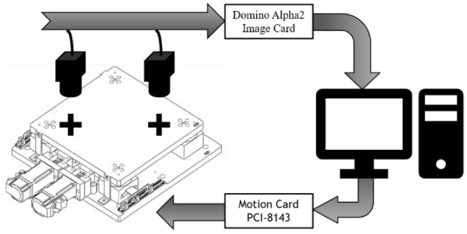
Configuration of XXY stage system.
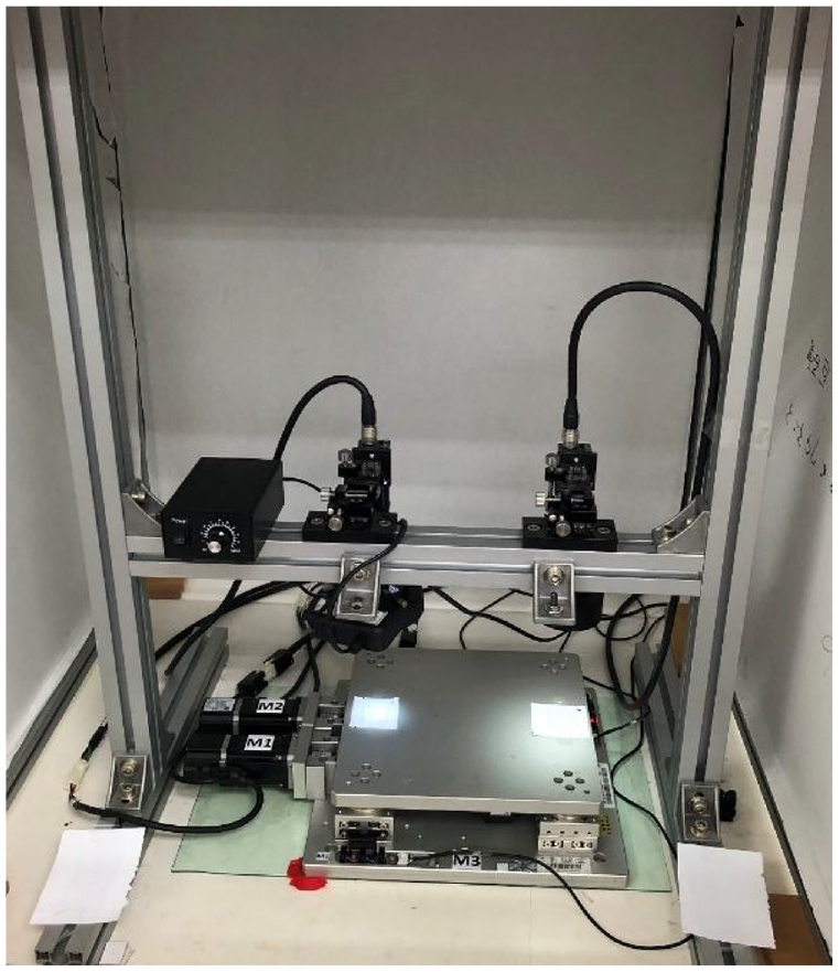
Picture of the XXY experimental stage.
Traditional XYθ stages use the stacked design, which consists of an X-axis translation stage, a Y-axis translation stage, and a θ-axis rotational stage. The controller design for traditional stacked XYθ stage is simple because the movement of each axis is independent. However, the XYθ stage produces cumulative flatness errors due to the stacked assembly and the large size of the stage. Therefore, coplanar XXY stage was developed because the coplanar design produces lower cumulative error and can move faster than the traditional XYθ stage. Figure 3 displays the structure of the coplanar XXY stage, which is driven by three servo motors, the X1-axis motor, X2-axis motor, and Y-axis motor. The working stage is supported by four substages; each substage consists of X translation, Y translation, and θ rotation stages. Therefore, the motion of the XXY stage has three degrees of freedom: the translation along the X-axis and Y-axis and rotation around the θ-axis.11,15
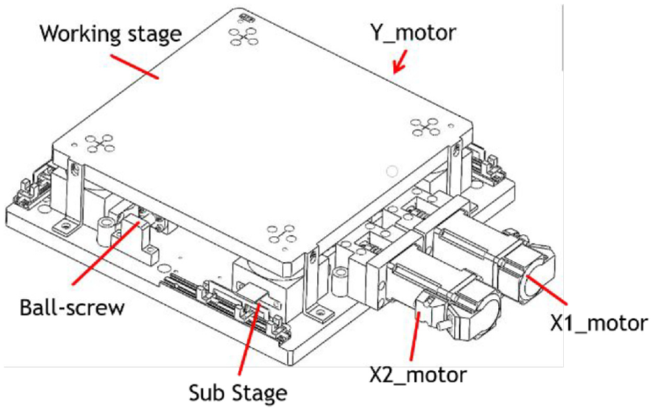
Coplanar XXY stage. 29
The XXY stage can move up to ±5 mm, and the maximal angle is ±2°. When the motors of the X1- and X2-axes rotate clockwise or counter-clockwise and the motor of the Y-axis is static, the stage can move along the X-axis. By contrast, the motor of the Y-axis is used to control the movement of the stage along the Y-axis.
The XXY stage has motion in three dimensions, X, Y, and θ (Figure 4). If the linear displacement of the stage is represented as
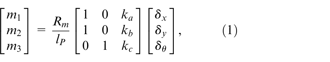
where
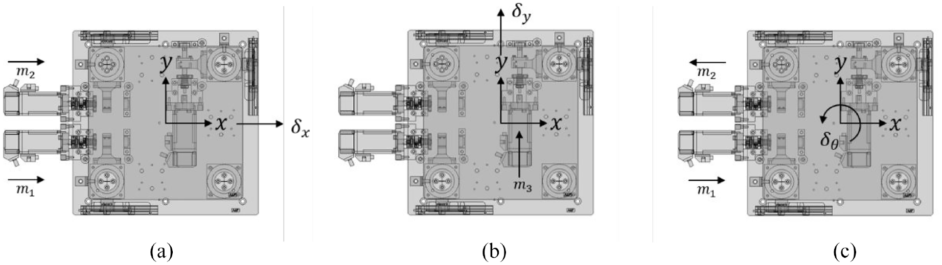
Three-dimensional motion: (a) X motion, (b) Y motion, and (c) θ motion. 28
Vision for XXY stage
The purpose of the proposed image processing method is to determine the position of the alignment symbol through the center of gravity method.14,32 Then, the coordinates of the XXY stage are calculated on the basis of the coordinates of the mask target. Locating the target mark and determining the corresponding relationship between stage movements is crucial tasks. Our method employs the image preprocessing tools.6,7 Binarization and morphology are used to simplify the image and reduce the noise. The preprocessing reduces the residual noise in the image, allowing the features to be separated. Next, the feature coordinates are detected through a simple center of gravity method, and the position of the feature center is acquired.
The center of gravity method is used to obtain the target position in the image coordinate system. Two gray pictures are acquired from the two CCDs. The noise in the images is processed using a filter, and the binary threshold of the grayscale histograms is used to separate the two targets. Expansion and subtraction are used to remove the remaining noise, allowing the optimal image to be identified through a morphological process. Then, feature targets are identified through the findContours function of OpenCV. The center of gravity method is thus used to obtain the coordinates of the center of the image for the positioning mark. Figure 5 displays a flowchart of the image identification procedure, Figure 6 displays the cross mask position results by center of gravity method.
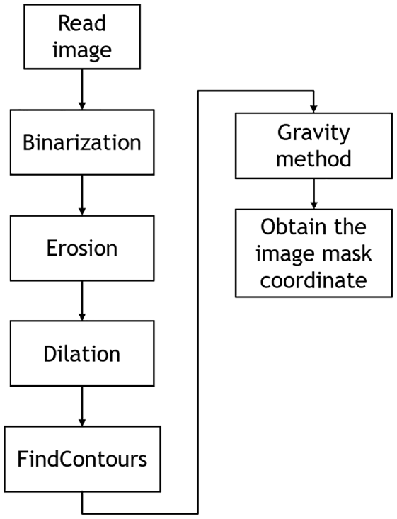
Image identification procedure.
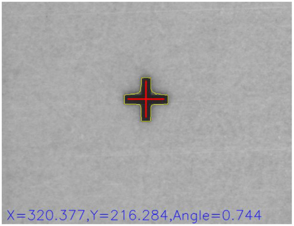
Picture of the cross mask position results by center of gravity method.
Controller for XXY stage
The time domain of the PID controller for the XXY stage is given as follows:
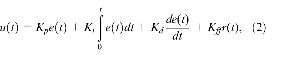
in which r(t), e(t), u(t), Kp, Ki, Kd, and Kff represent input command, system error, control variable, proportional gain, integral gain, derivative gain, and velocity feed-forward gain, respectively. Figure 7 presents the control architecture of PCI-8143 motion card. Each coefficient of the PID controller affects the system’s output response. Therefore, selecting the appropriate gains is crucial for the practical application of this controller. 30
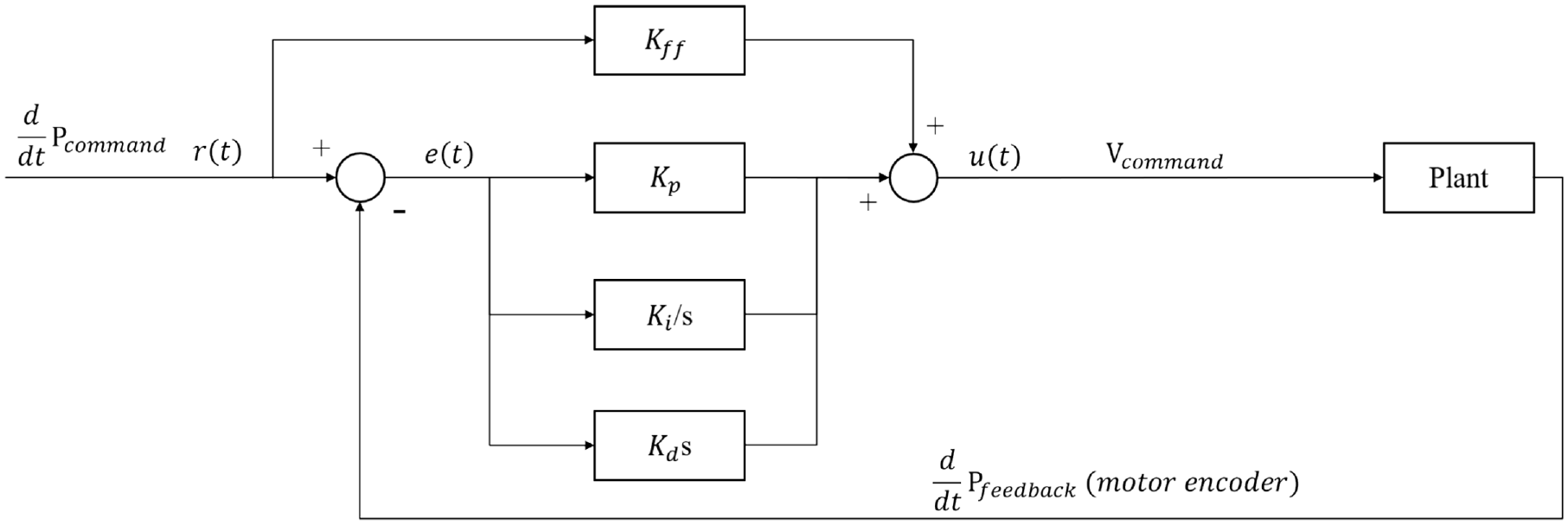
Architecture of PCI-8143 motion card control. 30
Particle swarm optimization
The PSO algorithm is based on a flock of birds and simulates their behavior in a simplified social system. The individual elements in PSO evolve through cooperation and competition through generations instead of through the application of a genetic operator. Each individual is referred to as a “particle” and treated as a point in a D-dimensional space, representing a potential solution to a problem. Each particle adjusts its velocity, position, and best previous position on the basis of its own experience and the experiences of its neighbors.17,18,20 Inertia weight is used to balance the local and global search functions. Because each particle remembers its worst experience, it can explore the search space effectively to identify the most promising solution region. The PSO algorithm can be presented as follows:
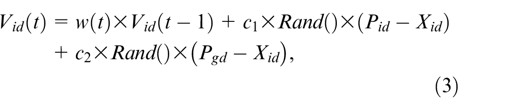

where
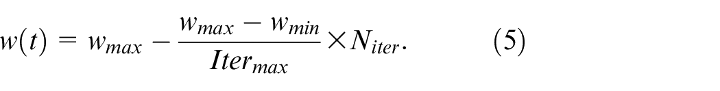
A large inertia weight facilitates a global search, whereas a small inertia weight facilitates a local search. Decreasing the inertia weight over the course of a PSO run enables a greater ability to perform global at the beginning and a greater ability to perform local search near the end of the run. This study set
This study uses PSO and IPSO to tune the parameters of the PID controller. However, the fitness functions must first be established on the basis of a comprehensive evaluation of each particle’s performance. These functions serve as the basis for individual and global particle updating, causing the initial solution to converge toward the optimal solution. This study designed a PID controller with the integral of absolute error (IAE) used for the fitness function. In this experiment, the position of the XXY stage was captured by the CCD, and the capture frequency of the CCD was 30 fps. However, the actual capture frequency is floating, the frequency is about 29–31 fps. Therefore, it is not suitable to use time index to evaluate in the image positioning method. So the integral of time multiplied absolute error (ITAE) and integral of time weighted squared error (ITSE) are not suitable for this experiment, and the trends of IAE and integral of squared error (ISE) are very similar. Each particle constituted with four parameters that are assigned real values for the PID’s proportional gain, integral gain, derivative gain, and velocity feed forward gain, respectively. For n individuals in a population, the dimensions of the population are n× 4. The matrix for a population with a total of 20 particles is as follows:
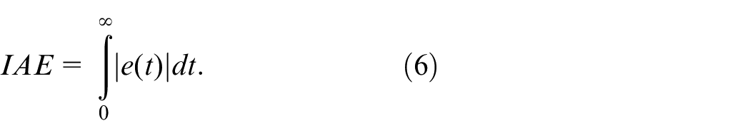
Figure 8 presents a rough summary of the PSO algorithm.
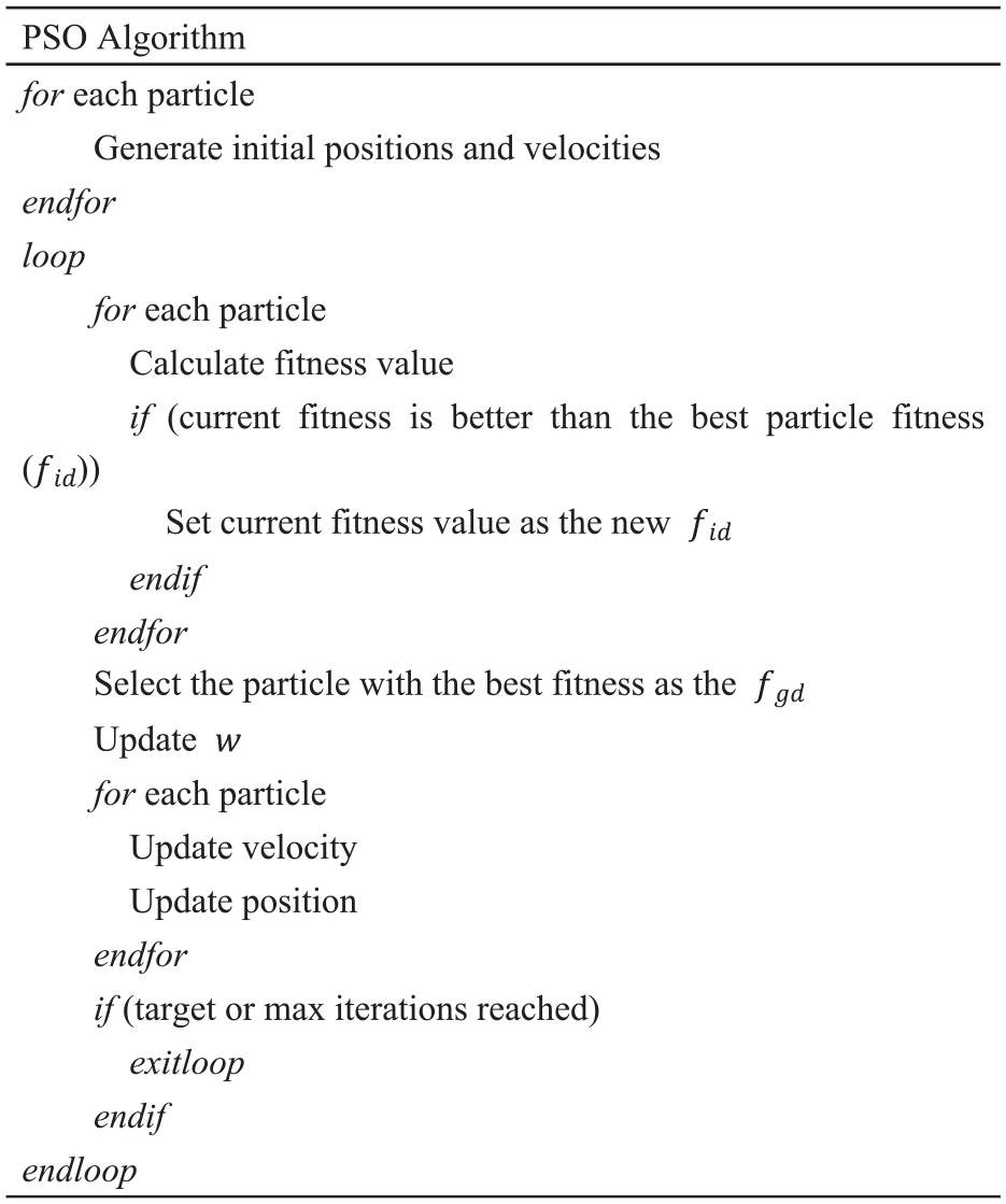
Pseudocode of PSO algorithm.
LSTM network
LSTM is a deep learning model used to solve the problem of gradient vanishing in recurrent neural networks (RNNs).
31
LSTM networks handle nonlinear data effectively, and they are often used for long-term dependencies. Compared with RNNs, LSTM networks use more complex gate structures to process information and storage units to determine which data to forget or retain. Figure 9 presents the internal structure of LSTM. A neuron consisting of an input gate


where
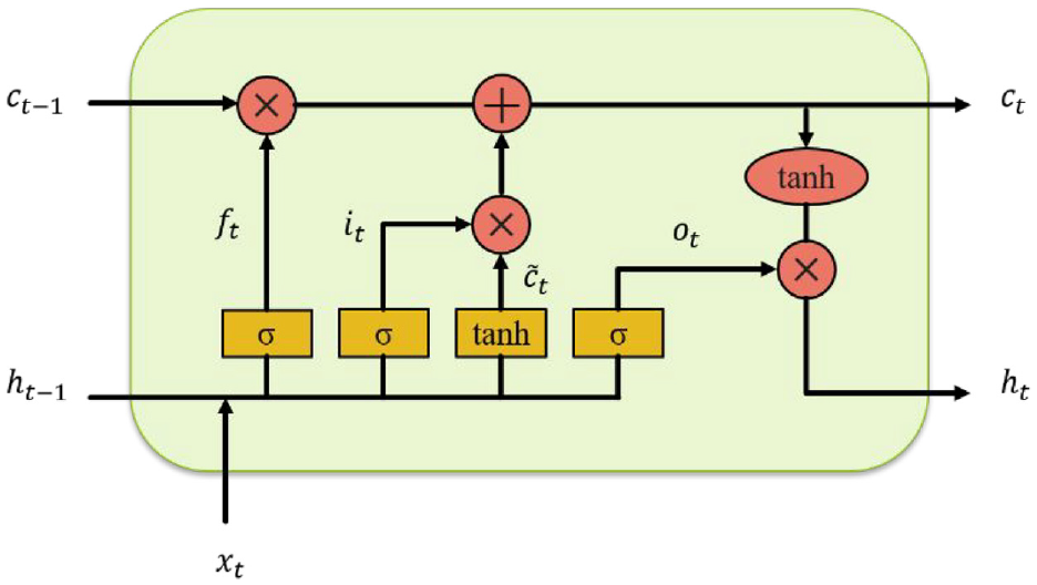
Internal structure of LSTM model.
XXY stage motion based on IAE prediction with PSO–LSTM model
This study uses PSO to determine the XXY stage control parameters. PSO algorithm employs two common stop conditions. The first is a limit on the number of iterations of the search. However, this limit does not result in efficient convergence, but the search time is constant. The second is a target fitness value, but this requires pretesting to obtain a stable convergence of fitness values. Because fitness value differs depending on the stage operating conditions, therefore the dynamic fitness value must be adjusted accordingly.
This study proposes predicting fitness values or trends on the basis of updating controller’s parameters and trained data to determine whether PSO search should be continued or not. This method combines LSTM with the time series structure of neural networks to predict bettering fitness value. The training data input to this LSTM structure consist of the particle position errors from the PSO iteration. The position data consist of the three parameters of the PID controller for the XXY stage, and the output training data was derived from the results of the PSO search for the global optimal particle fitness, then the current PSO particle data is used to predict the current best fitness value of the PSO through the trained LSTM model, as show in Figure 10.
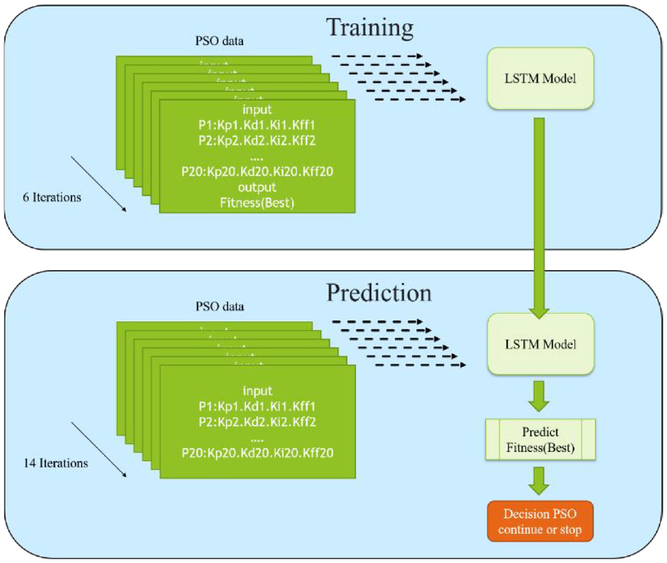
Illustration for the data training and prediction of LSTM model for PSO’s fitness value
PSO search can be continued by predicting fitness value and trends to achieve convergence early to stop the search iteration and avoid being unable to obtain the optimal parameters. When the PSO search is terminated early, computation time is saved.
Figure 11 presents the architecture of the PSO–LSTM model. First, the PSO search data are initialized to generate the position and velocity parameters for the particles. The control parameters of each particle are set in the controller, and then the position of the XXY stage is compensated. Furthermore, the dynamic response displacement of the stage is obtained by the CCDs. The fitness (
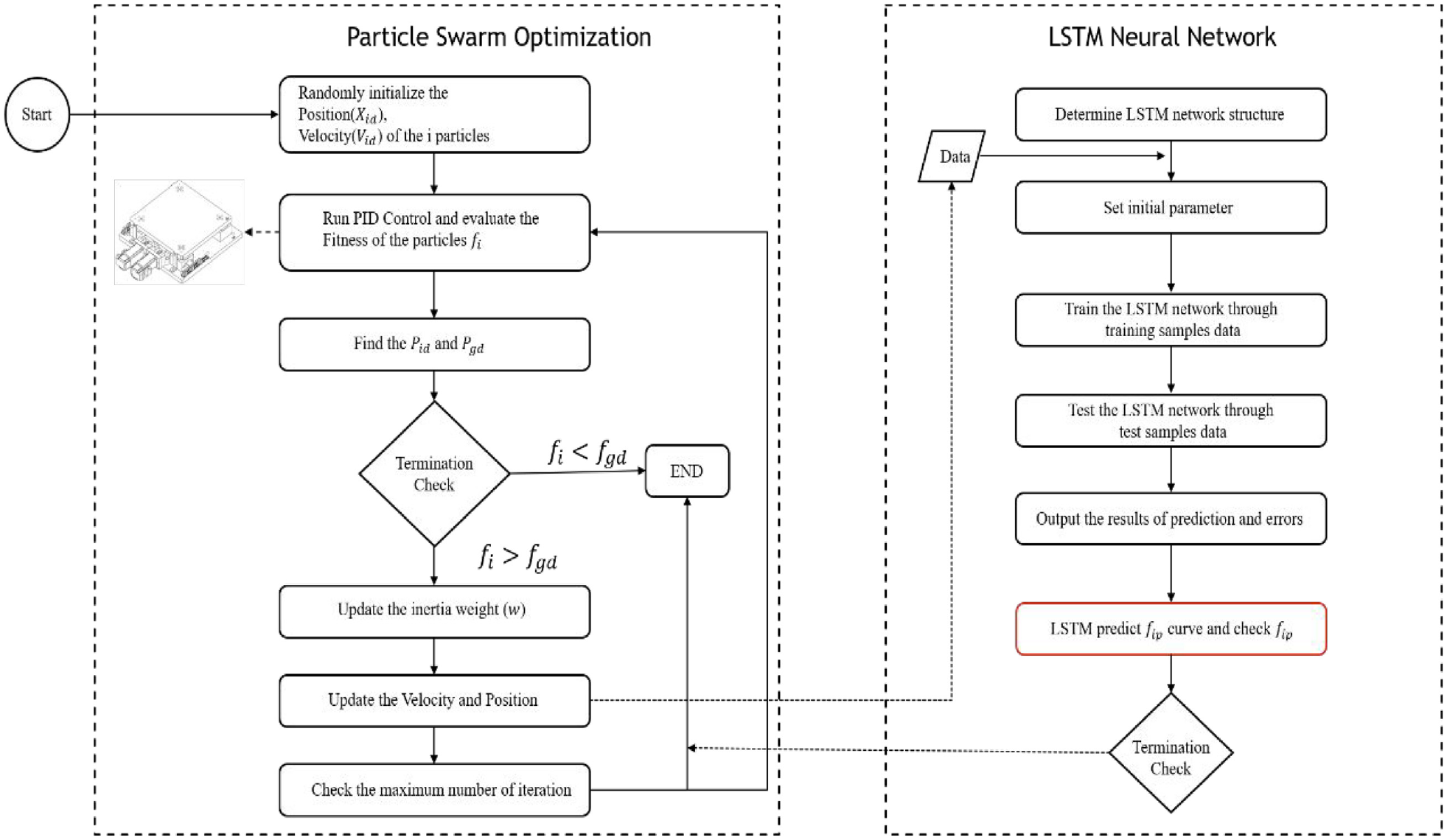
Structure of PSO–LSTM model.
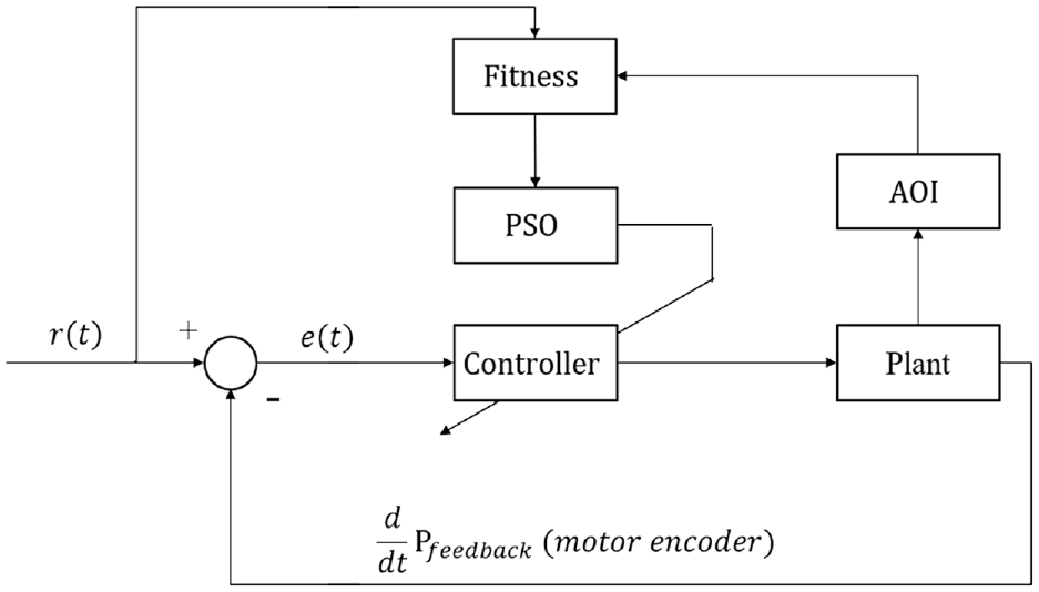
Block diagram of PSO PID closed loop control with automatic optical inspection system.
Experiments
This study used PSO and IPSO to test three types of motion of the XXY stage. The first was single-axis motion in the Y direction. The second was synchronous two-axis motion both in the same X direction, the XXY stage was controlled by two different motors to control the same X-axis direction of the stage motion. The third was three-axis circular rotational motion. The onset of stop PSO’s searching of three experiments was as follows. The particle data of PSO in each iteration were used to predict the current fitness value based on position error through the established LSTM network model, then continue the PSO search, and evaluate or call for stop in advance in comparison with the predicted fitness value from LSTM.
Y-axis experiments
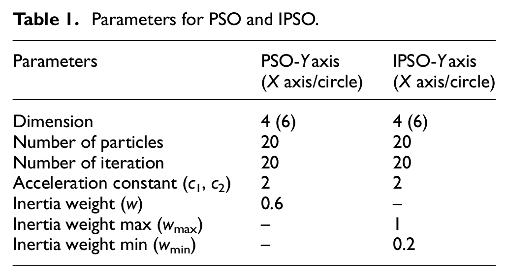
PSO was used to search for the optimal motion control parameters for Y-axis movement of the XXY stage. The motion command was to move 1 mm at a velocity of 1 mm/s. The parameters of the PSO algorithm were as follows: The dimensions were set to 4, representing the four control parameters on the Y-axis, Kp, Ki, Kd, and Kff; the range for the parameters was 0–10,000; the maximal number of iterations was 20; the number of particles was 20; the learning factors (c1 and c2) were set to 2; and the inertia weight w was set to 0.6. For the IPSO experiment, the maximal inertia weight wmax was set to 1, and the minimal inertia weight wmin was set to 0.2. The experiment was terminated when PSO or IPSO reached the maximal number of iterations. Table 1 presents the parameters.
Parameters for PSO and IPSO.
PSO achieved a dynamic motion response that did not reach the target of 1 mm (Figure 13). This may have been caused by mechanism or image error, since the mechanical error of the stage is 20 µm, while the image error is about 1–2 pixels with the resolution of the CCD for 10 µm per pixel. Therefore, theoretically, the total error is about 30–40 µm. With the merit of changing inertia weight at each searching iteration, the IPSO was adaptively to obtain a lower fitness value by reducing w and then strengthen the local search capabilities (Figure 14). Through the adaptive inertial parameter w, IPSO has better adjustment ability than PSO in global search and local search. After 20 iterations, the fitness values obtained through PSO and IPSO were 3.363 and 3.186, respectively. The PSO dynamic response data were as follows: the peak overshoot Mp was 4.88%, the steady-state error Ess was 1.6%, and the settling time Ts and rise time Tr were 0.87 and 0.78 s, respectively. IPSO obtained superior fitness values to those obtained by PSO. For IPSO, Mp was 4.09%, Ess was 2.3%, and Ts and Tr were 0.99 and 1.05 s, respectively. Table 2 presents the data. Although the control parameters were different, the resulting positioning error and dynamics response on the actual platform were pretty similar.
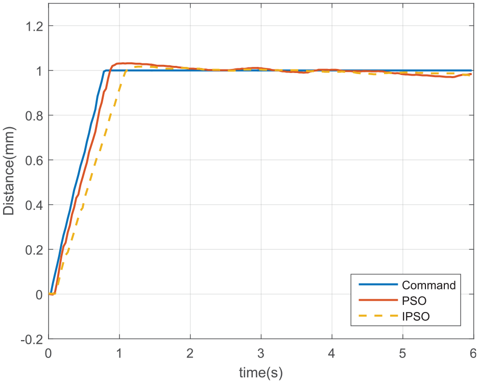
Y-axis step response for PSO and IPSO.
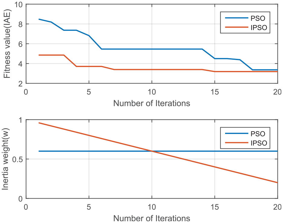
Variation of the fitness and weight value of the PSO and IPSO with number of iteration in Y-axis.
Indices for Y-axis performance of controller tuned by PSO and IPSO.
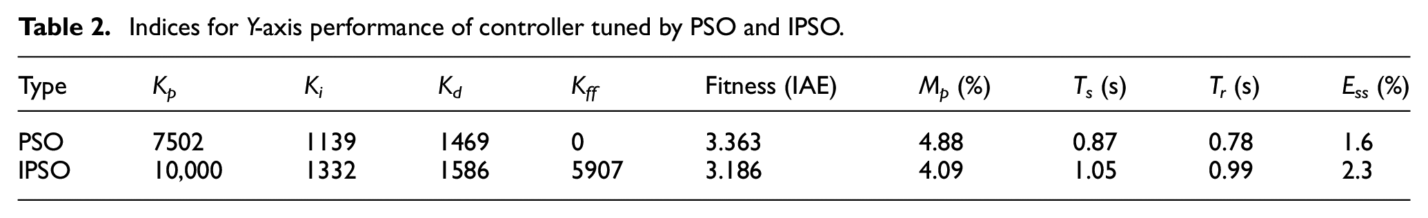
Figure 15 presents a diagram of the particle parameter distributions for PSO and IPSO. PSO exhibited apparently convergence by the seventh iteration (number of iterative particles = 160), and Ki did not converge apparently. This may be because Ki had little effect on the system. IPSO exhibited obvious convergence by the fifth iteration (number of iterative particles = 120) when deploying high w than PSO. Therefore, IPSO exhibits a higher searching ambitious ability at the beginning of the iteration and find lower fitness parameters and fewer iterations in early searching stage. After few iterations, the fitness value in the middle searching iterations is more likely constant. With decreasing w, IPSO can be used to search for optimal control parameters in a conservative way and reach to bettering fitness value more effectively. As a result, the overall dynamic step responses in Figure 13 and the fitness value history in the end of Figure 15(a) and (b) found by the two methods of PSO and IPSO were quite similar.
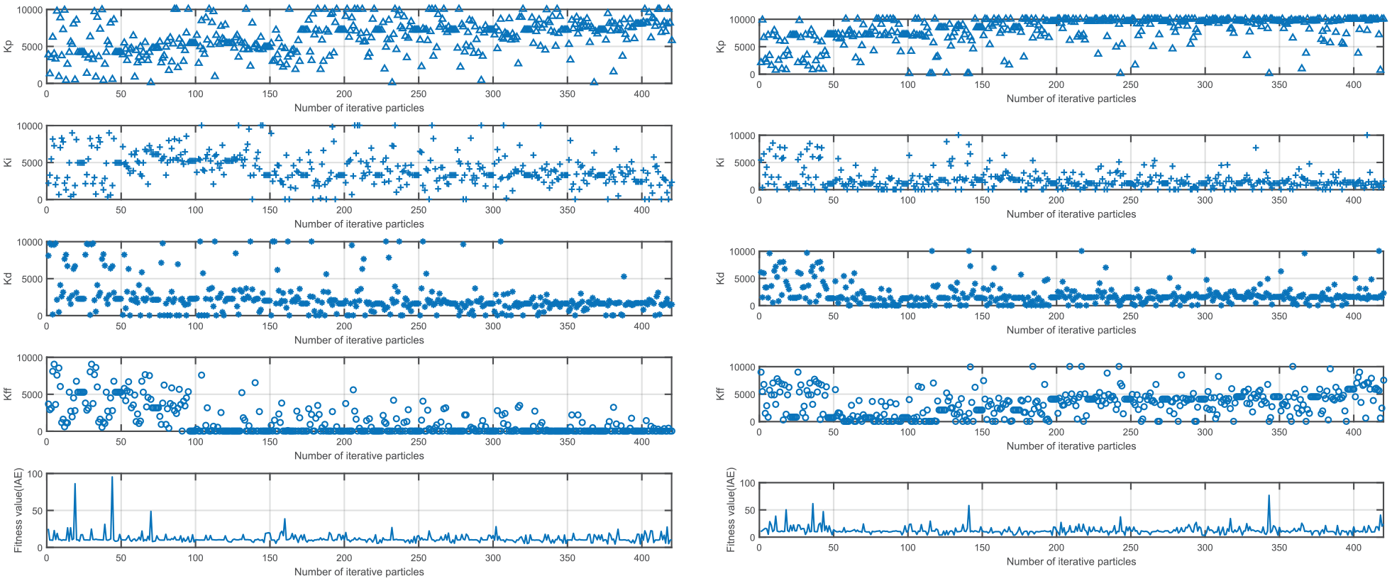
(a) Variation of PID controller gains, feedforward gain, and fitness value with number of iterative PSO’s particles and (b) variation of PID controller gains, feedforward gain, and fitness value with number of iterative IPSO’s particles.
Since the trend of fitness values of the PSO and IPSO differs and depends on initial parameters. The characteristics of time-dependence LSTM was used to find the history of fitness value obtained by PSO and IPSO as repetitive learning (as shown in Figure 11). First, the baseline configuration of the LSTM network was determined by using input and output data, which consisted of particle parameters and fitness values, respectively. Then, fitness was predicted before each iteration of the PSO search. The LSTM model is implemented by using Keras library and contains one LSTM layer and a dense layer.
To train the LSTM model, the weights and biases were updated through Adam optimization. The mean absolute error and accuracy were used as the metrics to evaluate performance. Number of time steps was 6, the input data dimension was 80 (20 particles × 4 control parameters), the number of epochs was 50. The hyperparameters of the LSTM were adjusted using an optimization Adam algorithm because of its ability to quickly find the optimal solution.
As shown in Figure 16, for the first seven PSO searches, the data from the previous PSO search history were input into the LSTM model for training, and then the parameters of the 20 particles were used to predict the optimal fitness value for next iterations. After LSTM’s prediction with new coming input data, the predicted fitness value curve was highly similar to the actual curve. In Figure 17, the loss function of LSTM model is depicted by the initial model training (blue), current training (orange), initial model validation (red), and current validation (purple) in Y-axis by PSO (left) and IPSO (right). The initial LSTM model training line followed by validation line preserves the confidence convergence for PSO or IPSO learning. Besides, the loss value of the initial model training model is higher than the current training of PSO, the tells the LSTM model can transfer the learning ability for the next PSO or IPSO searching ability. The loss of model and current validation by PSO is reduced from 0.021 to 0.012, and the IPSO is reduced from 0.027 to 0.01, the training loss of PSO and IPSO are both close to 0. This concludes through the training of the LSTM model, the stage positioning error can reduced based on is accurate LSTM model by in-line processes. The initial training model behaves in great accuracy. Still the current model can be improved after importing new data. Thus, in Figure 17, the loss value of validation lines from initial training model (red) to current model (purple) can be reduced. Experimental results provide a significant solution for future machine in mass production line via initial PSO tuning followed by LSTM model. Based on retraining and fitness prediction by LSTM, proposed method resolve machine positioning accuracy for individual stage with different machine’s health status. Application with stage’s prognostic diagnosis can also deploy in shop floor system.
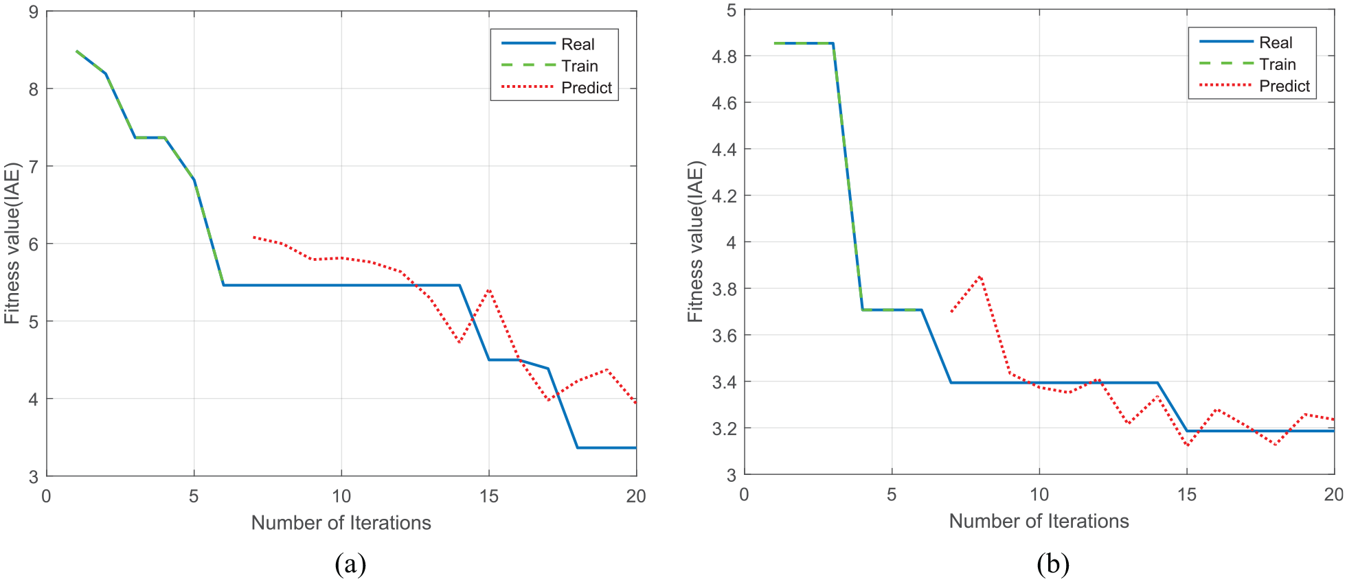
The initial training followed by prediction with real fitness values (IAE of the position error) by LSTM model for Y-axis by (a) PSO and (b) IPSO methods.
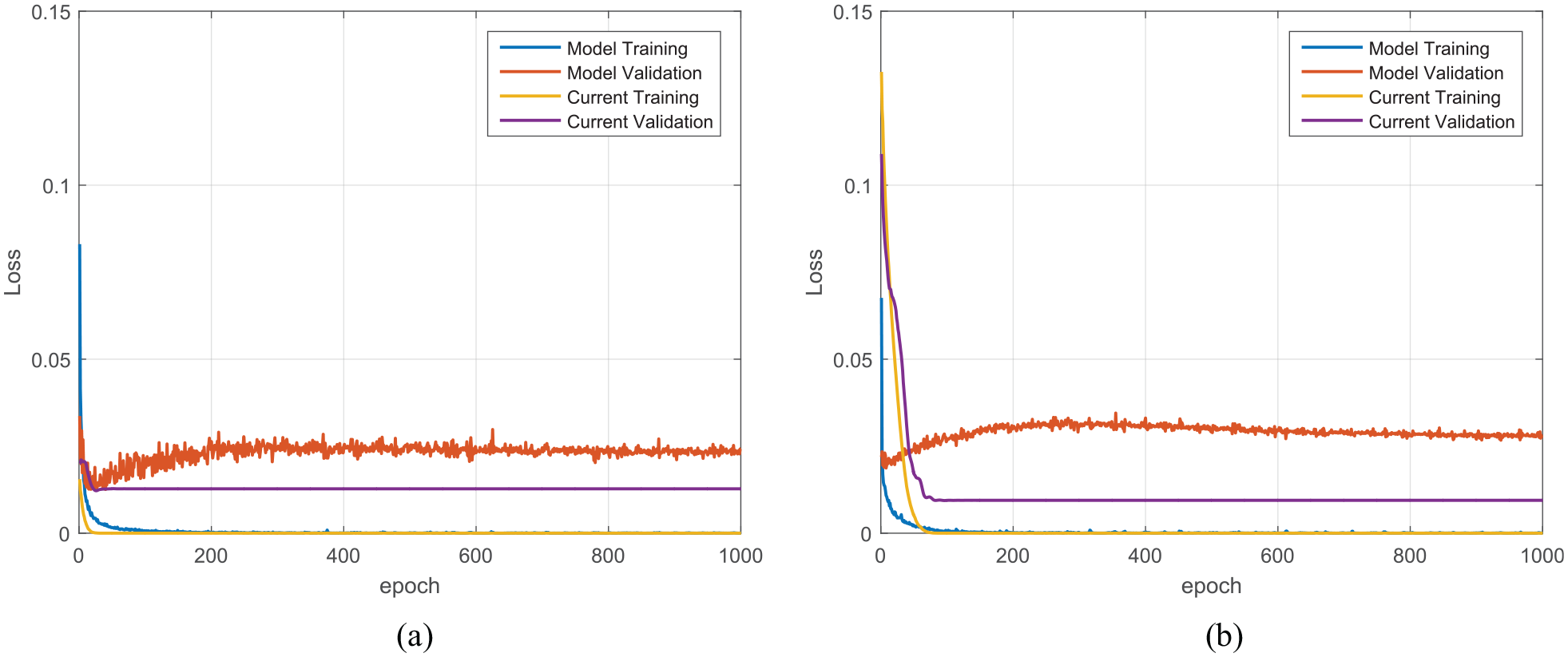
Loss of LSTM model for initial model training (blue), current training (orange), initial model validation (red), and current validation (purple) for Y-axis with PSO (left) and IPSO (right): (a) PSO and (b) IPSO.
X-axis experiments
Next, PSO was used to search for the optimal control parameters for XXY stage motion along the X-axis. The motion command was to move 1 mm at 1 mm/s; the stage’s movement in the X direction was driven by two motors, X1-axis and X2-axis, simultaneously. Therefore, the gantry parameters of the two motors, GKp and GKv, required adjustment for the X-axis. Since, the XXY stage is coplanar, and the structure of the two motors is similar. Neglect all the mechanical error, the Kp, Ki, Kd, and Kff were the same for the two motors. The parameters of the PSO algorithm were as follows: The dimensions were set to 6 (in Table 2), representing the six control parameters, Kp, Ki, Kd, Kff, GKp, and GKv, for the two motors; the range of the parameters was set to 0–10,000; the maximal number of iterations was set to 20; the number of particles was set to 20; the learning factors (c1 and c2) were set to 2; and the inertia weight w was set to 0.6. In the IPSO experiment, maximal inertia weight wmax was set to 1, and the minimal inertia weight wmin was set to 0.2. The experiment was terminated when PSO or IPSO reached the maximal number of iterations.
The control parameters for the X-axis motion of the XXY stage that were obtained through PSO did not reach the target within the error of 1 mm. This may have been caused by mechanism or image error (Figure 18). The fitness values obtained through PSO and IPSO were 6.165 and 5.933, respectively. IPSO was able to search lower fitness. When GKp and GKv were added, the search conditions became more complex. The control parameters identified during the experiment were dissimilar, but the dynamic response of the stage with the PSO and IPSO optimization was still similar, which means that there were many solutions for the optimal control parameters of this experiment. Resulting PSO dynamic response data are as follows: Mp was 7.34%, Ess was 4.6%, and Ts and Tr were 1.11 and 0.84 s, respectively. The IPSO obtained superior fitness values: Mp was 7.33%, Ess was 4.5%, and Ts and Tr were 1.08 and 0.84 s, respectively. Table 3 presents the details.
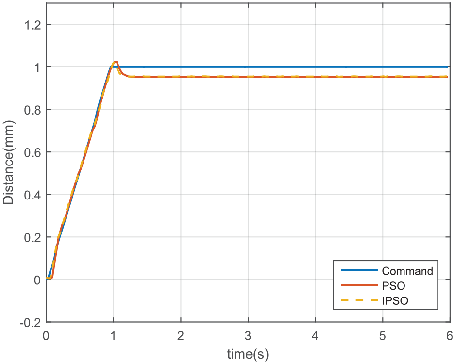
X-axis step response by PSO and IPSO.
Indices of X-axis performance for controller tuned by PSO and IPSO.
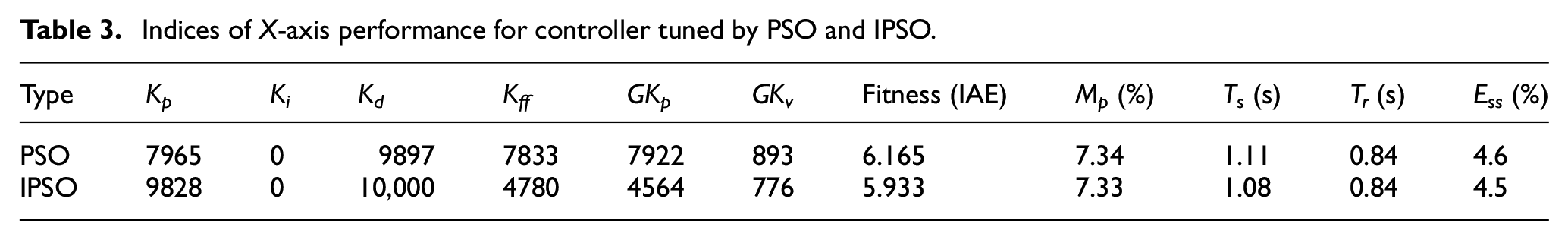
Figure 19 presents the particle parameter distribution diagram for PSO and IPSO. PSO exhibited apparent convergence by the seventh iteration (number of iterative particles = 160), and IPSO exhibited apparent convergence by the fourth iteration (number of iterative particles = 100), which was caused by initial higher w effect. IPSO started with a higher w at the beginning of the iteration and obtained lower fitness and exhibited fewer iterations. Still, the fitness values obtained through these two methods and their step responses were quite similar in Figures 18 and 20.
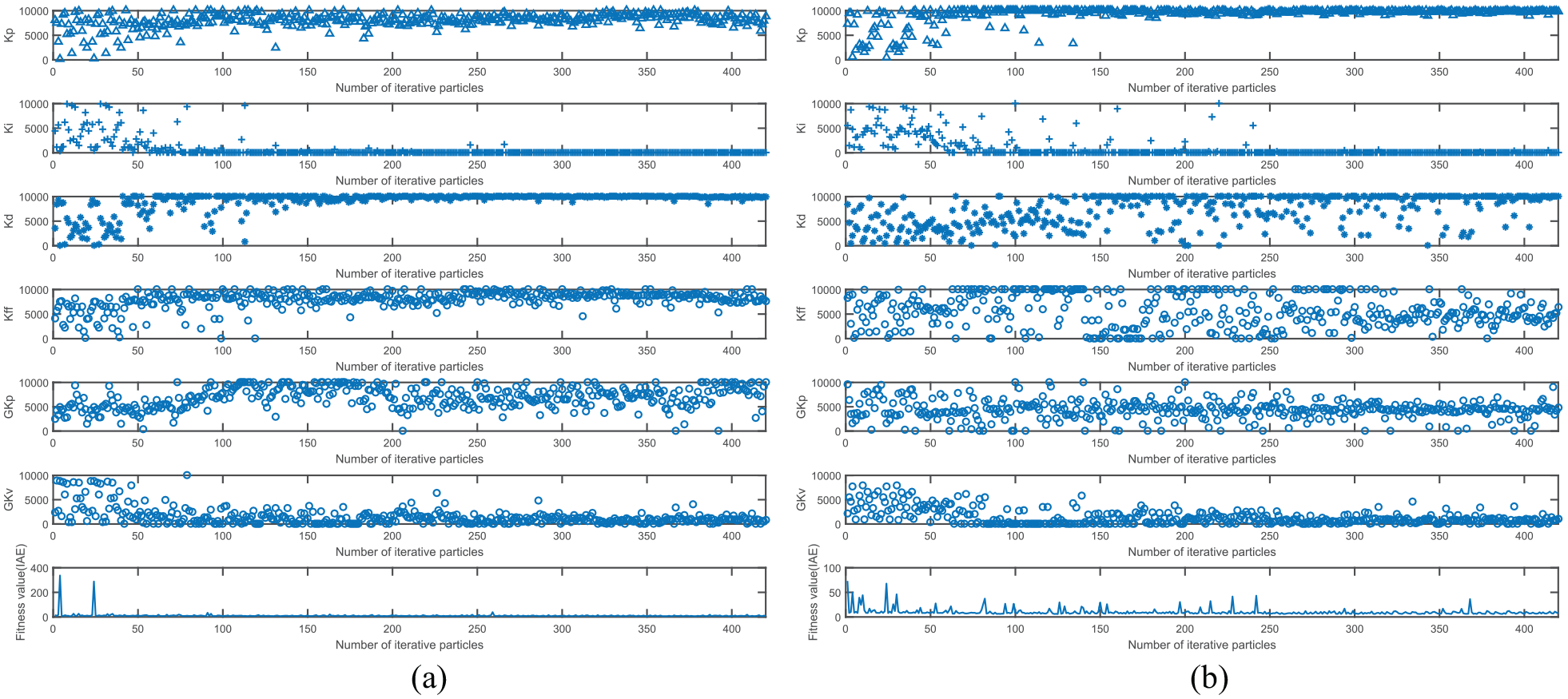
(a) Variation of PID controller gains, feedforward gain, and fitness value with number of iterative IPSO’s particles in X-axis and (b) variation of PID controller gains, feedforward gain, and fitness value with number of iterative IPSO’s particles in X-axis.
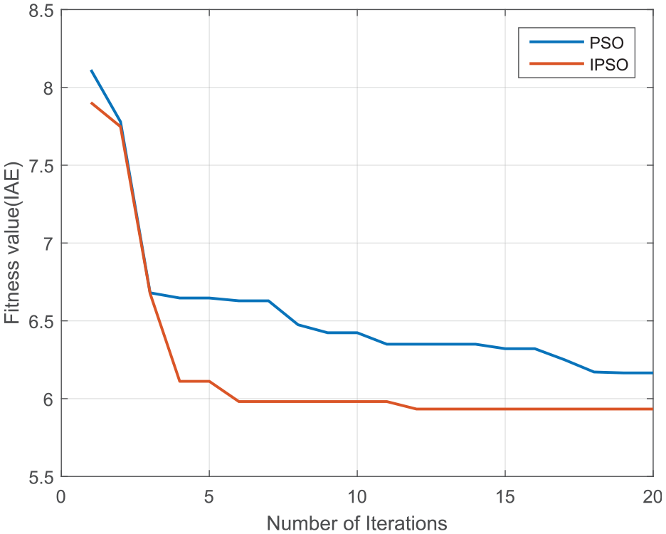
PSO and IPSO fitness value for X-axis.
During the seventh PSO search, the data from the previous PSO search were input to the LSTM model for training, and the parameters of the 20 particles were used to predict the optimal fitness. After LSTM’s model prediction, the curve for predicted fitness was highly similar to the curve in actual fitness value. When the PSO search reached a stable level of fitness value during the sixth and seventh iterations, the prediction curve did not noticeably change. This stable level of fitness was used to determine whether to stop the PSO search (Figure 21). As shown in Figure 22, the loss of LSTM model and current validation by PSO is reduced from 0.05 to 0.005, and the IPSO is reduced from 0.022 to 0.003, while the training loss of PSO and IPSO are both close to 0 (Figure 22). This concludes through the training of the LSTM model, the stage positioning error and time of optimal control parameters in X-axis can reduced significantly with the assistance of LSTM model’s prediction for in-line processes.
The initial training followed by prediction with real fitness values (IAE of the position error) by LSTM model for X-axis by (a) PSO and (b) IPSO methods.
Loss of LSTM model for initial model training (blue), current training (orange), initial model validation (red), and current validation (purple) for X-axis with PSO (left) and IPSO (right): (a) PSO and (b) IPSO.
Circular motion experiments
Next, PSO was used to search for the optimal control parameters for the XXY stage to move a circle by three axes. The radius of the circle was set to 1 mm, the speed was set to 1 mm/s, and the stage’s movement along the X-axis was driven by the two motors, X1-axis and X2-axis, simultaneously. The stage’s movement along the Y-axis was driven by the motor Y-axis. The two gantry control parameters, GKp and GKv, required adjustment for the X-axis movement. Because single-axis control was used for the Y-axis, the gantry parameter for the Y-axis was 0. Because the XXY stage is coplanar, the structure of the motors is similar. Kp, Ki, Kd, and Kff were the same for the three axes. The parameters of the PSO algorithm are as follows: The dimensions were set to 6, representing the six control parameters, Kp, Ki, Kd, Kff, GKp, and GKv, on the three axes. Table 1 presents the parameters. The fitness value for the circular motion was circularity. The results for control of the three-axis circular motion of the XXY stage are presented as circularity data. Once the farthest and closest distances have been calculated, then the circularity value results from a simple subtraction between them. The experiment was terminated when PSO or IPSO reached the maximal number of iterations.
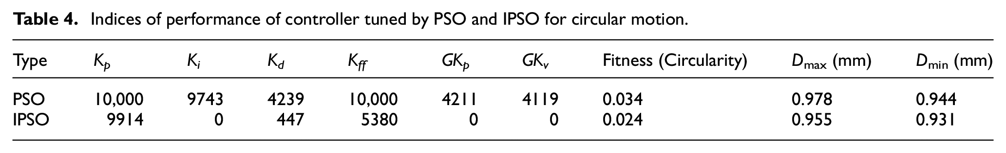
With PSO used to obtain the control parameters for circular motion, the radius of the circle did not reach 1 mm. This may have been caused by mechanism or image error (Figure 23) The fitness values obtained through PSO and IPSO were 0.034 and 0.024, respectively. IPSO identified lower fitness value by using a lower w. For PSO, the farthest distance Dmax was 0.978, and the closest distance Dmin was 0.944. For IPSO, the farthest distance Dmax was 0.955, and the closest distance Dmin was 0.931. The two sets of data were compared. IPSO was able to approximate the circle control parameters. Table 4 presents the data. Figure 24 presents the particle parameter distribution diagram for PSO and IPSO. PSO exhibited clear convergence by the second iteration (number of iterative particles = 60), and IPSO exhibited clear convergence by the fifth iteration (number of iterative particles = 120). Although IPSO did not search the optimal parameters as quickly, its fitness value was superior to that of PSO in each iteration because w decreases at each iteration for convergence (Figure 25).
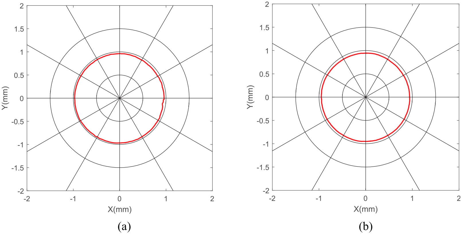
Trajectory of circular motion by PSO and IPSO tuning: (a) PSO and (b) IPSO.
Indices of performance of controller tuned by PSO and IPSO for circular motion.
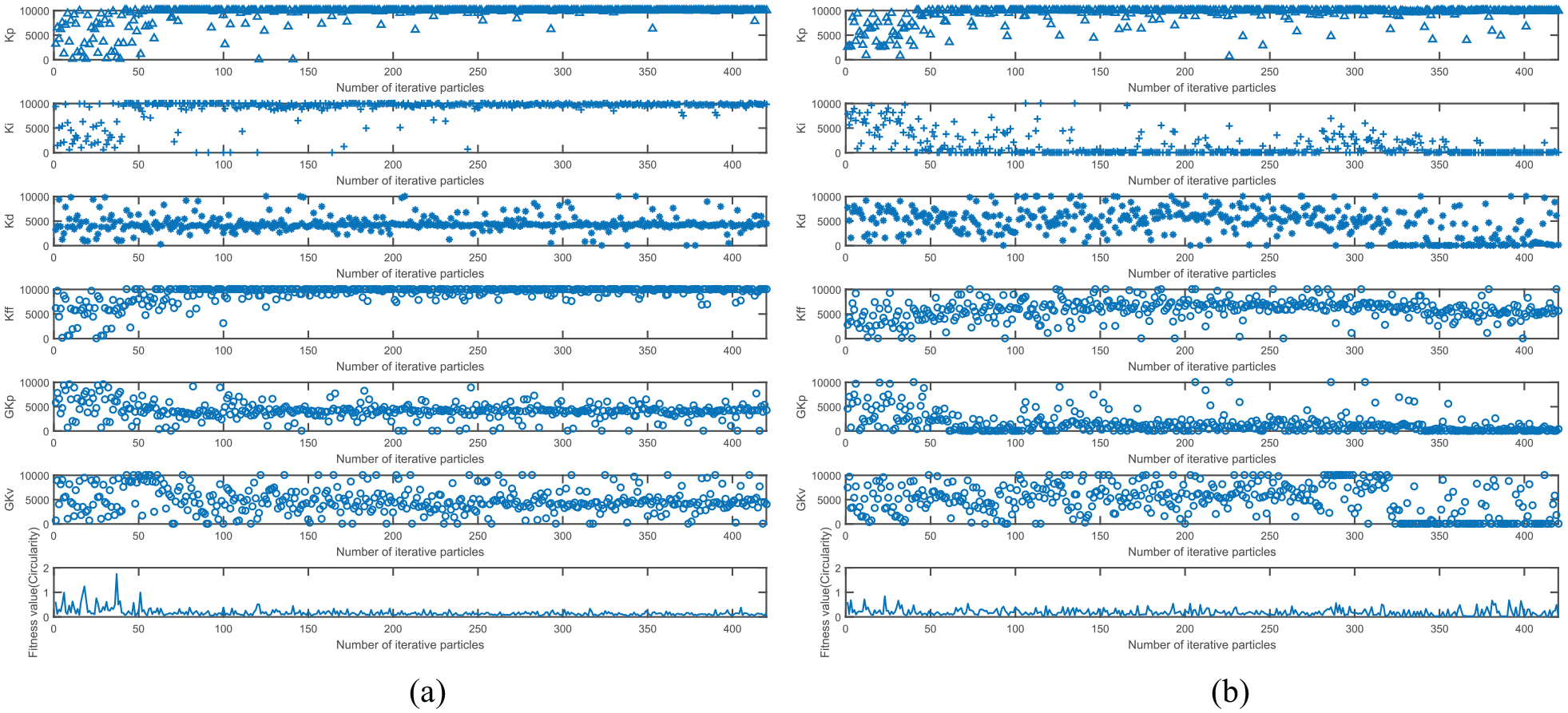
(a) Variation of PID controller gains, feedforward gain and fitness value with number of iterative PSO’s particles in circular motion and (b) variation of PID controller gains, feedforward gain, and fitness value with number of iterative IPSO’s particles in circular motion.
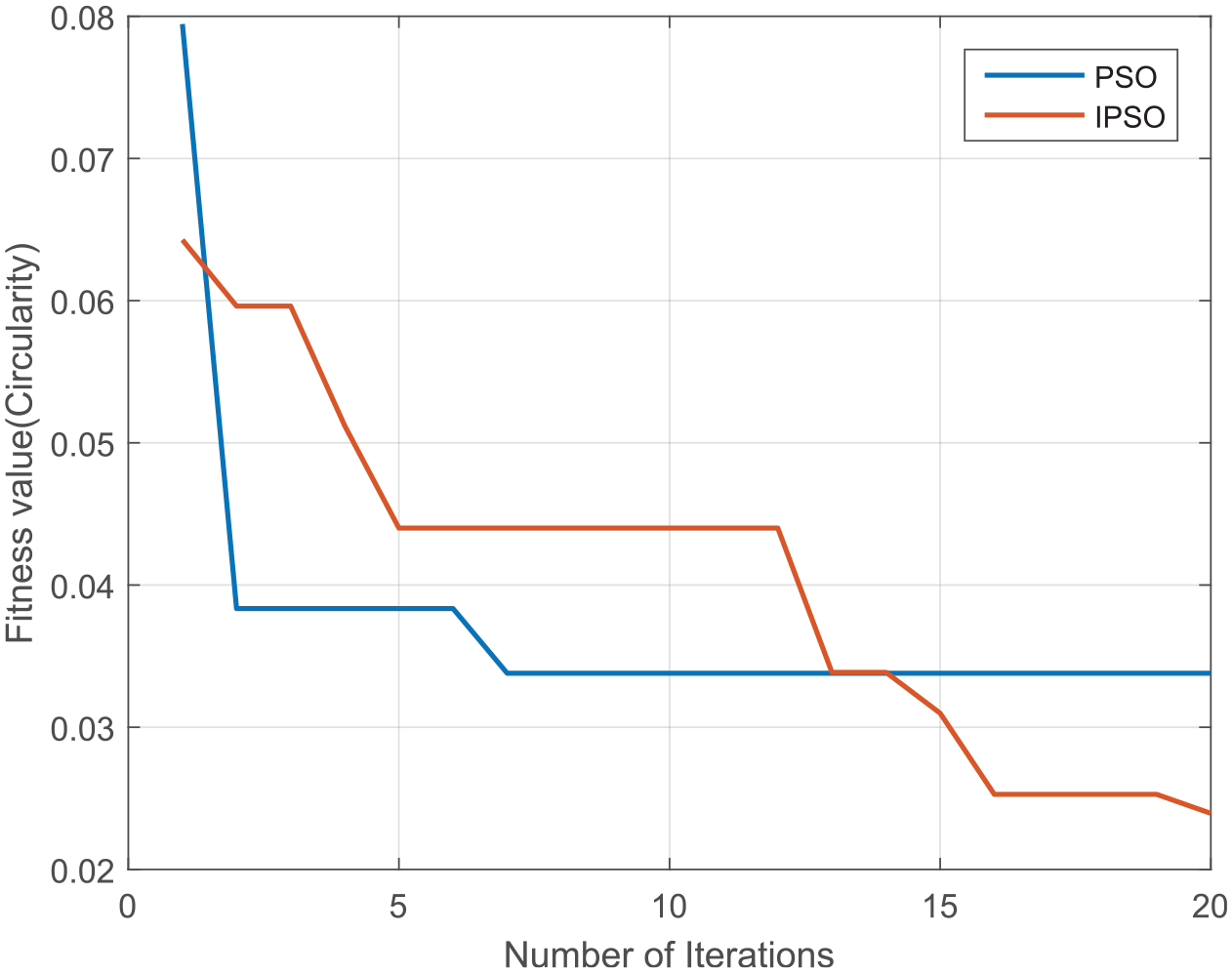
PSO and IPSO fitness value with number of iteration as circular motion.
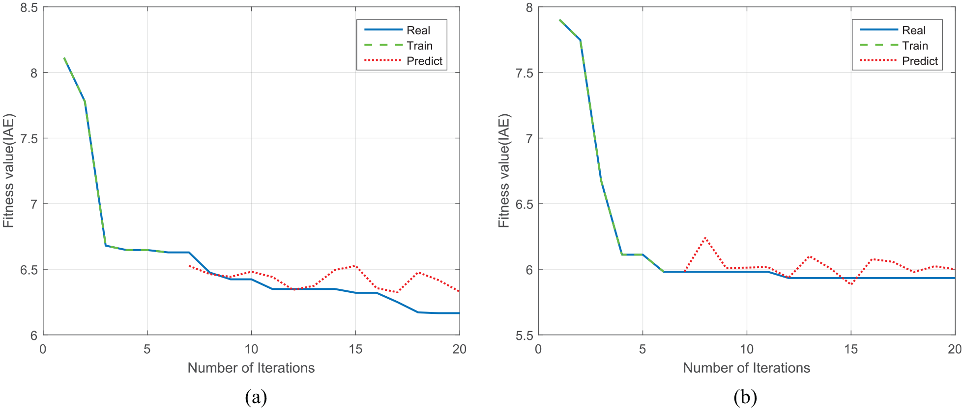
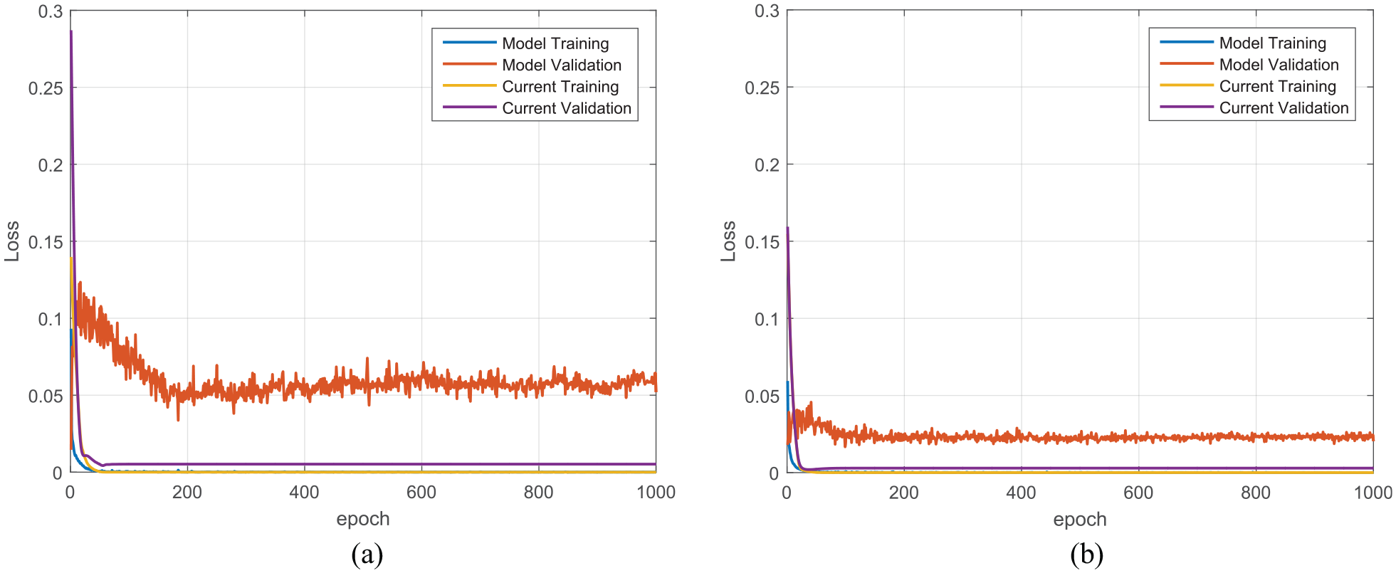
With the same seven PSO searches, the fitness curve LSTM prediction was highly similar to the actual fitness curve. In Figure 26, the LSTM predicted the downward trend for the fitness curves by the PSO and IPSO optimization processes. This allowed whether the PSO or IPSO carries the clear-cut decision to continue searching the best optimal parameters or not. Figure 27 shows the loss of model for current validation via PSO is reduced from 0.004 to 0.002, and the IPSO is reduced from 0.01 to 0.008, the training loss of PSO and IPSO are both close to 0.
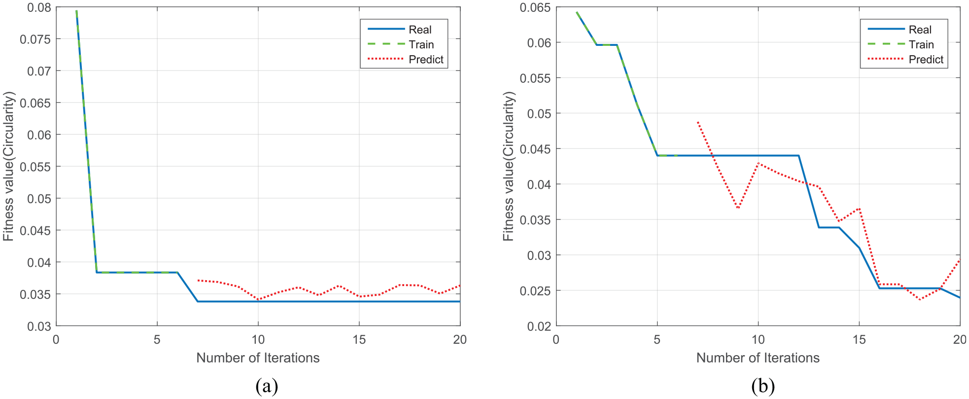
The initial training followed by prediction with real fitness values (IAE of the position error) by LSTM model for circular motion by (a) PSO and (b) IPSO methods.
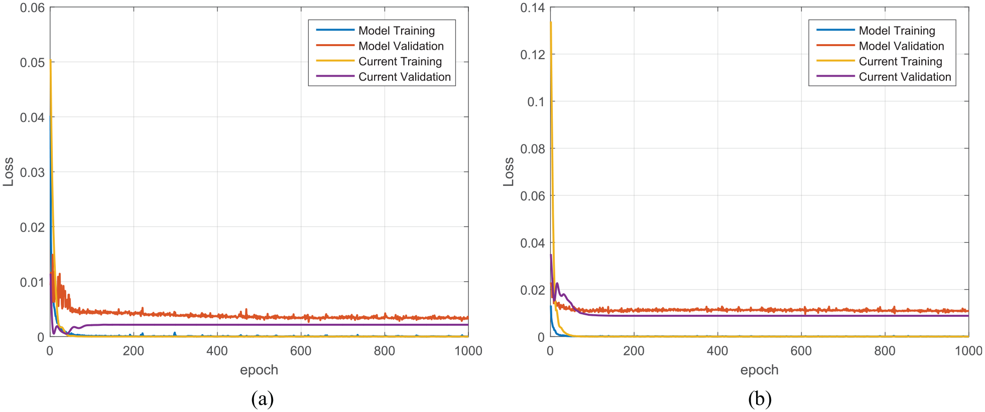
Loss of LSTM model for initial model training (blue), current training (orange), initial model validation (red), and current validation (purple) for circular motion with PSO (left) and IPSO (right).
Conclusion
This paper used PSO and IPSO to obtain the six controller parameters for the precision motion control of the XXY stage. The bettering movement accuracy by the PSO optimization was calculated using image feedback automatic optical inspection system. The dynamic positioning performance was evaluated thereof. PSO control system associated with established long short-term memory (LSTM) prediction models with the functions of learning, storing, and transmitting memory for monitoring the value of fitness function of the controller parameters was implemented successfully. This can reduce the search of control parameters time with a prognostic-diagnosis-like manner for the multi-dimensional parameters demands.
Experimental results showed the PSO-LSTM and IPSO–LSTM based models improved tracking accuracy both for linear and circular trajectories. Therefore, replacing linear optical scales with CCD cameras to capture the stage positioning by PSO-LSTM based controller is feasible. Through the training of the LSTM model based on the PSO’s or IPSO’s information, the fitness function of PSO and IPSO can be predicted effectively. Therefore, the time of optimal control parameters searching in single translation movement (Y-axis), synchronous moving by two motor (two X-axis motor), and circular trajectory motion can predict the effectively with the characteristics of LSTM model’s prediction for real time application. Proposed method can resolve the consuming time for searching the bettering fitness value in optimization. Especially when the assembly of a precision stage demands time for fine tune of the controller parameters. In practice, knowing the machine positioning accuracy is a key priority when the remaining useful life of motion stage could change after long time operation. As for prognostic health maintenance, proposed method with PSO-LSTM model can deploy with precision equipment in shop floor.
Footnotes
Declaration of conflicting interests
The author(s) declared no potential conflicts of interest with respect to the research, authorship, and/or publication of this article.
Funding
The author(s) disclosed receipt of the following financial support for the research, authorship, and/or publication of this article: The authors thanks the Ministry of Science and Technology for financially supporting this research under Grant MOST 109-2221-E-018-001-MY2 in part.