
Abstract
One of the main goals of submarine designers and researchers is to estimate the influence of submarine fluid dynamics for submarine-based optical tracking and pointing systems. In this study, firstly, based on the basic flow governing equation and hierarchical grids, the numerical simulation method of DNS (direct numerical simulation) is adopted to simulate the seawater flow around the submarine at 6° yaw angle and 107 Reynolds number. Secondly, the transformation equations from the earth coordinate system to the optical axis system have been deduced and the ultimate influence of pressure torques on the tracking system is studied. Transfer functions of the coarse channel direct current (DC) torque motor and fine channel fast steering mirror (FSM) also have been modeled and deduced. On this basis, the time domain step responses of both subsystems are analyzed by MATLAB Simulink. Finally, performance analyses have been deduced by comparing the error variation and vortices evolution. It revealed that the frequency characteristics of multi-scale pressure pulsation mainly depended on the lengths of submarine hull or its appendage, as well as the fluid dissipation and random interaction. In general, the coarse channel appears a good compensation performance at low frequency and large amplitude error that caused by the middle-scale pressure pulsation. Contrarily, the FSM fine channel exerts an excellent control effect for higher frequency and small amplitude error caused by small-scale pressure pulsations.
Keywords
Introduction
Different from conventional photoelectric tracking system, laser directed energy device needs to guide and keep the laser beam continuously and stably focused on the target. 1 The tracking accuracy must be one or two orders of magnitude higher than the conventional weapon. Originally, only equipped with periscope, submarine-based photoelectric mast has become an advanced image acquisition and automatic tracking device controlled with computer in recent years. 2 In further, laser directed energy device is a promising application on submarines with the continue miniaturization of high energy laser equipment. Therefore, it is necessary to deeply study the mechanism of vortex induced vibration for the disturbance error of submarine-based laser directed energy device.
When submarine moves at high speed underwater, the boundary-layer separation and flow field perturbation around the submarine and its appendages will be generally formed. In the case of high Reynolds number, tip vortexes will be generated at the end edge of the hull or appendages of the submarine accompanied by large force and torque fluctuations. In hydrodynamics, large low pressure area will be formed in vortex cores, and cavitation pittings will be aroused once the pressure drops to a certain degree. 3 Not only will strong pulsations produce extremely unfavorable vibration and noise, but it also reduces the stability or concealment of the military submarine.
Besides tip vortices, turbulence vortices characterized by different multi-scales and shapes are induced from the submarine body and its appendages. Depending on their scales, the evolution of turbulence could mainly be divided into three stages. The first is the slowly decay period of large-scale vortices, during which stage the large-scale vortices decay slowly and mainly affected by the fluid’s convection and diffusion interactions rather than the dissipation. The second is the fast decay stage of medium scale vortices, during which period the large-scale vortices cannot keep their former shapes and then fast broken with the existing time being the least for the whole period. The third is the small-scale vortices dissipation stage; the fluid’s convection tends to weak and the convection time is the longest.
The turbulent vortex always changes randomly and rapidly over time and space. The interactions of turbulent and hull will lead the problematic noises. On the one hand, the random pressure pulsation directly produces radiated noise; on the other hand, the elastic structure of hull’s surface material will vibrate and produce radiated noise, which is collectively classify as “hydrodynamic noise”. 4 Unfortunately, the vibration or noise inevitably restricts the tracking precision of the laser directed energy device. 5
At present, a great deal of investigations have been carried out on submarines under different navigational conditions. However, numerous investigations have been widely conducted focused on submarines, under various navigation conditions. Predictive capabilities of hybrid RANS/LES models were compared for single-phase flow over a surface combatant at Re = 5.3 × 10⁶ and an appended the DARPA SUBOFF model at Re = 1.2 × 10⁷. 6 Alin et al. 7 discussed some features of submarine hydrodynamics, engaging in further studies on the DARPA SUBOFF configurations a bare hull and a fully appended model. Based on the differ DARPA Suboff models, Xing et al. 8 identified and analyzed the vortical and turbulent structures, instabilities, with analogy to the vortex breakdown and helical instability analysis for delta wing at large angles of attack.
The hydrodynamic characteristics of the same model are similar to the disturbance mechanism, so we only analyzed the condition of Re = 107 and attitude at 6° yaw angle. In the third section of this paper, based on the basic control equations of fluid mechanics and the hierarchy grids, seawater flow around the submarine has been numerical simulated. In section 4, coordinate transformation methods have been deduced. In section 5, based on the multi-scale visual vortices, the torque disturbance in optical axis coordinate system has been investigated. The sixth section deduces the mathematical models of torque motor and FSM, according to the design mechanisms of torque motor and permanent magnet synchronous motor. And then by MATLAB Simulink toolbox, the effect of submarine disturbance on the coarse/fine channels output errors are simulated and analyzed. In section 7, according to the vortex field evolution characters, the influence factors and internal mechanism between the pressure pulsation and tracking precision of submarine-based optical system have been further revealed.
System descriptions
Except for algorithm filtering, adaptive optical frameworks are generally adopted to compensate the disturbance angle error in order to enhance the anti-disturbance capability as well as the stable tracking capability of tracking and aiming servo system. Recently, FSM, as an important optical path adjusting device, has been widely used for precise adjustment and stabilization control of optical axis, 9 which is primarily composed of piezoelectric ceramic stacks, a closed loop controller and a loaded mirror. Compared with the torque motors in coarse channel, the FSM in fine channel offer several advantages such as higher angle control precision (the repeatable positioning accuracy is about 5–20 urad) and high operation bandwidth (about 0.2–1 kHz), which will be discussed in the following paper.
Figure 1(a) shows the laboratory servo equipment we used, which is composed of coarse and fine two channels. The servo equipment is primarily composed of two coarse channel azimuth/pitch rotary platforms, two torque motors, a FSM, a charged coupled device (CCD) and a wedge-shaped body with 45° inclined plane. During the experiment, the laser is generated from a small laser source loaded on the right platform in front of the FSM. Laser beam is reflected by FSM, and then passes through the round hole. Finally, through 45° wedge mirror the laser is adjusted and shot toward the target. Two DC torque motors are selected to drive the altitude and the azimuth platforms, avoiding the gear clearance error.
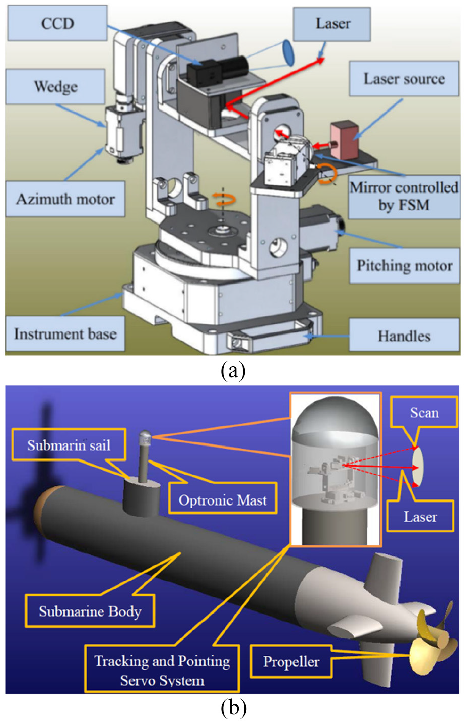
Diagram of submarine tracking and aiming equipment: (a) structure of tracking and aiming system and (b) conception of tracking and aiming servo system on the submarine.
In practical, servo equipment in Figure 1(a) will be loaded at the optical mast in Figure 2(b). Firstly, the target is detected by radars or photoelectric detection devices to guide the submarine-based tracking and aiming equipment and catch the target. Secondly, when the coarse channel intends to track stably, the fine channel FSM will be enabled and guide the laser shot on the target more precisely, as shown in Figure 1(b).
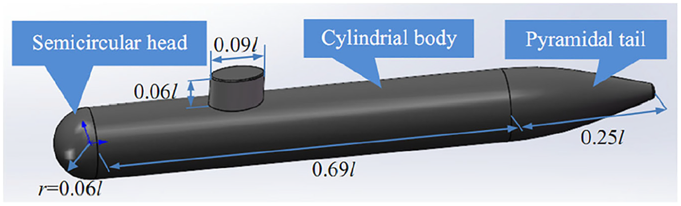
Submarine model in numerical simulation.
Basic model and numerical method
Basic model
Figure 2 shows the submarine model’s scales, which is composed of a semicircular head, cylindrical body and pyramidal tail, with corresponding lengths of 0.06l, 0.69l, and 0.25l, respectively, where l is the submarine length and also the characteristic length in this simulation.
Total size of computational domain is 4l × 2l × 2l, free stream flow along the X-axis positive direction, the leading edge point of the submarine located at the origin of right-handed coordinate system and keeping 0.5l away from the inlet surface. The X-axis points to the downstream, the Y-axis points to the starboard, and the Z-axis points to the vertically upwards. In this simulation, for the computational domain, the left and right surfaces are defined as speed entry and pressure outlet boundary conditions with constant pressure and velocity in normal direction being zero. Additional, the submarine surface is defined as no-slip boundary condition.
Numerical method
Governing equations
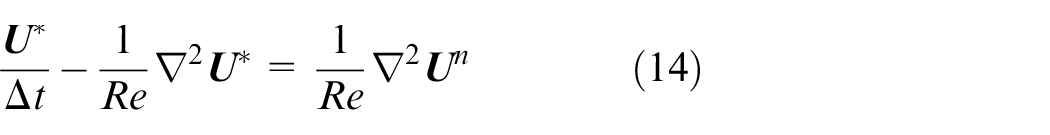
In the computational domain the dimensionless viscous incompressible flow governing equations can be written as:

Spatial discretization
The computer domain is spatially discretized using square (cubic in 3D) finite volumes organized hierarchically as a quad-tree (octree in 3D).10,11 This type of discretization in Gerris software has been applied to solve the governing equations for incompressible flows. 12 Detail descriptions to spatial discretization and the corresponding tree representation are given in Figure 3 and a prior paper. 13
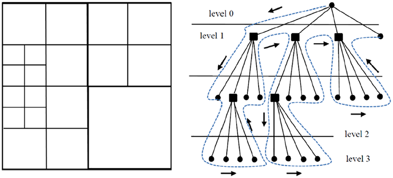
Diagram of quad-tree discrete and corresponding tree structure.
Using the tree structure grid, for the
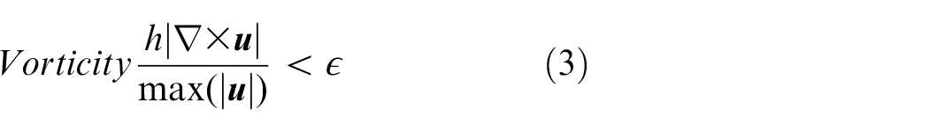
This criterion will ensure that a finer resolution is used in solution areas with higher vorticity values. h the mesh size and
Temporal discretization
The classical projection method is commonly referred to solve these government equations. Base on this Helmholtz-Hodge decomposition that a twice continuously differentiable bounded vector field can be decomposed into a curl-free component as well as another divergence-free component.
13
This projection method relies on Hodge decomposition of the intermediate velocity field

The

By solving the Poisson equation the Hodge variable

The discrete form of the projection operator depends on the discrete position of the corresponding pressure and velocity fields. The convective pressure was projected accurately at the center of the cell surface, while the velocity was selected approximately at the center of the cell.
Therefore, based on the above solution method, at time step n, the control equation can be discretized as:
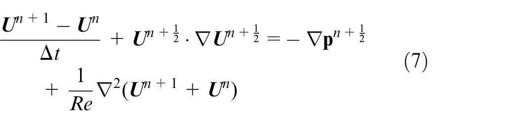


Poisson equation can be written based on the equations (10) and (11).

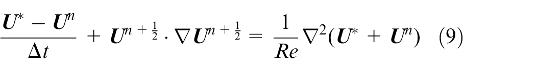
Poisson equation is solved by an Octree-based multistage solver. Discrete momentum equation (9) can be rewritten as:
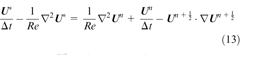
The convection term is discretized by second-order upwind scheme of Bell-Colella-Glaz. The diffusive term is discretized by Crank-Nicholson method, which has second order accuracy and unconditional stability. Above all, in this simulation, both time and space dispersions are of the second order accuracy. 16 Direct numerical simulation, or DNS, a full numerical simulation of a turbulent flow is adopted, which does not rely on any numerical calculation models of the flow.
Grid independence test and experimental verification
In order to verify that the grid layer number has no effect on the results as well as the correctness of the numerical simulation method, the calculation grids and results for four different kinds of grid layer numbers (Nlevel = 6, Nlevel = 7, Nlevel = 8, and Nlevel = 9) have been numerical investigated based on the SUBOFF bare model are shown in Figure 4. 17
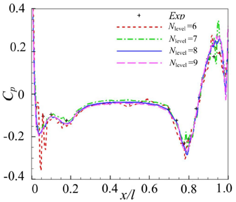
Pressure coefficient distributions of the submarine middle section under different grid layers (Exp. is experimental result). 18
Figure 4 shows that pressure coefficient Cp distributions on the section of the hull with four different grid layers. As shown, these Cp distributions have relatively consistent and closely change trend with the experimental results. And with the increasing of grid layers, the calculated pressure coefficients tend to more precise consistent with the experimental result 18 . In addition, based on this flow field calculation method, the flow around a cylinder has be calculated and compared with previous research results at Re = 100, which are available in our former papers.19,20
In order to detect the fluid dynamics microscopic characteristic of the submarine more sensitive, a balance between the computer condition and the calculation complexity should be struck. Therefore, nine layer grids are adopted in this study. In this numerical simulation, the smallest length of grid is
Perturbation solution of the azimuth/pitch angles
It could be assumed that, for very short CCD sampling period
Deduction of translation movements
Figure 5 is diagram of translational motion decoupled. The influences of this motion along X-axis, Y-axis and Z-axis on the azimuth and pitch angles can be described as equations (15) to (17):
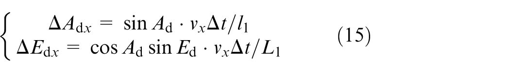
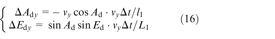

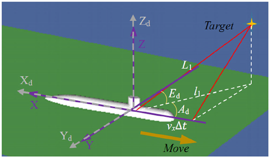
Diagram of translational motion decoupled.
Through ignoring the coupling interaction from three different translational disturbances, the azimuth and pitch angles can be written as:
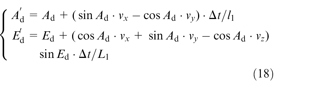
In tracking and aiming systems, the necessary frame frequency for image processing
Deduction of swing movements
The azimuthal angle and pitch angle of target G (x, y, z) in submarine coordinate
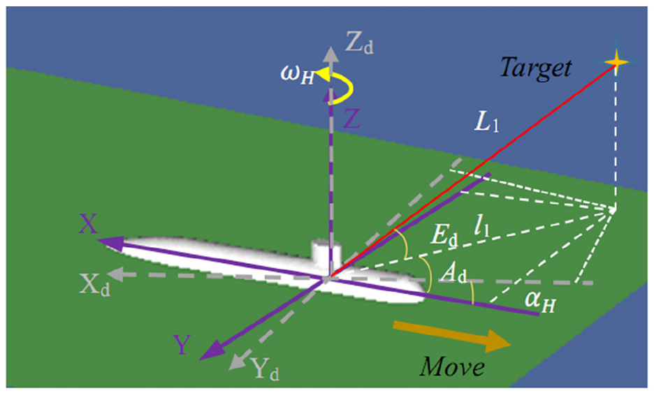
Diagram of rotational movement decoupled (yaw).
Three steps needed when convert the coordinates of the target point in the earth coordinate system
Three transitions could be solved in the matrix form as following equations (19) to (21):
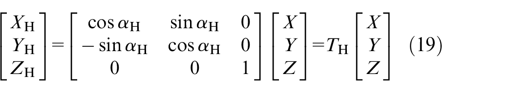
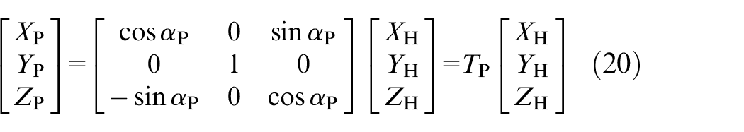
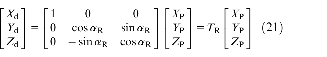
Combine the above three equations it could be obtain:
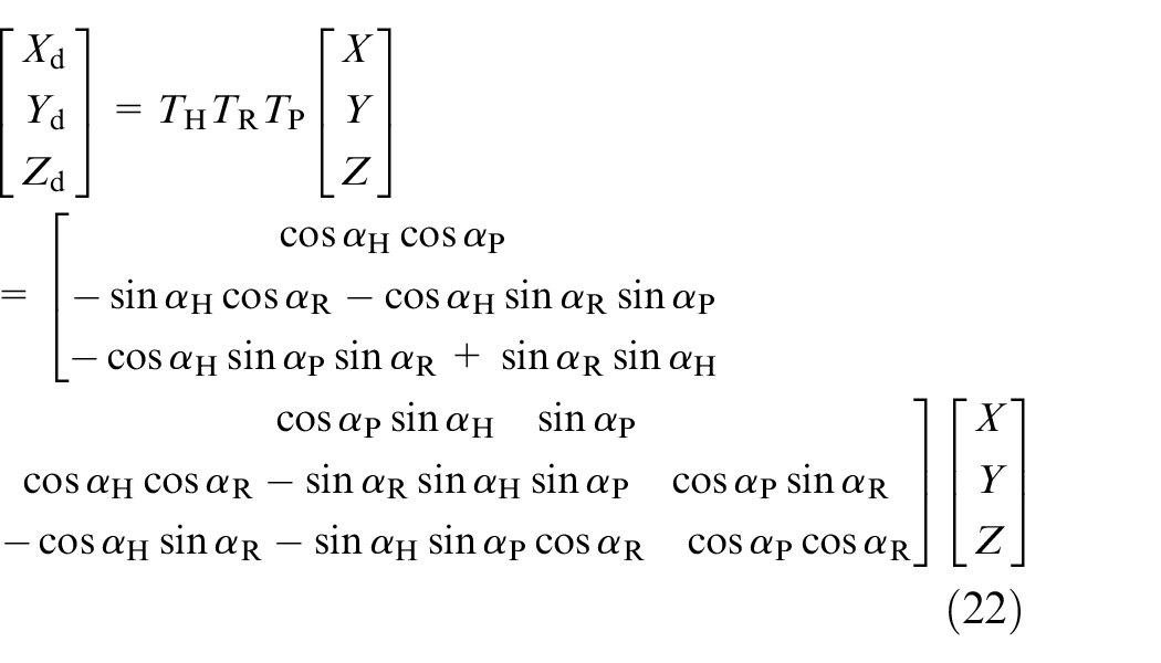
The coordinate points
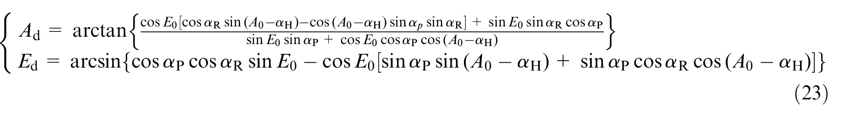
Where the
Submarine torque and flow field characteristics
In this paper, the evolution of torque coefficients are discussed and used to reflect the disturbance characteristics of submarines. The total pressure difference torque coefficient and viscosity torque coefficient in three directions are defined as
Figure 7 displays that the
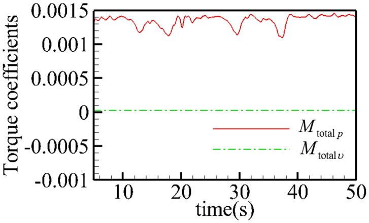
Time histories of the total pressure
Eventually, the torque’s influence on the photoelectric mast and tracking device will be reflected in azimuthal and pitch angles, whose strength are mainly related with the submarine mass and the reference coordinate system. The transformation between the torque and disturbance angles can be regarded as a linear relationship. In numerical analysis, we define
Once considered as an unrestraint rigid body, submarine could move and roll freely with six degrees of freedom (translational motion three, rotational motion three). However, in this simulation, we suppose that pressure does not change the submarine attitude. Usually, pressure pulsation is defined as the pressure fluctuate around its mean value
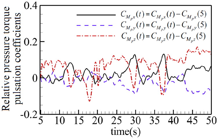
The pressure torque pulsation coefficient curves from 5 s.
In this discussion, these rotation tendencies or the angles around the earth coordinate system are totally caused by the fluid dynamic moment’s waves. However, during the whole simulation process, the submarine keeps a same attitude. Combined with the momentum theorem, the moments can reflect an object’s rotation motion around its rotation center. Thus, the waves of
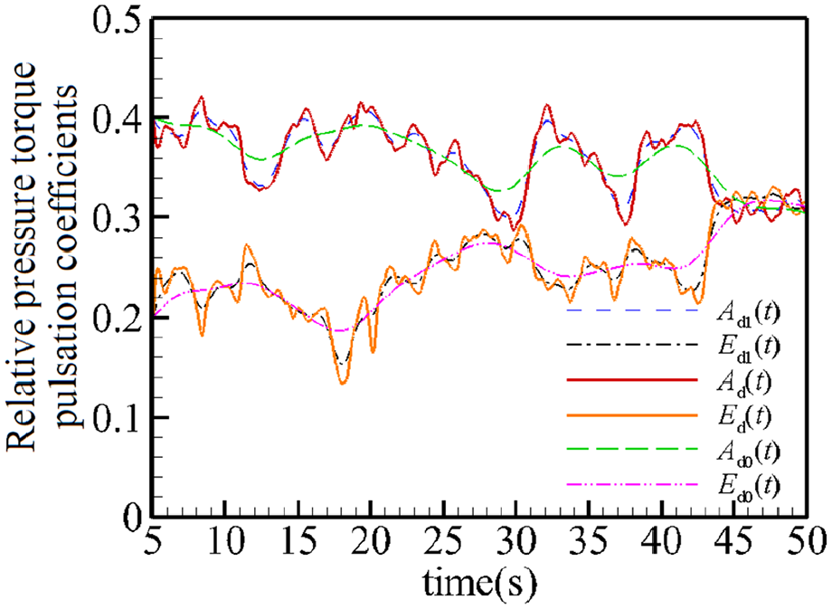
Time histories of (Ad(t), Ed(t)), (Ad0(t), Ed0(t)), (Ad1(t), Ed1(t)).
To obtain much more deeply investigate on the effects of different amplitude pressure torque pulsation introduced by different scale vortices, the average filter methods with two differ parameters have been used to convert the (Ad(t), Ed(t)) curves shown in Figure 9 into two different disturbance curves (Ad0(t), Ed0(t)) and (Ad1(t), Ed1(t)). From the perspective of turbulence analysis, mean-filtering is to make the small scale random fluid movement causing the pressure pulsation dissipate and mix together with the surrounded larger scale vortices. Figure 9 is the curves of (Ad(t), Ed(t)) without mean-filtering. (Ad1(t), Ed1(t)) have been processed by high frequency filter, and (Ad0(t), Ed0(t)) are with low-pass filter. As illustrated in Figure 9 the fluctuation amplitudes of (Ad0(t), Ed0(t)) are approximately equal to 0.1, with their periods being about 0–15 s. (Ad1(t), Ed1(t)) wave around the curves of (Ad0(t), Ed0(t)) and it also contains small period’s oscillations about 2–3 s. The original curves (Ad(t), Ed(t)) contain both the fluctuation characteristics of (Ad1(t), Ed1(t)) and also characterized by the random pulsation traces at small amplitude and higher frequency.
Mathematical connotation of vortex strength is the mean variance of the flow field velocities curl in three directions, which reflects the rotation trend of space fluid. The interaction between the rotational fluid and the submarine surface viscosity boundary causes the pulsation of pressure torques. In order to get a deeper investigate on the time histories of pressure torque pulsation coefficients shown in Figure 9. Vortices evolution characteristics from t = 30–41 s have been listed in Figure 10.
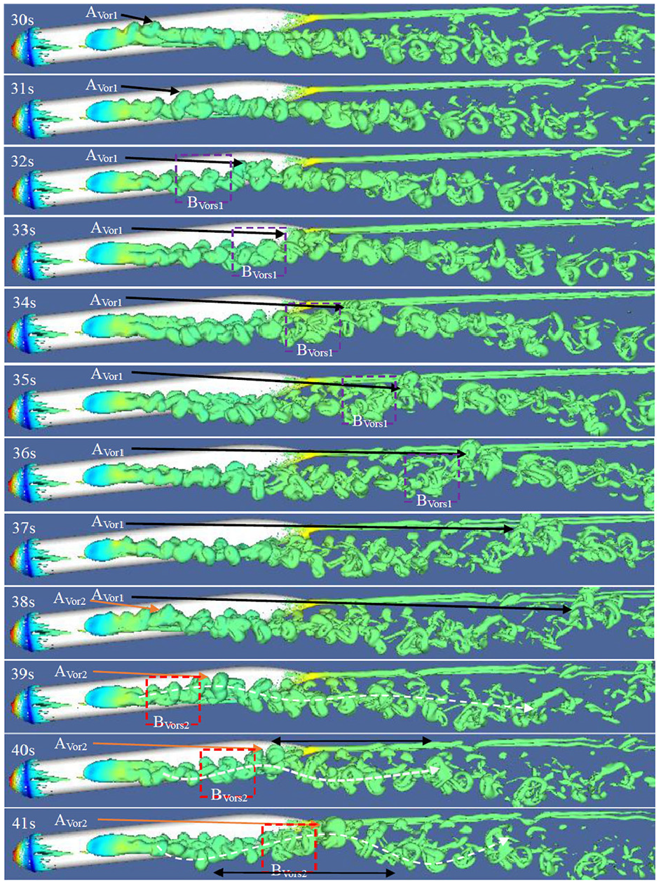
Vortices’ evolution characteristics from t = 30–41 s.
Figure 10 displayed the whole development process of vortex structures from 30 s to 41 s. The structures are visualized as iso-surfaces of vorticity, where the color indicates the local pressure. It can be seen that a large-scale A-kind vortex denotes as Avor1 begin to shed from the upside of the conning tower. The Avor1 vortex could keep the original shape and move toward downstream during the following 3 s 31–33 s. Since 33 s, Avor1 moves out of the submarine body and dissipated into several medium-scale vortices. With time going on, the medium-scale vortices developed from the Avor1 vortex are gradually transformed into a variety of small scale vortices and spread into the surrounding flow field.
By comparing the flow field at 32 s and 31 s in Figure 10, multiple small Bvors1 sub-vortices appear in the purple dotted line frame within 1 s. These Bvors1 sub-vortices are followed the Avor1 vortex closely and move to the downstream. The kind of Bvors1 sub-vortices contain lower energy, so that most of them dissipate rapidly and develop into several interlaced smaller-scale vortices when they move out of the submarine. From the perspectives of time, the series of small-scale Bvors1 sub-vortices produce about 2–3 Hz waves, which have reflected on the changes of pressure torque pulsation coefficient, as shown in Figure 9. Comparing the filtered Ad1(t) and Ed1(t) with the unfiltered curves Ad(t) and Ed(t), it is detected that the unfiltered curves contain more small amplitude waves at frequcecies about 2–3 Hz, which are aroused from the Bvors1 sub-vortices.
Moreover, the generation mechanism for the B and A-kinds vortices is different. A-kind vortices are generated from the upside of the conning tower, they are of much kinetic energy, lower-frequency and larger-amplitude. Avor1 is followed by Bvors1, showing in the red dotted-line box from 32 s to 36 s. Similarly, Avor2 appears at 38 s about 7 s later than Avor1, which will then continue and repeat the same evolutionary process. A-kind vortices are deducted at the time of 9 s, 17 s, 30 s and 38 s, for the whole process, the corresponding fluctuation peaks and dips also can be detected one after the other from Ad0(t) and Ed0(t) curves in Figure 9.
Furthermore, it could be found from 39 s to 41 s, under the flow’s action, the wake vortex track swing at a large amplitude and longer period. That caused by the submarine hull body whose length is much longer than another appendage. Its fluctuation periods are about 10–20 s ranged from 5–17 s, 17–35 s, and 35–48 s that are reflected by the heaving billows of Ad0(t) and Ed0(t) curves in Figure 9. Compared Ad1(t) and Ed1(t), it is detected that the unfiltered curves Ad(t) and Ed(t) contain much more small amplitude waves, about 2–3 Hz, which are bring about by the Bvors1 sub-vortices.
In general, based on the frequency characters, the azimuth and pitch angle curves Ad0(t) and Ed0(t) can be divided into three forms: the high frequency random small perturbations accompany with B kind vortices about 2–3 Hz, the middle frequency perturbations accompany with A kind vortices about 1/4–1/6 Hz, and the low frequency perturbations about 1/15–1/20 Hz. According to the flow field analysis, the fluctuation of middle/low frequencies are mainly resulted from two parts of submarine that is the hull and appendage. High frequency random small perturbations are generated from vortices motion, which cause fluid’s small pulsation, fluid mix or energy exchange among different fluid layers.
Mathematical model of servo system
Structure and transfer function of the DC torque motor
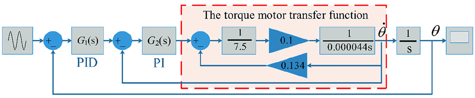
The coarse channel is mainly composed of DC torque motor (DTM) and rotational platform as Figure 11 showing. In this paper, the math model of DC torque motor is deduced.
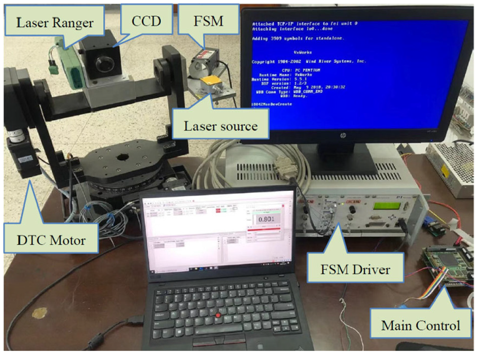
Experimental equipment of tracking and aiming system.
In order to simplify the research, it can be assumed that the electrical parameters and transfer functions of the azimuth torque motor and its rotational inertia are strictly consistent with the electrical parameters and transfer function of the pitch torque motor. Current fluctuation can be ignored and the DC torque motor can be estimated to be a linear device. Thus, based on the principle of motor the voltage balance equation of armature circuit can be obtained:
Where

Where J is the load equivalent torque of inertia,
For this model, the peak torque voltage is 27V, the maximum rotational velocity
In order to improve the response speed, the speed loop adopts PI controller and the position loop adopts PID controller, as shown in Figure 12. For the system, this steady-state error under a unit step response without distribution is about 4.15×10⁻⁵.
Angle error transfer function of the coarse channel.
Structure parameters and transfer function of fine channel FSM
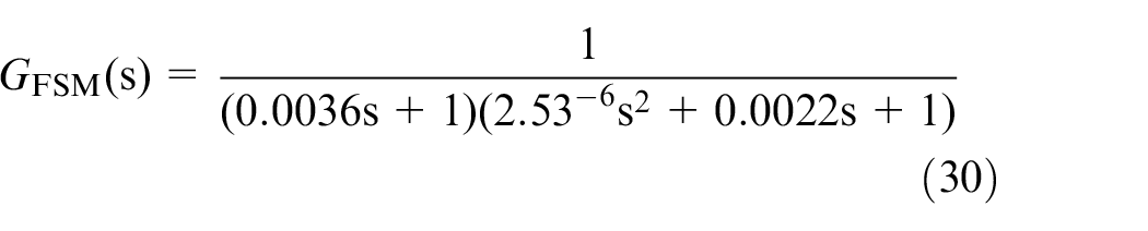
The physical swing magnitude for each axis of the FSM in fine channel is ±12.5 mrad and the closed loop repeat positioning accuracy is 5 μrad. The FSM’s structure is shown in Figures 1 and 11, which primarily composed of a cuboid body, with four moveable coplanar fulcrum points on its head, onto which the mirror is fixed. Through the FSM controller, the length of inside piezoelectric ceramic stacks could be adjusted with the control voltages. Meanwhile, the deflection and pitch angles of the mirror fixed onto the four moveable fulcrum points can be accurately controlled. A spectrum analyzer is used to measure the frequency response curve of FSM in the closed-loop state, and the closed-loop transfer function could be deduced as22,23:
For the fine channel FSM, PID control method is used, its steady-state error under a unit step response without distribution is about 8.1 × 10⁻¹⁵. This control precise can only be reached in theory and idea conditions.
Transfer function of compound axis tracking system
Figure 13 is the MATLAB Simulink simulation diagram of the transfer function for this compound axis tracking system. The output of coarse tracking angle errors are then sent to the fine tracking PID controller as its input signal. The fine channel PID controller has the
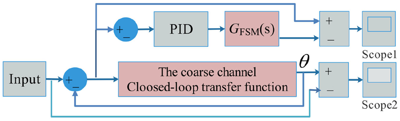
Transfer function of the coarse and fine composite axis.
In order to analyze the system’s robustness, in this numerical simulation, the unit step input signal composed with a continual random disturbance is investigated. For this tracking and aiming system, the input signal contains continuous random input errors of roughly 5% total amplitude and 1 kHz wave frequency. Then the input signal is send to the whole system demonstrated on Figure 13 in MATLAB and Figure 14 is the output response curves obtained from the scope 1 and 2 on Figure 13. The corresponding rise edge of the coarse channel is about 0.15 s. Due to the limitation of the system bandwidth, there is not effective error compensation result was found for the 1 kHz system random disturbance input. Thus, the continual random disturbance has no obvious influence on the stability of the system.
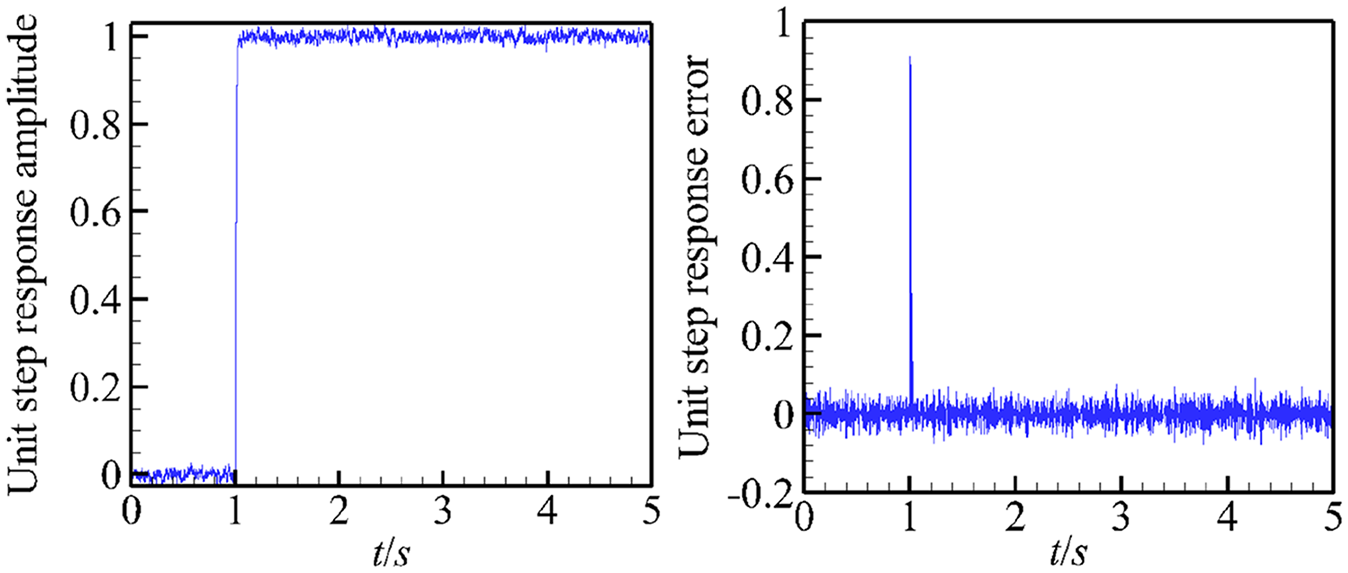
Unit step response added a random disturbance input: (a) coarse tracking output, Scope1 and (b) fine tracking error, Scope2.
Influence of flow field disturbance on steady error
The time histories of
Figure 15(a) to (c) show the tracking error tracks of azimuth and pitch angles through the coarse tracking, which display that under three scale’s disturbances the output errors of azimuth angle
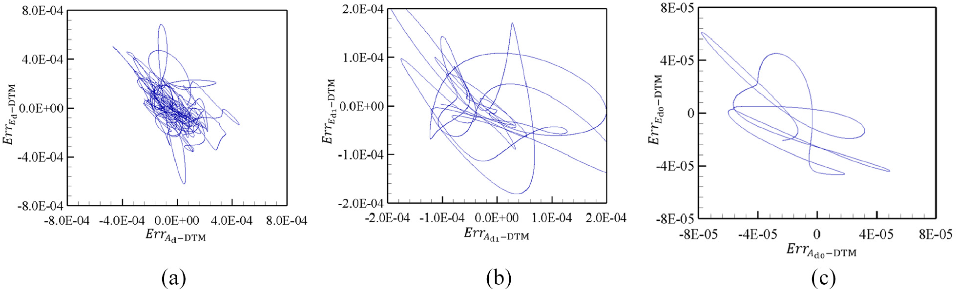
Three track distributions for the coarse tracking errors (a) Without mean-filter; (b) With high frequency filter; (c) With low-pass filter
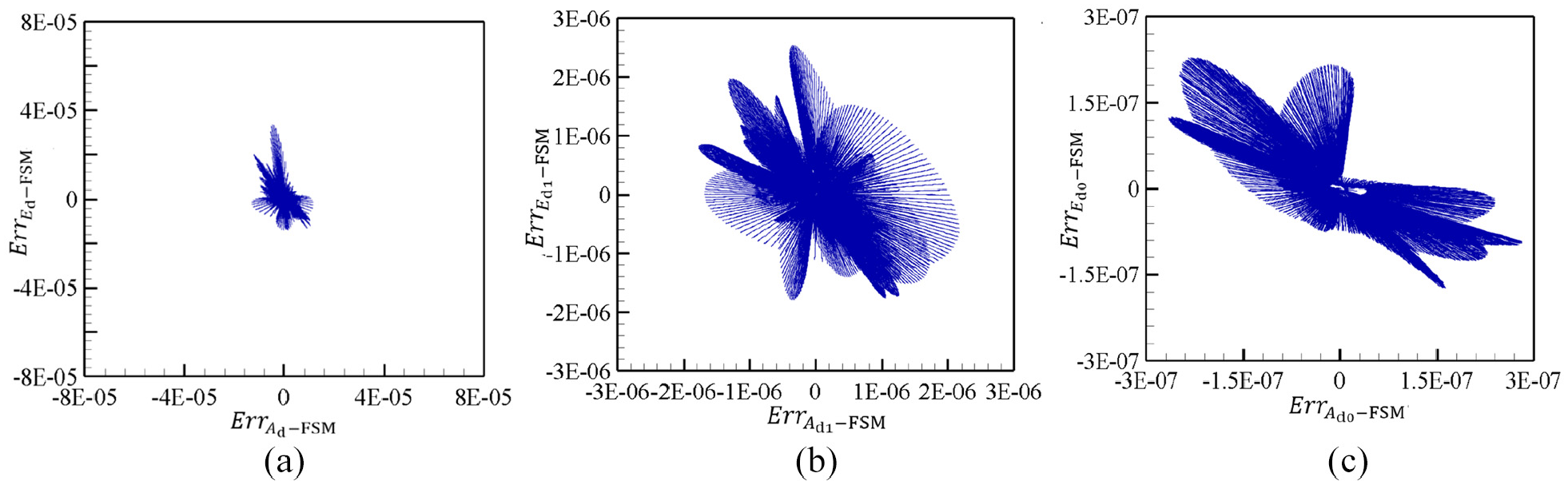
Three track distributions for the fine tracking errors (a) Without mean-filter; (b) With high frequency filter; (c) With low-pass filter.
Error distributions of coarse and FSM/fine channel.
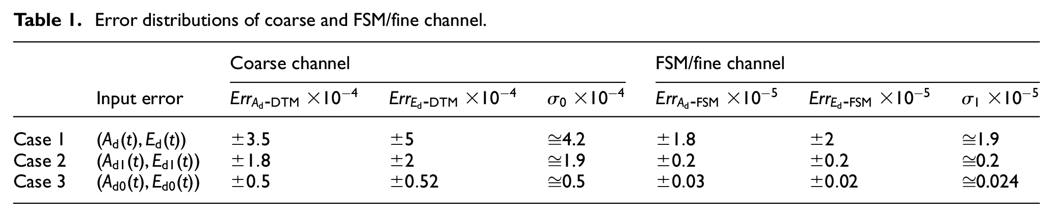
Firstly, for the coarse channel, Case 2 is the situation that filtered out high frequency pulsation caused by small scale high-frequency random perturbation vortices. Compared with the original input Case 1, the coarse channel accuracy is improved by about 2.21 times from 4.2 to 1.9. Moreover, compared with Case 2, Case 3 filters out the middle-frequency perturbation that could further improve the coarse channel accuracy to roughly 1.9/0.5 = 3.8 times.
Secondly, for fine channel, the corresponding improvement error times for composite tracking or FSM are about 1.9/0.2 = 9.5 and 0.2/0.024 = 8.3, respectively. This difference mainly relies on the narrow bandwidth of coarse channel. The distribution errors from medium scale vortices’ pressure pulsations have been significant improved by the coarse channel, which is about 3.8 times (Case 2 to Case 3) lager than 4.2/1.9 = 2.21 times (Case 1 to Case 2). However, for composite tracking, fine channel FSM supports a wider bandwidth appearing a better error compensation effect for random small scale, higher frequency pressure pulsation. Thus, the error enhancement time for high frequency from Case 1 to Case 2 is about 1.9/0.2 = 9.5 slightly larger than 0.2/0.024 = 8.3 from Case 2 to Case 3. But this comparison values for coarse channel are 2.21 and 3.8. It can be concluded that for a FSM offers 100–200 Hz bandwidth range, the error improvement capability is stronger for the introduction of small random perturbations with a frequency of 2–3 Hz or higher. During a new system’s design, more effort should be contributed on the selection of DC torque motor to catch the error at the middle frequencies.
Figure 17(a) to (c) show the azimuth and pitch angle tracking error density distributions for compound axis or FSM/fine channel tracking. It can be seen that the maximum density values of Figure 17(a) to (c) can reach to 1.6×10¹⁷, 8×10¹⁷, and 4.5×10¹⁹, respectively. Thus, for direction energy weapon, the control method in Figure 17(c) has a better control precision and laser destroying ability.
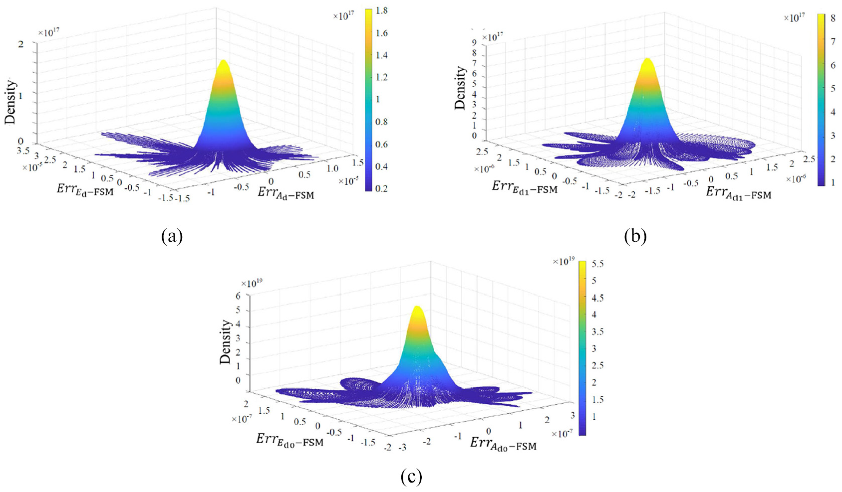
Three track density distributions for the fine tracking errors (a) Without mean-filter; (b) With high frequency filter; (c) With low-pass filter.
In general, through the simulation analysis, we can further obtain the disturbance characteristics and generation mechanism of multi-scale vortices as well as the corresponding pressure pulsation. Furthermore, the error compensation effects of coarse/fine channels for multi-scale pressure pulsation have been deeply investigated, providing more predictive guidance for the design of control system in practice.
Conclusions
Submarine hydrodynamic characteristics of 6° yaw angle underwater have been investigated in this investigation. Based on the vortices’ evolution, the relationships between the multi-scale pressure pulsation and output photoelectric servo tracking error have been numerical analyzed with its main conclusions as follows:
For submarine torque disturbance in high Reynolds number flow field, the influence of pressure pulsation plays a dominant role than the viscous force.
The fluctuations of middle/low frequencies are mainly caused by the boundary layer separation and shedding from the fluid flow around the submarine hull and appendage. High frequency random small perturbations mainly generated from the fluid’s random interaction as well as the energy exchange among different flow layers.
Pressure pulsations formed by different scale’s turbulence dissipative vortices are of difference impact on the error output of the tracking and targeting system. The coarse channel has more excellent performance on suppressing the middle scale pressure pulsation. While the FSM/fine channel has the best control effects for the high frequency small-scale pressure pulsation, it contributes more than the coarse channel, especially in complex flow environments.
The research on submarine’s fluid dynamics, including the inherent influence laws from the vertical/horizontal rudders and the propellers under different angles of attack needs further study. In addition, more accurate numerical methods and turbulence models will be adopted to provide a better and detailed view of the flow fluid. Moreover, the generating chaotic phenomena for the turbulence and distributions would be investigated, which are usually generated by non-linearities occurring in the examined system. The chaotic theories can help us to discuss the propeller distribution as well as detect the fine shadows from the propeller damage.
Footnotes
Declaration of conflicting interests
The author(s) declared no potential conflicts of interest with respect to the research, authorship, and/or publication of this article.
Funding
The author(s) disclosed receipt of the following financial support for the research, authorship, and/or publication of this article: This work is supported by the National Natural Science Foundation of China, NO. 11702139, and the Fundamental Research Funds for the Central Universities NO.30918014115-009.