
Abstract
In this paper, the propagation of uncertainty on a nonlinear measurement model is presented using a higher-order Taylor series. As the derived formula is based on a Taylor series, it is necessary to compute the partial derivatives of the nonlinear measurement model and the correlation among the various products of the input variables. To simplify the approximation of this formula, most previous studies assumed that the input variables follow independent Gaussian distributions. However, in this study, we generate multivariate random variables based on copulas and obtain the covariances among the products of various input variables. By applying the derived formula to various cases regardless of the error distribution, we obtained the results that coincide with those of a Monte-Carlo simulation. To apply high-order Taylor expansion, the nonlinear measurement model should be continuous within the range of the input variables to allow for differentiation, and be an analytic function in order to be represented by a power series. This approach may replace some time-consuming Monte-Carlo simulations by choosing the appropriate order of the Taylor series, and can be used to check the linearity of the uncertainty.
Introduction
In describing the propagation of uncertainty through a system, the first-order Taylor series is highly recommended by the Guide to the Expression of Uncertainty in Measurement (GUM). 1 However, it is difficult to accurately predict the uncertainty of a nonlinear measurement model using a first-order Taylor expansion. Thus, the GUM suggests adding higher-order terms of the Taylor expansion when the model cannot be represented linearly. The high-order terms are obtained from the second order Taylor expansion with the assumption that the input variables have normal distribution.
Monte-Carlo (MC) simulation is widely used for nonlinear measurement model since it can predict distributions as well as standard deviations of measurement model outputs. It is strongly recommended that sufficient number of simulations are required to achieve high accuracy of the estimation. For example, the GUM recommends a minimum of 200,000 simulations to obtain a 95% confidence. 2 Some simulations such as finite element method (FEM) numerical analysis, statistical parameter estimations, and complex signal processing often take hours to days.3–5 Therefore, in these cases, MC simulation is not suitable for the uncertainty propagation on the nonlinear measurement model. Various studies on uncertainty propagation have been conducted, and they are well summarized in Liu et al.,6,7 Meng et al., 8 and Ouyang et al. 9 Recent studies showed that the probability density function (pdf) of the output of the measurement model could be predicted even through the input has arbitrary distribution. Most studies, however, assume independent input variables or approximate by truncating high orders terms.
Recently, Wang and Iyer 10 added third-order terms to reduce the error produced by the truncation of the Taylor expansion, and showed that the uncertainty of the nonlinear measurement model could be predicted more accurately than using the technique recommended in GUM. Zhang extended the Taylor series to an infinite number of terms and proposed some methods to calculate the variance of the system. 11 Mekid and Vaja 12 calculated the uncertainty of the measurement model up to the third order using the skewness and kurtosis of the input variables. Xue et al. 13 derived the variances and covariances of the model based on the infinite expansion of the Taylor series. These approaches assume that the input variables are independent (or dependent) normal distributions, thus removing terms that are difficult to calculate analytically. Thus, they cannot be applied when the input variables do not obey a normal distribution and/or are correlated with each other.
In this paper, we re-derive the Taylor series for the covariance of a nonlinear measurement model regardless of distribution and correlation of the variables. We also show the method how to apply the derived formula to simple numerical simulation. In the numerical approach, we calculated the non-analytic terms in the formula (such as the covariance between products of input variables) from the multivariate random variables generated based on copulas. To obtain the partial derivatives of the system, an n-point stencil is applied across the multiple dimensions. As a result, the formula based on the higher-order Taylor expansion can be fully applied to covariance calculations on the nonlinear measurement model, irrespective of the distribution of the input variables.
This paper is organized as follows. In Section 2, the covariance of the nonlinear measurement model is re-derived using a Taylor series expansion. In Section 3, we show examples of applying the derived formula by simple numerical approach. Section 4 discusses the limitations of Taylor approximation, and Section 5 presents the conclusions to this study.
Theory
In probability theory and statistics, covariance is a measure of the degree of correlation between two random variables, x1 and x2. By applying the linearity of expectations, this can be represented as the “expected value of their product” minus the “product of their expected values.”
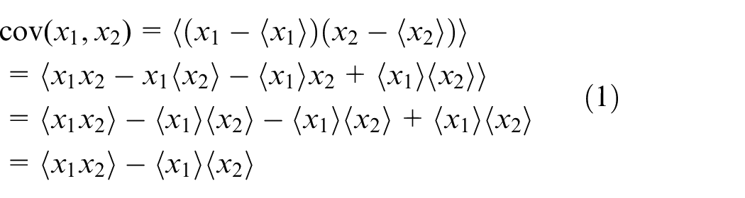
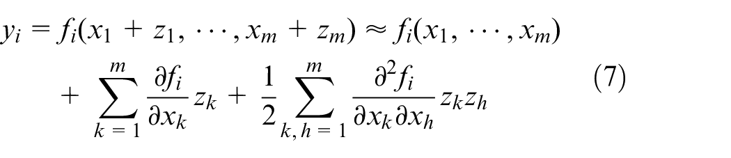
where 〈·〉 denotes the expectation of the argument. The approximate output of a system using the first-order Taylor expansion is
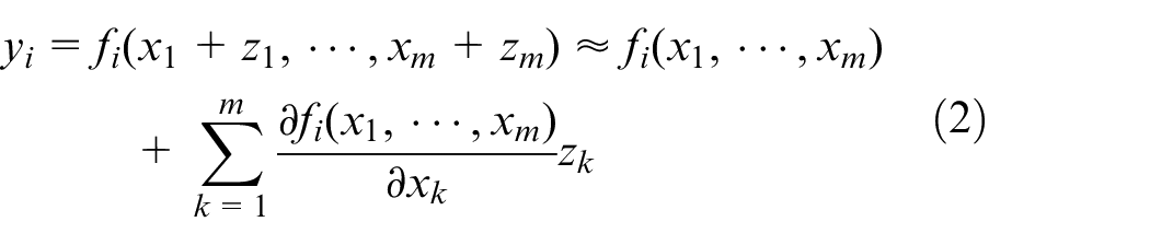
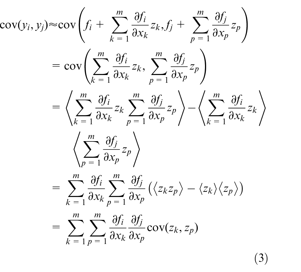
where xk is the input variable, zk is the error in xk, and y is the output of the function. f is a real-valued function that is differentiable on x1, …, xm; for simplicity, f(x1, …, xm) will be represented as f. Thus, the covariance using the first-order Taylor expansion is given by:
If there are m random variables, an m×m covariance matrix

The covariance matrix

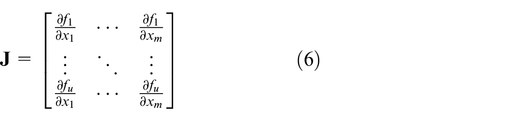
Here,
Equation (5), however, is not appropriate when the measurement model f is not linear. Thus, we require an accurate model for the nonlinear f and a method of propagating the uncertainty through it. In this paper, we use a higher-order Taylor expansion to obtain the covariance matrix of the nonlinear measurement model. It is not guaranteed that the covariance matrix will be expressed as a simple product of matrices, similar to equation (5). The approximation of the outputs using the second-order Taylor expansion is given by
The additive law of covariance is useful to simplify the Taylor expansion in equation (1).
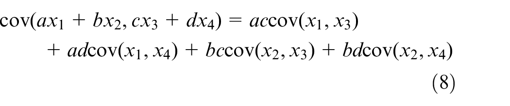
where a, b, c, and d are constants. Using equation (8), we can obtain approximations of the covariance of two outputs of the system:
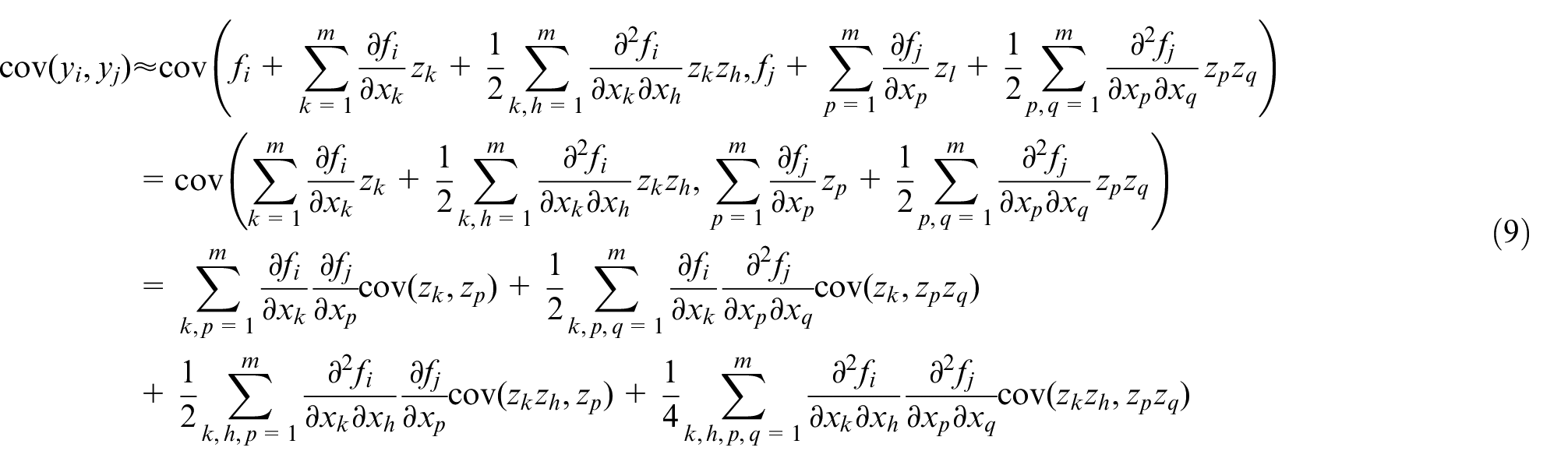
Similarly, the covariance of two outputs for the r-th order can be obtained based on the r-th order Taylor expansion.
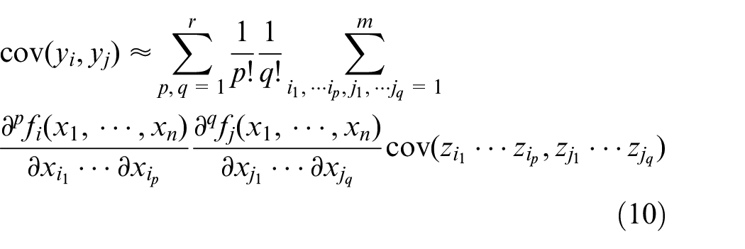
As a result, the covariance of the nonlinear measurement model can be represented as the covariance of the various products of input variables with their partial derivatives. Note that the analytic solution for the covariance of the product of variables has not known when they are not normal distribution. This makes equation (10) difficult to apply to the real problem. Equation (10), however, can be applied using a numeric calculation if we can compute the numerical partial derivatives and the numerical covariance for the product of input variables. We will show this in following section.
Numerical approach
As mentioned in the previous section, in order to apply equation (10), the partial difference of the measurement model and the covariance between the products of the input variables are required. There are various ways to find precisely the partial difference. In this study, we simply applied n-point stencil to focus on the applicability of the derived equation. It is beyond the scope of this paper to analytically calculate the covariance between the product of the input variables. Instead, we calculated it numerically and applied it to equation (10).
Numerical partial differentiation
The n-point stencil is widely used to obtain numerical derivatives. For example, the first partial derivative using a 5-point stencil is as follows:
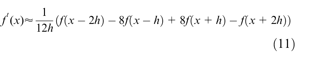
The n-point stencil can also be used to compute derivatives on the multivariable. However, we use a multi-dimensional m-point stencil to simplify the numerical implementation, as shown in Figure 1. For O variables, we require nO points. For the first-order partial derivatives, equation (11) is applied along each axis. As the order of the differentiation increases, such as for ∂2f/∂2x, equation (11) is modified appropriately; the formula can be found in Fornberg. 14 Note that this approach does not require additional induction to derive the appropriate formulas.
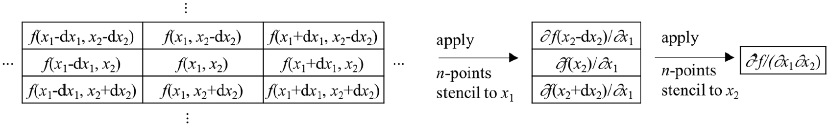
Multi-dimensional n-point stencil used in this paper.
Covariance of various products of input variances
Equation (10) requires the covariances of various products of input variables, such as
In applying the copula, multivariate normal random numbers are generated using Cholesky decomposition and converted to uniform random vectors. 17 These vectors are then transformed back to random numbers with the target marginal distributions using the inverse cumulative distribution function in MATLAB. 18 Depending on the marginal distribution, there may be a difference in the correlations between the target and the generated variables because of the nonlinearity of the transform. To overcome this issue, we apply Spearman’s ranked correlation. In a normal distribution, the Pearson correlation coefficient is related to Spearman’s rho as: 19
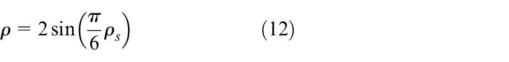
where ρs and ρ are Spearman’s and Pearson’s correlation coefficients, respectively. In this paper, to focus on the numerical approach, equation (12) is applied repeatedly until the generated random variables meet the target covariances. The detailed procedure is descried in the appendix.
Results
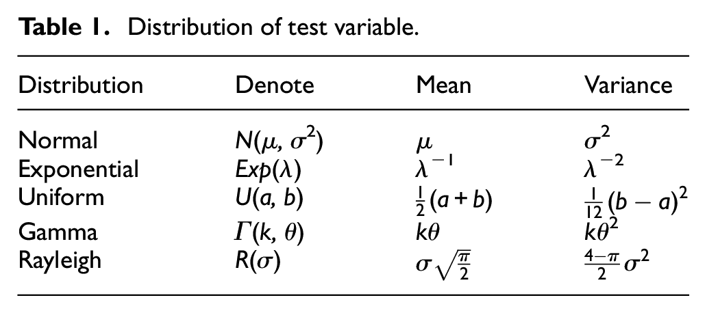
We tested the covariances of the nonlinear measurement model derived from the previous section using four nonlinear functions and five random variable distributions. The nonlinear functions are y1 = x13+x22+2, y2 = x12+x22, y3 = x12x2, and y4 = x1x2. The distributions considered here are the normal, exponential, uniform, gamma, and Rayleigh distributions; details are summarized in Table 1. We calculated the covariance of y1 and y2 and the covariance of y3 and y4 for the various distributions of input variables using a MC simulation and first-, second-, and third-order Taylor approximations. The MC simulations consisted of 1,000,000 runs; all results are summarized in Table 2.
Distribution of test variable.
Comparison of covariance using the MC simulation and the Taylor expansion.
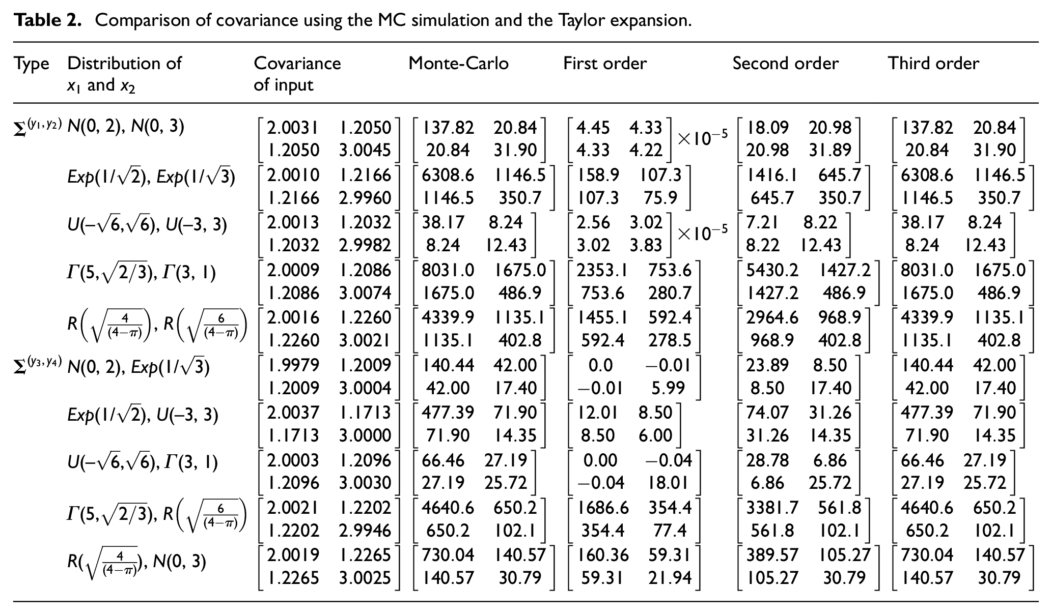
All random variables were generated to have the covariance matrix
Limitation of Taylor approximation
In this section, we study the limitation of the covariance based on Taylor approximation. The function f(x) = 1/(1 − x) is used as the nonlinear function. For the accuracy of calculation and convenience of analysis, the derivative of this function has been derived analytically and only one random variable is examined. The results of the Taylor series expansion of f are shown in Figure 2, where x = 2 and z = 0.9 and 1.01 (see equation (7)). For z = 0.9, the Taylor approximation converges to a value of 1/(1 − 2.9) when the differential order exceeds 40. For z = 1.01, however, the Taylor approximation diverges gradually. This is because the function f becomes discontinuous when the denominator is zero. Therefore, for the above function to be expressed as a Taylor series, the value of z should be between −1 and 1.
20
This corresponds well to the fact that the differentiable functions only can be represented as Taylor series. Figure 3 shows the variance of f as a function of the Taylor expansion’s order. When the variance of the input variable is 0.03, the variance of f using the proposed method approaches the result of the MC simulations (dashed line). However, it diverges from the MC simulation results for the case of 0.05, because the distribution of the random variable f(x) deviates from the continuous range, as shown in Figure 4(b). Therefore, the nonlinear measurement model approximating with the Taylor series should be a local continuous function that can be differential within the input variable range. It should also be an analytic function that can be expressed as the sum of the power series. Figure 3 additionally reveals that in the case of the measurement models that are difficult to describe mathematically, such as EVM and eye pattern measurement of complex signals,5,21 increasing the order of Taylor series and examining its convergence will be helpful in determining the differential order. Note that equations (9) and (10) show rapidly increasing number of calculation as the order of the Taylor series increase. For example, as the order increases to r, the amount of partial differential computation increases to
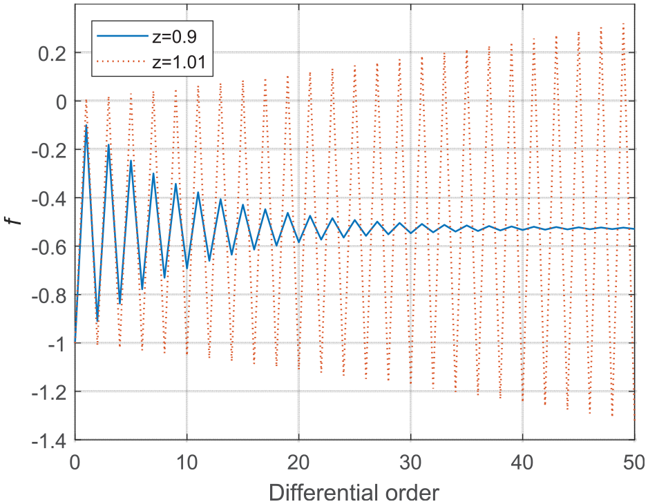
Taylor approximation for the output f.
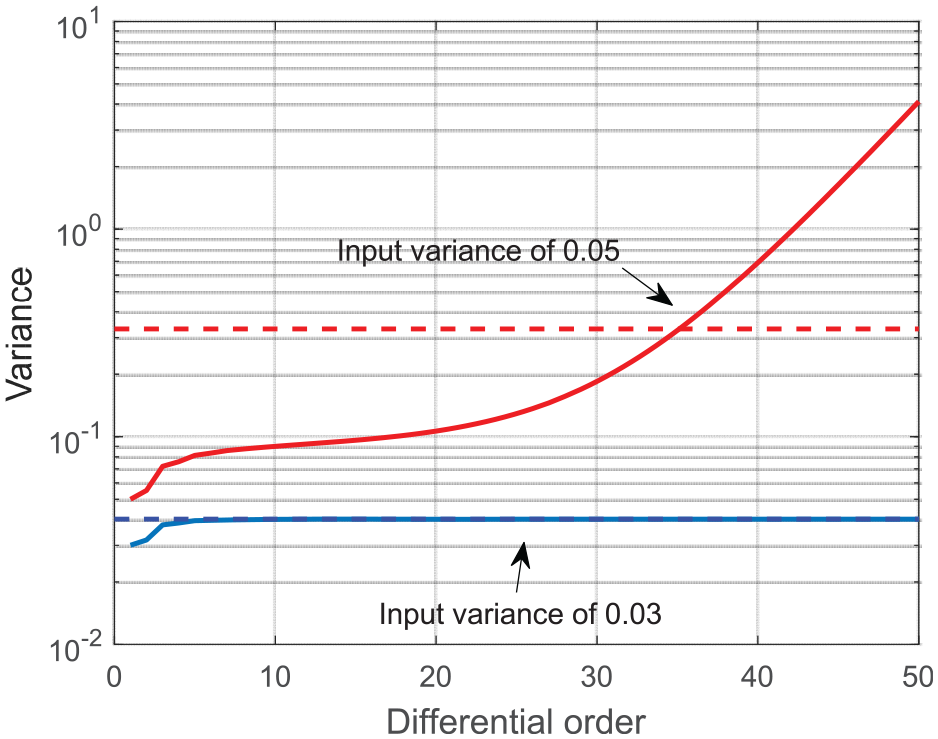
Taylor approximation for the variance of output.
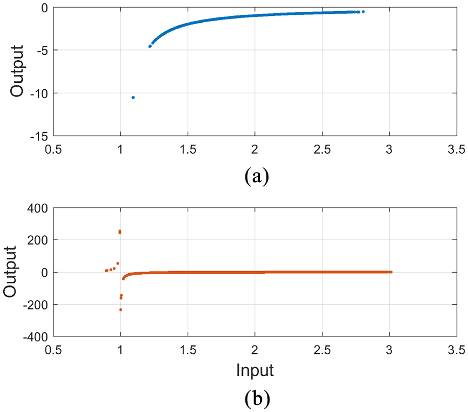
Input and output values in MC simulation: (a) for input variance of 0.03 and (b) for input variance of 0.05.
Conclusion
In this paper, we have re-derived a formula for estimating the covariances of nonlinear measurement model using high-order Taylor expansions. The presence of these high-order terms means that the expression is analytically intractable. Many previous studies have simplified these terms by assuming that the input variables obey normal distributions, whereas we generated multivariate random variables with arbitrary distributions and calculated these terms numerically. The estimation results were shown to be exactly the same as those given by MC simulations. We also showed that the nonlinear measurement model should be an analytic function that can be differentiated within the range of the input variables to apply high-order Taylor approximation.
The method used in Section 3 (Numerical Approach) may be used instead of time-consuming MC simulations such as the uncertainty evaluation on the finite element method (FEM) numerical analysis, statistical parameter estimations, and complex signal processing. It can also be used to evaluate the linearity of the uncertainty. This paper has focused on showing that the uncertainty propagation of nonlinear measurement model can be represented as high-order Taylor expansion and it can be applied in real problem using numerical approaches. Thus, it is left to the future studies that how to precisely generate multivariable random variables.
Footnotes
Appendix
Figure 5 shows the procedure and MATLAB code for generating multivariate random number used in both MC simulation and calculation of the covariance between products of input variables. First, the correlation coefficient CorCoeff is calculated by dividing the target covariance TargetCov by each standard deviation. Then, based on the calculated CorCoeff, multivariate numbers z having mean of 0 are generated. The generated z is then converted back into a uniform random vector u. In order to convert u back to a random number R with the desired target marginal distribution, we use MATLAB’s inverse cumulative distribution function (CDF) function. According to the inversion method, applying the inverse CDF of the distribution F to the uniform random variable U(0,1) produces a random number with exactly F distribution, which maintains the correlation coefficient of z. 22 If the covariance of the random number R is similar to that of TargetCov, these numbers are used both MC simulation and calculation of the covariance between product of input variables. If the difference of two covariance is large, apply equation (6) and repeat the above procedure. Thus, there are slightly differences between “covariance of input” and “Target covariance” as shown in Table 2.
Author’s note
Min-Hee Gu is now affiliated with Pixoneer geomatics.
Declaration of conflicting interests
The author(s) declared no potential conflicts of interest with respect to the research, authorship, and/or publication of this article.
Funding
The author(s) disclosed receipt of the following financial support for the research, authorship, and/or publication of this article: This research was supported by Physical Metrology for National Strategic Needs funded by Korea Research Institute of Standards and Science [KRISS-2019-GP2019-0005].