
Abstract
The existence of a Lyapunov function is known to ensure either local or global stability of a system’s equilibrium state. Inspired by the control-Lyapunov method, we here construct a Lyapunov candidate function by analyzing a pendulum system’s total energy and then applying appropriate control actions such that the conditions of a Lyapunov function are met. More specifically, our controller evaluates the Lyapunov function’s time derivative at each time step, and applies control torque such as to ensure that the Lyapunov function decreases for each step toward the goal upright state. Unlike the control-Lyapunov method, which aims to select control input as to minimize the Lyapunov function’s time derivative, our method provides up front the satisfactory conditions that yield a globally stable controller by using a rigorously designed proportional bang-bang control strategy. We show how to derive the controllers evaluation function, and how the controller is implemented in code. We further demonstrate the effectiveness of our method through numerical simulations. The result of our approach is a globally stable upright pendulum using a single-controller strategy.
Introduction
The simple pendulum and the cart-pendulum system’s are benchmark problems in the field of control. 1 These system’s are fairly simple to define yet non-trivial to control given their underactuated nature. Methods for locally and optimally stabilizing the inverted pendulum in the upright position are well established using linearized dynamics 2 and LQR. 3 In order to globally stabilize the inverted state, this local linear strategy is often paired with a swing-up controller.4,5 Another common and well established method is that of energy-pumping. 5 In this method, by pumping energy into the system, the system will continuously move to higher energy states. Among these is the state where the pendulum is inverted. This inverted state is however not an energy maximum as one can continue to increase the system’s energy infinitely beyond this point by increasing the system’s angular velocity. However, by switching control strategy to the locally linear method when the pendulum is close to inverted, the system can be made globally stable. This type of system thus requires two different controllers and a rule for when to switch between them, such as defining a switching boundary in state-space. The problem with such an approach is defining this state-space boundary, and the potential of chattering6,7 whenever the state is close to said boundary. In addition, such an approach also creates a discontinuous switch in control method which makes it more difficult to apply Lyapunov theory for proving global stability.
Given the potential downsides of multi-controller strategies, there is incentive to create a single-controller strategy that can yield global stability. Such methods have been explored in several instances. Shiriaev et al.8,9 inspired several subsequent methods by implementing a strategy based on energy considerations for the cart-pendulum. In their 19988 paper a discontinuous time-invariant state feedback was designed in order to achieve global attractivity of the upright position. In their 1999 9 paper the upright position was stabilized by means of continuous feedback, enabling almost all initial conditions be attracted to the upright position. David Angeli 10 extended the Shiriaev et al.8,9 papers and reported an almost globally stable method by adding positive and negative dissipation to the system. Srinivasan et al. 11 created a globally stable method by use of input–output linearization, energy control, and singular perturbation theory. Fujimoto and Sakamoto and Sakamato 12 formulated an optimal control problem including input saturation, and used the stable manifold algorithm to achieve global asymptotic stability and local exponential stability under actuator saturation. Magni et al. 13 used a model-predictive controller (MPC) with good results, however this method is more computationally expensive than the other approaches mentioned above. Aguilar-Ibañez et al. 14,15 used a Saturation Function Approach to make a cart-pendulum system globally stable in the upper half plane.
We present here a method for global inverted stability of the simple pendulum using a single-controller strategy. To the best of our knowledge, the approach is novel in its methodology and arguably simpler than many of the approaches seen previously. By not requiring switching between controllers we forego the mentioned downsides of a multi-controller strategy. We will be using the terms Lyapunov function and value function. A Lyapunov function has a strict definition as presented in section Lyapunov function’s below, while a value function is any function that assigns a single scalar value to a system state. In this paper, we will be creating a value function and turning this into a Lyapunov function by appropriate selection of actuation. Our method involves designing a value function which we turn into a Lyapunov function by selecting appropriate control values at each state. The method is inspired by the control-Lyapunov method, 16 but uses instead a single proportional bang-bang controller 17 evaluated on said value function which is known to yield good or even optimal results.
Lyapunov function’s
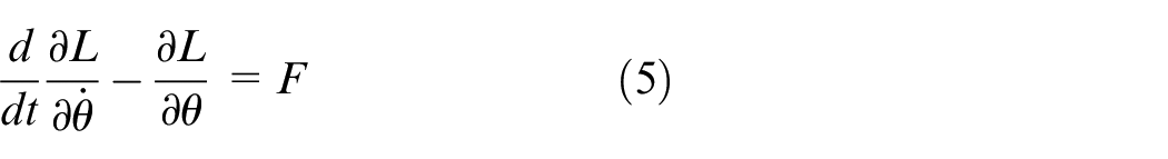
Lyapunov function’s are function’s that may be used to prove the stability of an ordinary differential equation’s (ODE) equilibrium. 18 For certain classes of ODEs, the existence of a Lyapunov function is a necessary and sufficient condition for stability. There is no general technique for constructing Lyapunov function’s for ODEs, but in some specific cases the construction of Lyapunov function’s is however known. One often well suited method for physical system’s is to construct a Lyapunov candidate function through conservation laws, such as the conservation of energy. 18 By definition a Lyapunov function is a scalar function that satisfies the following conditions:
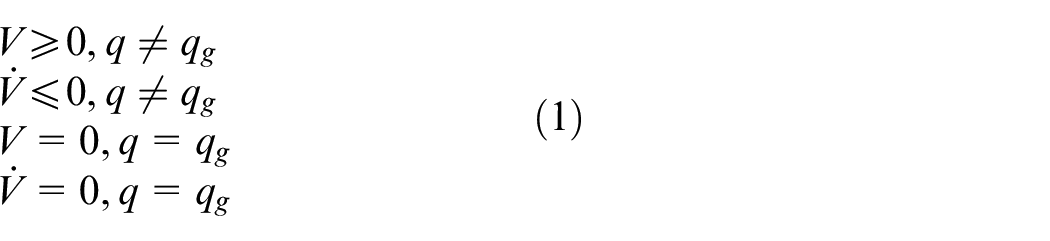
where

Here
Method
We will be using
The pendulum model
The system we will be working with is a classic benchmark system in underactuated control
1
; the underactuated inverted pendulum. As can be seen in Figure 1, the pendulum is comprised of a rod of length
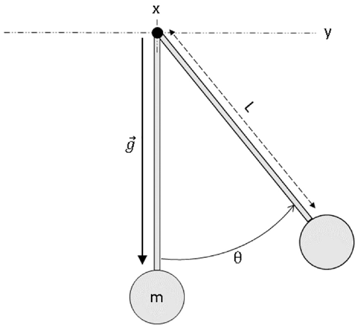
The simple underactuated pendulum.
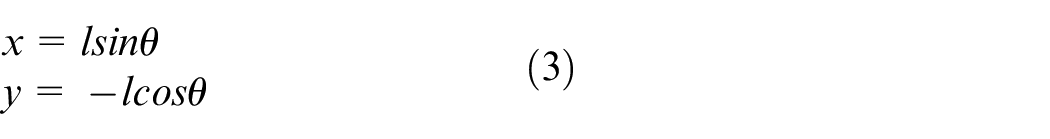
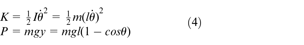
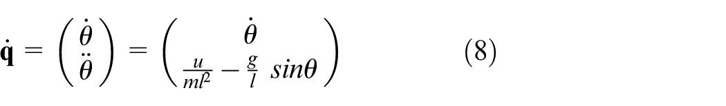
We derive the state-space model for this system by first defining the x and y coordinates of the point mass:
Since
It is easy to see that:
and
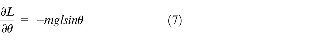
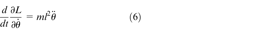
Plugging equations 6 and 7 into 5 and solving for
Defining V: a candidate Lyapunov function based on the system’s total energy
As mentioned earlier, for physical system’s a good strategy for creating a Lyapunov candidate function, in this case our value function, is to first define a suitable conservation law such as the system’s total energy. For our pendulum this energy is:
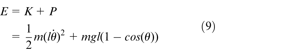
Here, the energy is the lowest when the pendulum is in the downright position with zero velocity
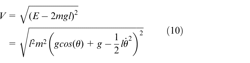
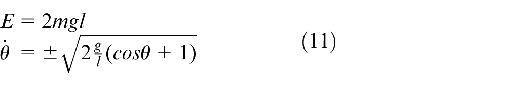
Now
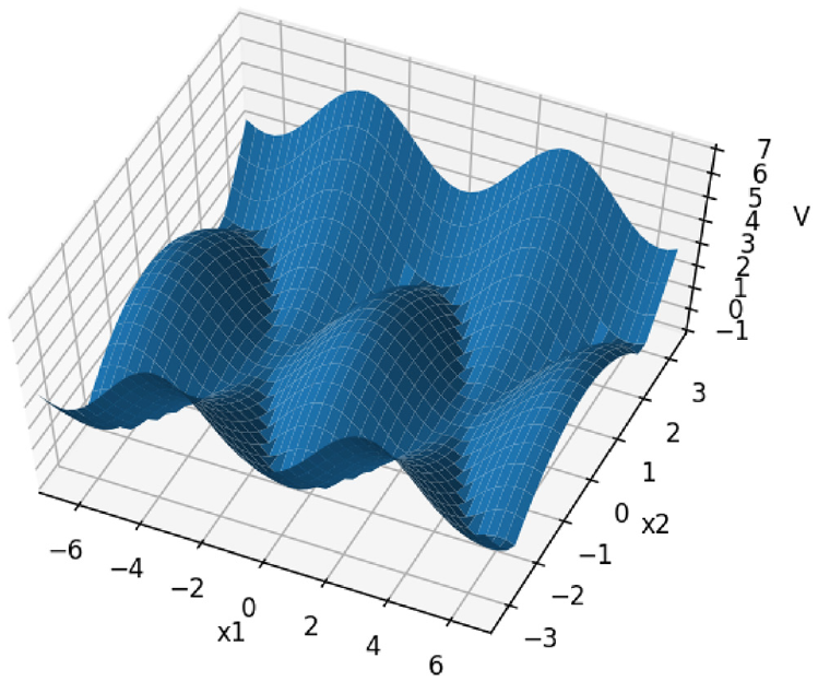
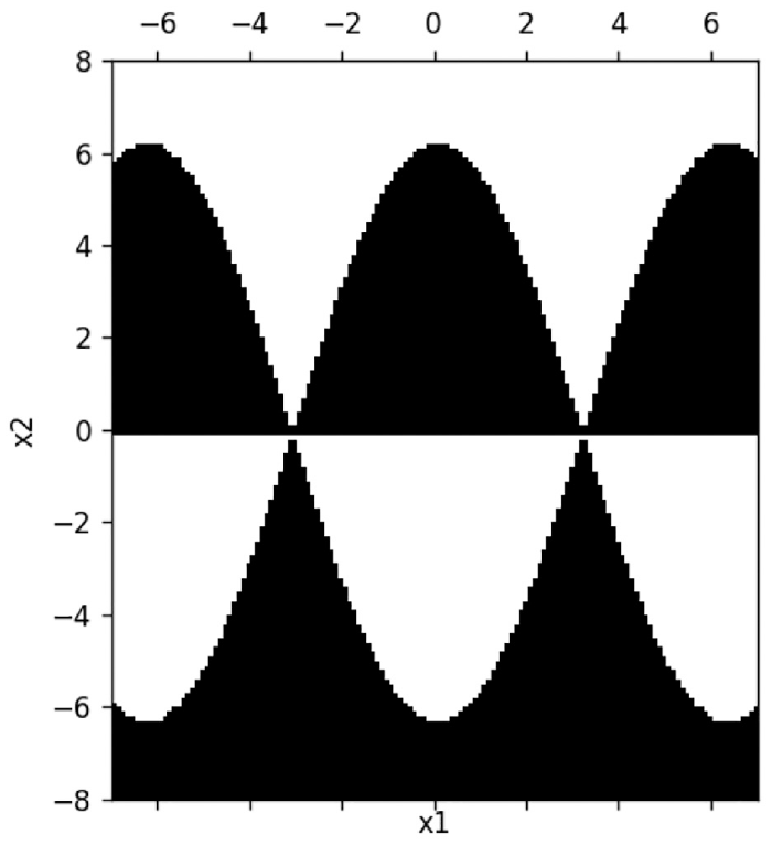
Plot of the value function
By creating a controller that is able to move the system state to these attractor lines from any initial state, it is possible to create a globally stable controller for the upright state.
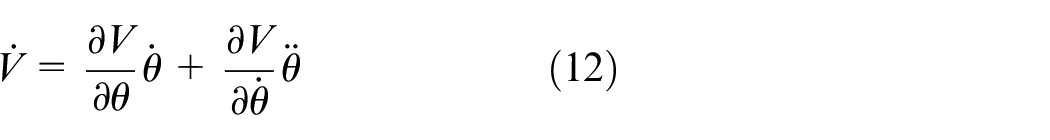
Defining V̇ and the control input u
We have now met our first condition for a Lyapunov function, which is to make
Using
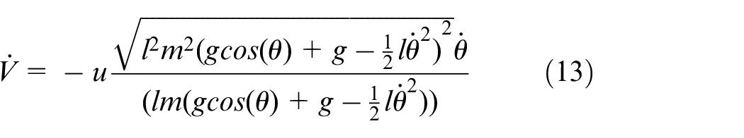
Now that we have an equation for
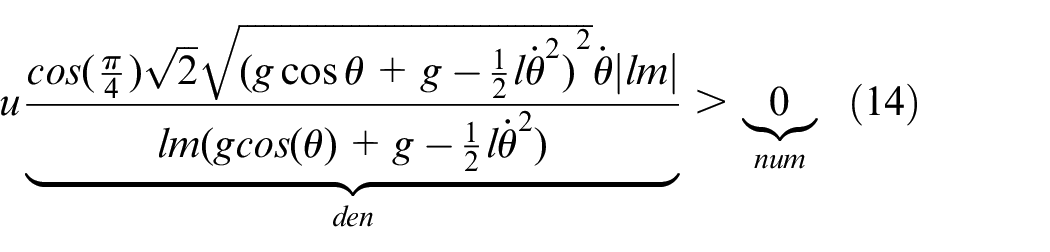
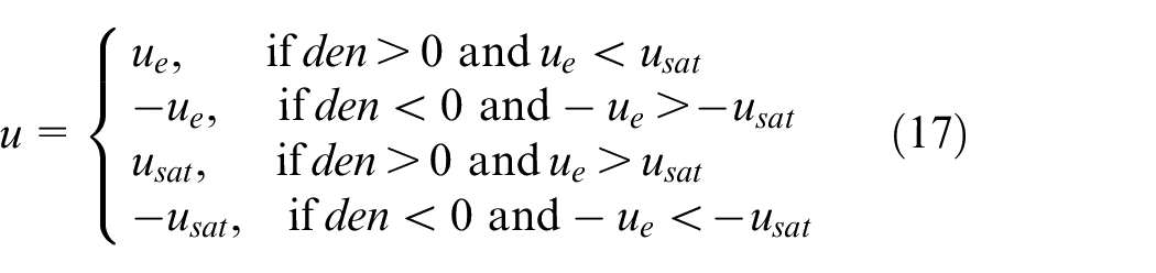
We see that the direction of the inequality sign is dependent on whether the left hand side denominator
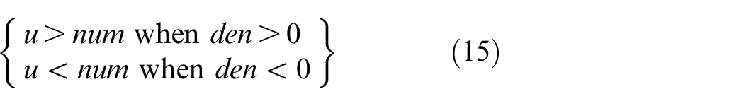
Figure 3 shows the selection of sign for u according to the above rule. We must further verify that this condition always holds such that we satisfy the conditions of equation 1, and to ensure the controller is true globally for the entire state-space. By simple inspection, we see that this condition is always satisfied as long as
Plot showing the the sign selection of
Creating a proportional controller
Pure bang-bang controllers that switch solely between maximum saturation values can cause chattering—undesirable high frequency control oscillations—which in turn can lead to a lot of wear on mechanical parts, as well as heat loss in electrical power circuits.
22
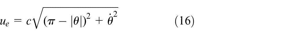
To circumvent this issue, we make our control input proportional to the Euclidean distance from the goal state
We implement this in the following Python example function:
Listing 1: Python function showing our bang-bang controller. The controller can be made proportional and takes the function den() as argument, which was found in equation 14. 0.75 is the proportional control constant c.
Results
We simulated our system in
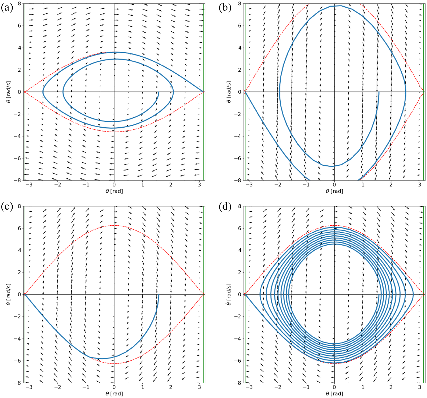
Simulations with parameters as presented in Table 1. The horizontal axes represent
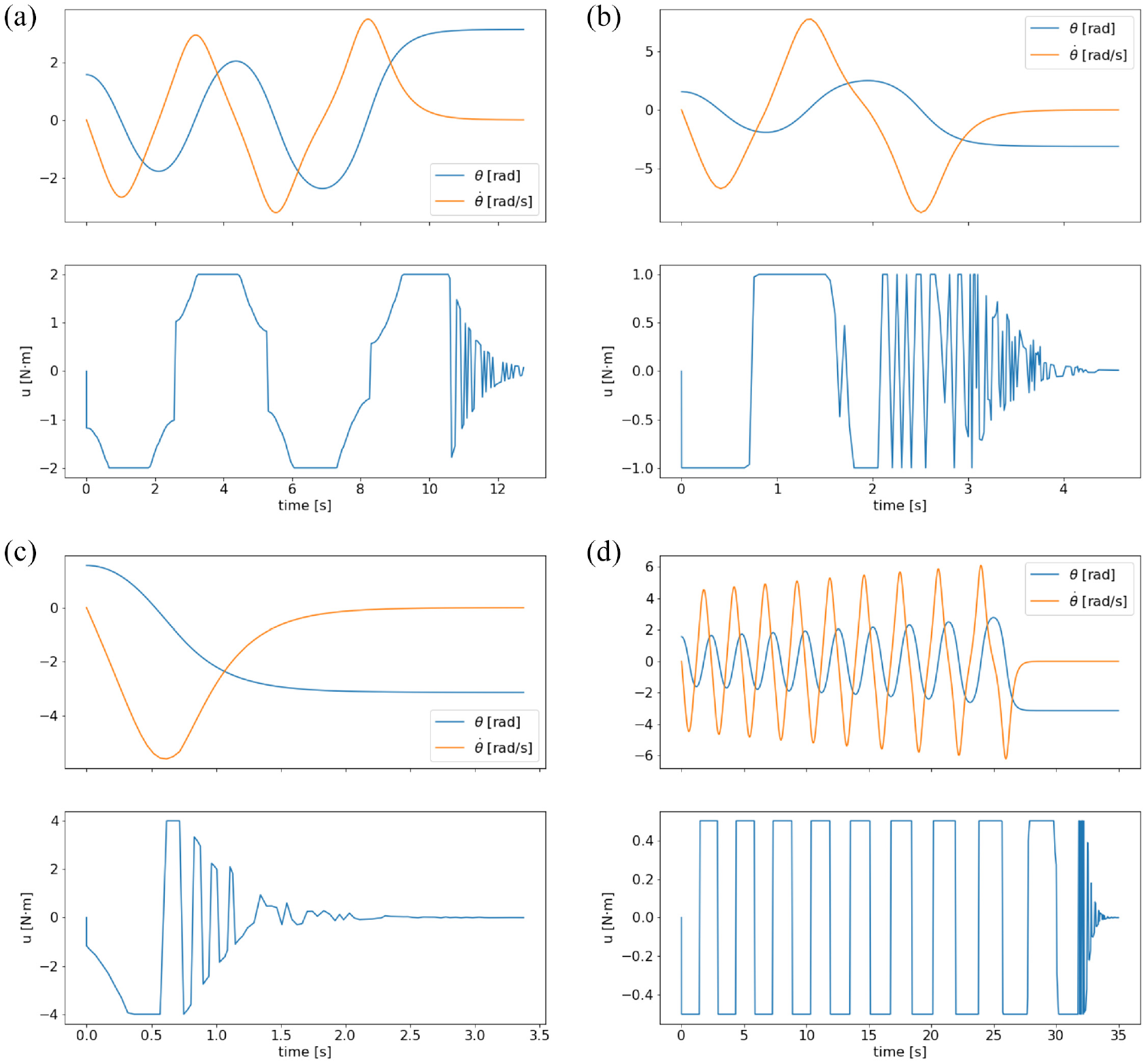
Simulations
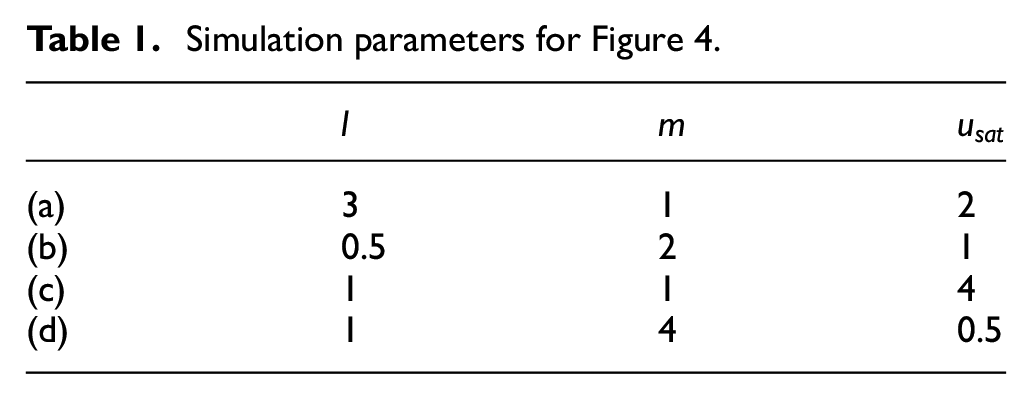
Simulation parameters for Figure 4.
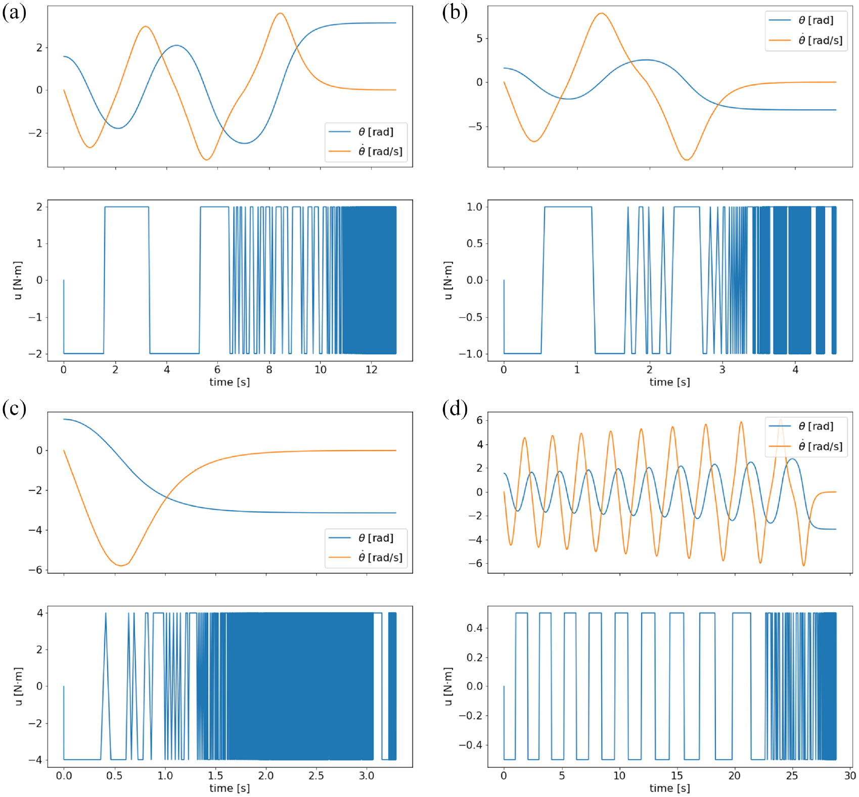
Comparing proportional control vs without
In Figure 6, we have performed the same simulation as in Figure 5, but without using the proportional part of the controller as in equation 17. As we can see, pure bang-bang control leads to considerable chattering which is alleviated with our proportional controller. Especially when we get close to the goal state, the pure bang-bang controller uses considerably more force than necessary to stabilize the inverted pendulum. This leads to constant chattering at this point
Simulations
Conclusion
We have here designed a proportional bang-bang control strategy which selects the sign of its control input by evaluating a modified energy derived value function. We have proved the conditions that need to be met by our saturated controller in order to make this value function a Lyapunov function as defined in section Lyapunov function’s. This was done by ensuring sufficient input torque as to satisfy the inequality 15. This also proved the controller to be globally applicable, since this condition is always satisfied as long as we have an
Footnotes
Declaration of conflicting interests
The author(s) declared no potential conflicts of interest with respect to the research, authorship, and/or publication of this article.
Funding
The author(s) disclosed receipt of the following financial support for the research, authorship, and/or publication of this article: The work was funded by The Department of Engineering Cybernetics, NTNU, Norway