Sage Journals: Discover world-class research

Abstract

In order to predict the remaining useful life (RUL) of rolling bearings in complex environmental conditions, a bearing RUL prediction method based on fractal dimension and one-dimensional convolutional neural network (1D-CNN) is proposed. This method uses fractal dimension to characterize the degeneration process of the rolling bearing and combines the features of time domain, frequency domain, wavelet packet domain, and entropy domain. Fractal dimension provides an analytical method for characterizing the complexity of vibration signals. The features extracted from different feature domains can complement each other’s advantages, reveal the degradation state of the bearing more comprehensively and achieve better performance. Then, the percentage of the remaining life of the bearing is used as the degradation tracking index of the rolling bearing. Based on the idea of stratified sampling, the training samples and test samples are constructed, and then a 6-layer CNN is constructed to train the model. Finally, three commonly used data sets of full-life bearings are used to verify the model, namely, IEEE prognostics and health management 2012 Data Challenge, IMS dataset, and XJTU-SY dataset. The experimental results show that, on the three experimental datasets, compared to the long short-term memory network (LSTM) and the extreme learning machine (ELM) methods, the prediction effect of the RUL of the bearing based on the fractal dimension and 1D-CNN proposed in our paper is better. Its mean absolute error and root mean square error (RMSE) and mean absolute percentage error (MAPE) have been reduced, and the correlation index (R²), adjusted_R², and relative accuracy (RA) have been improved, which can predict the RUL of the bearing more accurately.

Keywords

Remaining life prediction fractal dimension convolutional neural network degradation feature extraction

Introduction

With the continuous advancement of science and technology, machinery and equipment are increasingly developing in the direction of large-scale, precise, intelligent, automated, and systematic. In order to meet the needs of production, machinery and equipment are becoming more and more intelligent and complex. However, the working environment is often harsh and changeable. The equipment will gradually age after long-term operation, and the remaining useful life (RUL) will gradually decrease, thereby greatly increasing the potential for failure.¹ Driven by big data and artificial intelligence, research on fault prediction and prognostics and health management (PHM) technology has become more in-depth. This technology is not only traditional problem diagnosis, but also predictive performance analysis and intelligent maintenance of future states. Therefore, accurately predicting the RUL of the equipment is of great significance to the preventive maintenance decision-making of mechanical equipment.

Bearings are a key part of rotating electromechanical equipment, and their reliable operation can improve the safety and efficiency of modern production equipment. Generally speaking, bearings usually work in different environments, and different types of failures often occur during operation. If effective protective measures are not taken in time, it may cause the entire machine to malfunction and cause a lot of economic losses. Therefore, RUL prediction of bearings will be a very important task. It can provide early warning reports for equipment maintenance personnel and replace parts in advance, thereby reducing expensive unplanned maintenance and improving the safety of equipment operation.²

At present, the mainstream prediction methods of RUL mainly fall into three categories: prediction methods based on physical models, data-driven, and hybrid models.³⁻⁴ Essentially, these three methods can find applications in practical problems. However, the use of physical mechanisms and hybrid-based methods may be limited in practice, due to the lack of underlying physical knowledge in many practical components and systems. Remaining useful life prediction methods based on physical mechanisms generally have problems such as greater difficulty in modeling systems with higher complexity and lower universality of the established models on other systems. Because it is difficult to clearly and comprehensively describe the complex process of bearing degradation, data-driven can automatically infer hidden data. The causal relationship in the system directly extracts the degradation characteristics of the complex system, which can better process the massive monitoring data and provide accurate RUL prediction results.⁵⁻⁶ Generally speaking, the data-driven RUL prediction process includes three steps. First, different types of monitoring data, such as vibration or sound wave emission signals, are obtained through various sensors. Second, representative features are extracted from them using signal processing techniques, and then the selected features are input into Gaussian process regression,⁷ support vector machine (SVM),⁸ recurrent neural network (RNN),⁹ and other learning models to train the degradation behavior of the machine. Finally, these models are used to predict and estimate RUL.

With the continuous improvement of computer hardware level, deep learning^10,11 technology has received more and more attention in data-driven RUL prediction. Scholars have also conducted some research on machine RUL prediction based on deep learning. Kang et al.¹² used an improved sparse autoencoder to extract features, combined with a bi-directional LSTM (Bi-LSTM) to construct a prediction model, and estimate rolling elements Bearing RUL. Tian et al.¹³ developed a method based on artificial neural network (ANN) to achieve more accurate RUL prediction for state monitoring equipment, but the prediction results for small samples are not ideal. Sun et al.¹⁴ developed a RUL prediction model based on SVM and applied the model to bearing life prediction. The model is applied to the life prediction of bearings, and the results show that the model has high accuracy, but this method cannot extract the features needed to fully reflect the bearing degradation by using traditional feature extraction methods. Ren et al.¹⁵ proposed a deep learning method for predicting the RUL of multiple bearings by combining time domain and frequency-domain features. Cao et al.¹⁶ proposed a new deep prediction network-parallel multiple CNN with compression excitation mechanism and Bi-LSTM to integrate the entire network, using RUL prediction for rolling bearings. Han et al.¹⁷ tried to use the horizontal vibration acceleration signal and the vertical acceleration signal of the bearing to construct a one-dimensional CNN to realize automatic feature extraction. By setting the starting degradation point of the bearing sample, the RUL of the training sample is more accurate. Ding et al.¹⁸ proposed a stratified sampling which is different from the traditional time series data division method and applied to data division, in order to fully understand the data characteristics, use the fast Fourier transform to obtain the frequency characteristics from the original data, and use the mean square The root is used as the tracking metric; finally, a deep convolutional neural network model with no pooling layer composed of three convolutional layers and two fully connected layers is constructed. J. Yoo et al.¹⁹ developed a time-frequency image to construct a health index (HI) and used CNN to predict RUL. In order to improve the RUL prediction value, RNN,²⁰ AE, and bi-directional combined gated recurrent unit (Bi-GRU)²¹ have also been applied to the prediction of RUL bearings. CNN has also obtained excellent RUL prediction results due to its wide application and powerful feature extraction capabilities.

When rolling bearings are in different fault states, due to the difference in stiffness non-linearity, clearance, friction, and external load, different non-linear and non-stationary influencing factors are caused. These influences are reflected by vibration signals. How to extract effective fault features from the fault vibration signal is the key to fault diagnosis. The complexity of the geometric shape of the vibration signal of rolling bearings is related to the degree of non-linearity of the system. Fractal dimension provides an analysis method to characterize the complexity of the vibration signal. It can extract the state information of the equipment as a whole. It has been successfully applied in many fields.²²⁻²⁵ Fractal dimension is to characterize the irregularity and complexity of the fractal set at different scales. The fractal dimension obtained according to the fractal theory can describe the structural characteristics of the signal. Therefore, this paper takes fractal features into account in the extraction of the degradation characteristics of rolling bearings and combines the time-domain, frequency-domain, and time-frequency-domain features proposed in the previous literature²⁶ to better reflect the degradation state of the bearing.

The main tasks of this article are as follows:

1. Three commonly used data sets in the field of bearing failure health management, PHM 2012 challenge data set, IMS data set, and XJTU-SY data set were selected. Systematically analyze the bearing degradation information in these three data sets and deeply understand the degradation status of bearings under different environmental conditions.

2. Introduce the fractal dimension into the measurement to characterize the degradation of rolling bearings. Combine multiple feature domains such as time domain, frequency domain, wavelet packet domain, and entropy domain to extract the multi-dimensional fusion features of the original bearing. The percentage of remaining life is used as the tracking metric label of the training model.

3. The method of data stratified sampling is used to divide the training set and the test set, in which the length of the intercepted data is consistent with the dimension of the extracted features. The method of data stratified sampling can make the training model robust.

4. Construct a 6-layer CNN to fit the hidden mapping relationship between the degradation index and the multi-dimensional fusion features. CNN can automatically extract deep features. Due to its generalization and robustness, the prediction effect on other bearings is also better without changing the super parameters of the model.

The organization work of this article is as follows: The Preliminaries section introduces the basic knowledge of CNN structure and fractal dimension; the Experimental framework section explains the construction of the model and the evaluation indicators used in this article; the Experiment section presents the specific experimental results and analysis; The last section is the conclusion of this article and discusses future work.

Preliminaries

CNN structure

Convolutional neural network is a very popular deep learning framework model with powerful feature extraction capabilities and has been well applied in image recognition, natural language processing, and other fields. The weight-sharing network structure of CNN makes it more similar to a biological neural network, which reduces the complexity of the network model and reduces the number of weights. This advantage is more obvious when the input of the network is a multi-dimensional image, so that the image can be directly used as the input of the network, avoiding the complicated process of feature extraction and data reconstruction in traditional recognition algorithms.

Convolutional neural network mainly consists of three main components: convolutional layer, pooling layer, and fully connected layer. Generally, the convolutional layer and the pooling layer will appear in pairs. The neurons in the convolutional layer in CNN are only connected to certain neurons instead of connecting to all neurons. Local connection, weight sharing, and sub-sampling in space or time make the three structural characteristics of CNN. The more common CNN structure is shown in Figure 1.

Figure 1.

General convolutional neural network structure.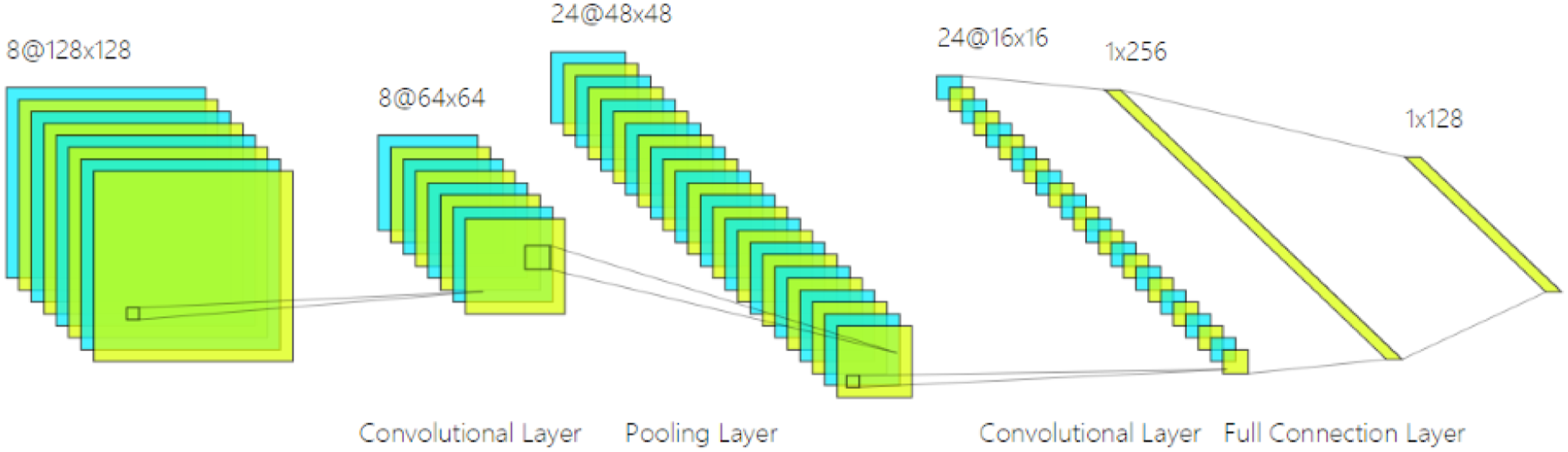

The function of the convolutional layer is to perform feature extraction by performing convolution operations on the local area of the input data and the convolution kernel, and to make the local receptive field traverse the entire input data by sliding the convolution kernel window. Each element that composes the convolution kernel corresponds to a weight coefficient and a bias, which is similar to the neuron of a feedforward neural network. Each neuron in the convolutional layer is close to the area of the previous layer. Each neuron is connected, and the size of the region depends on the size of the convolution kernel, which is called ”receptive field” in the literature.

The convolution formula is defined as follows

X_{i}^{(l + 1)} = f (W_{i}^{(l + 1)} * X^{(l)} + B_{i}^{(l + 1)})

(1)

X_{i}^{(l + 1)}

represents the (l + 1)th feature of the output value of the ith layer.

W_{i}^{(l + 1)}

represents the weight matrix of the ith convolution kernel of the (l + 1)layer,* represents the convolution operation, X ^(l) represents the output of the l-th layer, and

B_{i}^{(l + 1)}

represents the bias term. The function f represents the output activation function. CNN solves the non-linear problems in real life through the non-linear activation function. The commonly used activation functions are: Sigmoid, Tanh, and ReLU activation function.

The convolution process of CNN enables the convolution kernel to act on the feature area through a specified step size, thereby extracting new features. The weight of the same convolution kernel is the same, and different convolution kernels will get different outputs, and all outputs The features constitute the feature input of the next layer of pooling.

After feature extraction in the convolutional layer, the input features will be passed to the pooling layer for feature selection and information filtering. The pooling layer contains a preset pooling function, and its function is to replace the result of a single point of the feature map with the feature statistics of the adjacent area. The pooling layer selects the pooling area in the same steps as the scanning feature of the convolution kernel, which is controlled by the pooling size, step size, and filling. The role of the pooling layer is spatial merging or down sampling, which can reduce the dimension of the feature map while maintaining the most important signals. Generally, there are average pooling and maximum pooling; the expression for maximum pooling is as follows

y_{i}^{(l + 1)} = \max (x_{i}^{j} (k)), k \in D_{j}

(2)

y_{i}^{(l + 1)}

represents the element in the ith feature map of the (l + 1)th layer after pooling; D_j represents the j-th pooling area, and

x_{i}^{j} (k)

represents the element of the ith feature map of the lth layer in the range of the pooling core. The operation steps of maximum pooling is shown in the Figure 2.

Figure 2.

Max pooling.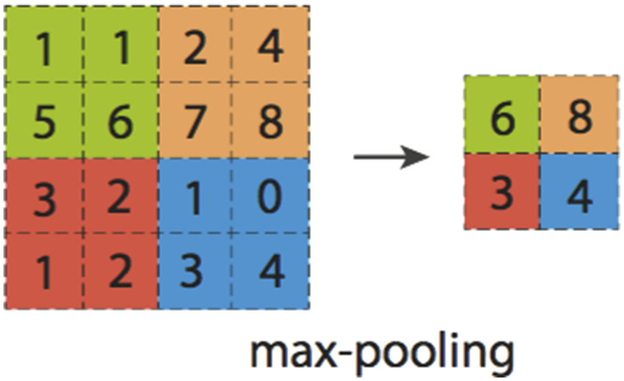

In the CNN structure, after multiple convolutional layers and pooling layers, one or more fully connected layers are finally connected. Each neuron in the fully connected layer is fully connected with all neurons in the previous layer. The fully connected layer can integrate the local information of the convolutional layer or the pooling layer.

Fractal dimension

Because the fractal dimension uses numerical methods to describe the fault characteristics, compared with the frequency spectrum method, the fault description is cleaner and more intuitive, and the amount of calculation is smaller.

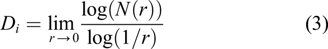
Fractal dimension is a parameter used to quantitatively describe the complexity and irregularity of an object. It can describe the object as a whole without relying on mathematical models. ²³ Therefore, the fractal dimension is an important feature of describing an object. At present, the more common fractal dimensions are box dimension, similar dimension, information dimension, correlation dimension, and generalized dimension. The box dimension is currently the most commonly used method for calculating the fractal dimension. Its calculation method is simple. The specific method is to cover the entire graph with small squares, and calculates the dimension by counting the number of all small squares covering the graph.The box dimension is specifically calculated by the following formula

D_{i} = lim_{r \to 0} \frac{\log (N (r))}{\log (1 / r)}

(3)

where N(r) represents the smallest grid count with the maximum diameter of r and that can cover the entire signal;

The size of the fractal dimension indicates the complexity and irregularity of the fractal object, and the larger the fractal dimension, the more complex the object and the more detailed components. Multifractal is a further extension of fractal theory. It uses a spectral function to describe the deeper and more detailed characteristics of the signal. With more in-depth research on fractal theory, scholars have found that only a single fractal cannot be described well. The more detailed characteristics of complex signals, and the generation of multifractals solves this problem.

Multifractal is not like a single fractal, which is a dimensional value. It is a collection of singularity measures of multiple scale indexes. Multifractal spectrum is usually used to express the relationship between the part and the whole.

The vibration signal of a rolling bearing is a non-linear and non-stationary signal. The fractal method is used to study it. Single fractal and multifractal are used to extract the characteristics of the rolling bearing vibration signal. Multifractal spectrum can more finely reflect the detail information contained in bearing signal and the degree of degradation information. The remaining life prediction is carried out by selecting the fractal box dimension and the multifractal spectrum corresponding to the original vibration signal as part of the degradation characteristics of the rolling bearing. The feature quantities extracted from the time domain, frequency domain, time-frequency domain, entropy domain, and fractal domain can complement each other’s advantages. Combining the features of multiple feature domains can reveal the degradation state of the bearing more comprehensively and achieve a more accurate remaining life prediction.

Experimental framework

In this section, all steps of the proposed RUL prediction method will be explained in detail.Our paper provide the whole sketch map of the proposed method as shown in Figure 3. First, extract 19-dimensional features from the fractal domain, time domain, frequency domain, wavelet packet domain, and entropy domain from the original vibration signal of the rolling bearing. Each feature can reflect the degradation process of the bearing throughout its life. Normalization processing can effectively avoid the impact of differences in the data itself. Then, the extracted 19-dimensional features are expanded into a one-dimensional vector in chronological order, where the first set of features represent the features extracted at the first sampling time, and the last set of features are the comprehensive features extracted at the last sampling time. CNN secondary feature extraction is performed on the unfolded one-dimensional vector, and the remaining percentage of the bearing is used as the tracking metric. The size of the convolution kernel of the first convolution layer is 19*1, and the step size is also 19, which means that each step The operation calculates 19 comprehensive features at the same time. The activation function uses the ReLU activation function, which can effectively avoid the insufficient gradient of the Sigmoid activation function or the insufficient gradient explosion. The maximum pooling layer is used to reduce the dimensionality of features, while not losing useful features as much as possible, and can greatly speed up training. Finally, two fully connected layers are connected to integrate the features after convolution and predict the final output result.

Figure 3.

Flowchart of the proposed method.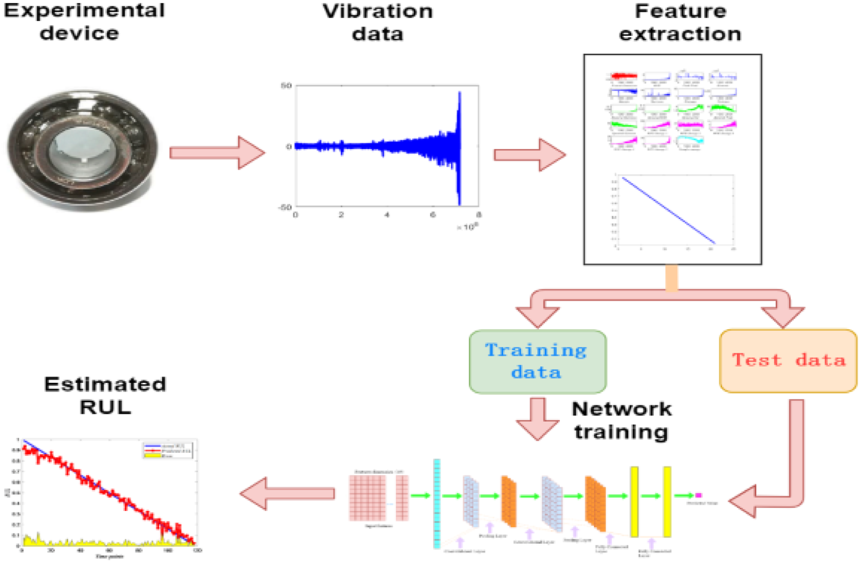

Bearing feature extraction

Time domain features and frequency-domain features can roughly reflect the decay process and fault information of rolling bearings. However, due to the non-linear characteristics of the bearing signal, the time-domain or frequency-domain features are very insensitive to non-linear components. When there are subtle changes, they cannot truly reflect their characteristics.

Wavelet packet decomposition is based on wavelet transform (WT), which can locally characterize the bearing signal characteristics. According to the research in Ref. 26, morlet is selected as the mother wavelet to extract part of the impact characteristics in the bearing, the number of decomposition layers is 4, and the first five normalized energies are used as time-frequency domain characteristic parameters.²⁶

In the entropy domain, the physical meaning of sample entropy and approximate entropy is roughly similar. They both measure the complexity of the time series by measuring the probability of generating new patterns in the signal. The greater the probability of a new pattern, the greater the complexity of the sequence. Compared with approximate entropy, sample entropy has two advantages: the calculation of sample entropy does not depend on the length of the data and sample entropy has better consistency, that is, changes in parameters m and r have the same effect on sample entropy. The lower the value of sample entropy, the higher the self-similarity of the sequence; the larger the value of sample entropy, the more complex the sample sequence. At present, sample entropy has applications in evaluating the complexity of physiological time series (EEG, sEMG, etc.) and diagnosing pathological conditions.

In the fractal domain, single fractal and multifractal are used to extract the characteristics of rolling bearing vibration signals. The multifractal spectrum can more finely reflect the detailed information contained in the bearing signal and the degree of degradation information. The remaining life prediction is carried out by selecting the fractal box dimension and the multifractal spectrum corresponding to the original vibration signal as part of the degradation characteristics of the rolling bearing.

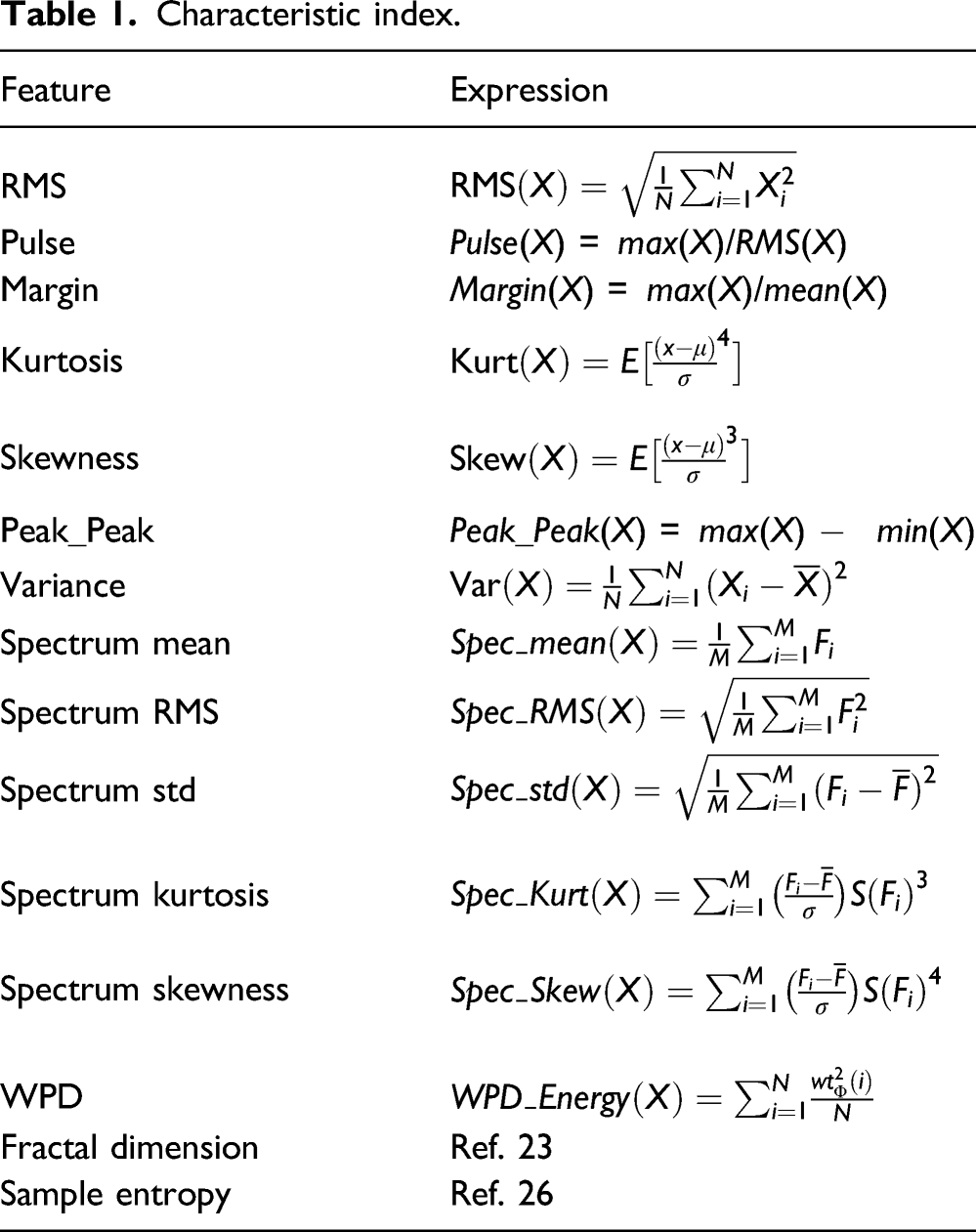
In the Table 1, X_i represents the original vibration signal, F_i represents the frequency spectrum after FFT, and S represents the standard deviation.

Table 1.

Characteristic index.

Feature	Expression
RMS	$RMS (X) = \sqrt{\frac{1}{N} \sum_{i = 1}^{N} X_{i}^{2}}$
Pulse	Pulse(X) = max(X)/RMS(X)
Margin	Margin(X) = max(X)/mean(X)
Kurtosis	$Kurt (X) = E [{\frac{(x - μ)}{σ}}^{4}]$
Skewness	$Skew (X) = E [{\frac{(x - μ)}{σ}}^{3}]$
Peak_Peak	Peak_Peak(X) = max(X) − min(X)
Variance	$Var (X) = \frac{1}{N} \sum_{i = 1}^{N} {(X_{i} - \bar{X})}^{2}$
Spectrum mean	$S p e c_m e a n (X) = \frac{1}{M} \sum_{i = 1}^{M} F_{i}$
Spectrum RMS	$S p e c_R M S (X) = \sqrt{\frac{1}{M} \sum_{i = 1}^{M} F_{i}^{2}}$
Spectrum std	$S p e c_s t d (X) = \sqrt{\frac{1}{M} \sum_{i = 1}^{M} {(F_{i} - \bar{F})}^{2}}$
Spectrum kurtosis	$S p e c_K u r t (X) = \sum_{i = 1}^{M} (\frac{F_{i} - \bar{F}}{σ}) S {(F_{i})}^{3}$
Spectrum skewness	$S p e c_S k e w (X) = \sum_{i = 1}^{M} (\frac{F_{i} - \bar{F}}{σ}) S {(F_{i})}^{4}$
WPD	$W P D_E n e r g y (X) = \sum_{i = 1}^{N} \frac{w t_{Φ}^{2} (i)}{N}$
Fractal dimension	Ref. 23
Sample entropy	Ref. 26

It can be seen from the above Figure 4 that the feature quantities extracted from the time domain, frequency domain, time-frequency domain, entropy domain, and fractal domain can complement each other. Starting from the characteristics of multiple feature domains, it can reveal the degradation state of the bearing more comprehensively, to achieve a more accurate remaining life prediction.

Figure 4.

Feature extraction map.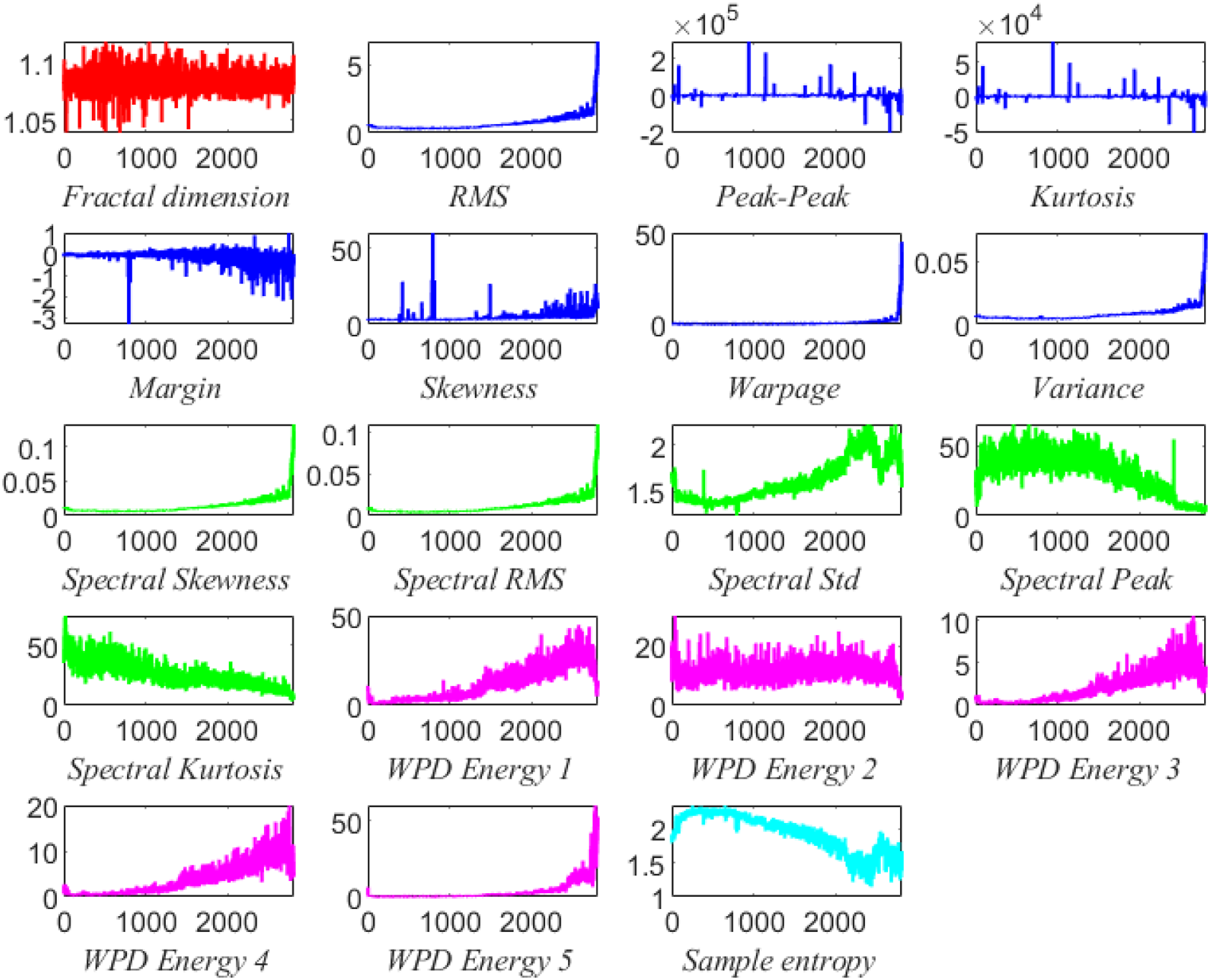

Percentage of Remaining Useful Life

Under normal operating conditions, the life of rolling bearings can reach thousands or tens of thousands of hours. However, running such a long time in a laboratory environment obviously does not conform to the actual conditions of the experiment. For the feasibility of the experiment, artificial methods are used to change the acceleration degradation process of the bearing. The main methods are to increase the speed of the rolling bearing, apply the extra load pressure of the rolling bearing, and reduce the use of lubricating oil. Therefore, the acquisition of bearing vibration signals is generally equal interval sampling.

For an experimental dataset, assuming that a total of n samples are taken during the experiment, the sampling frequency of the sensor is f, and the duration of each collection is s, then k (k = f*s) data are collected each time, If the sampling interval is m, the life of the bearing is n*m. Set the number of rows as the number of acquisitions, and the number of columns as the length of the data collected once.

For example, for the IMS data set, each bearing in the second set of experiments was collected 984 times, 20,480 data were collected each time, its life was 984*10 = 9840 min, a total of 164 h, the number of rows was set to be the number of times of collection, and the number of columns was the length of the data collected once.

Set the life label of the i-th row of data, which represents the ratio of the time from the time corresponding to the i-th row to the time when the bearing fails, and the ratio of the time from the start time of the bearing to the time when the bearing fails. Calculated as follows

y_{i} = \frac{n - i}{n - 1}

(4)

In formula (4), n is the number of rows currently in, and i is the total number of rows. The normalization of the life label can reduce the difference between different working conditions and different life values of the bearing, which is beneficial to improve the prediction accuracy of the RUL. Obviously, when the signal is first collected, the percentage of remaining life of the bearing is 1, and when the signal is finally collected, the percentage of remaining life of the bearing is 0.

Dataset division

Refer to the idea in the Ref. 18, using a stratified sampling method to divide the training set and the test set in order to better understand the entire degradation state of the data. The specific division steps are shown in the Figure 5. First, the extracted multi-domain features are expanded in a time series, and then extracted at a ratio of 19:1. The first 19 points of each group of data are taken as the training set, and the last point of each group of data is taken as test set. The advantage of dividing the training set and the test set in this way is to understand the degraded state of the bearing during the entire operation process and improve the accuracy of model training.

Figure 5.

Figure data stratified sampling method.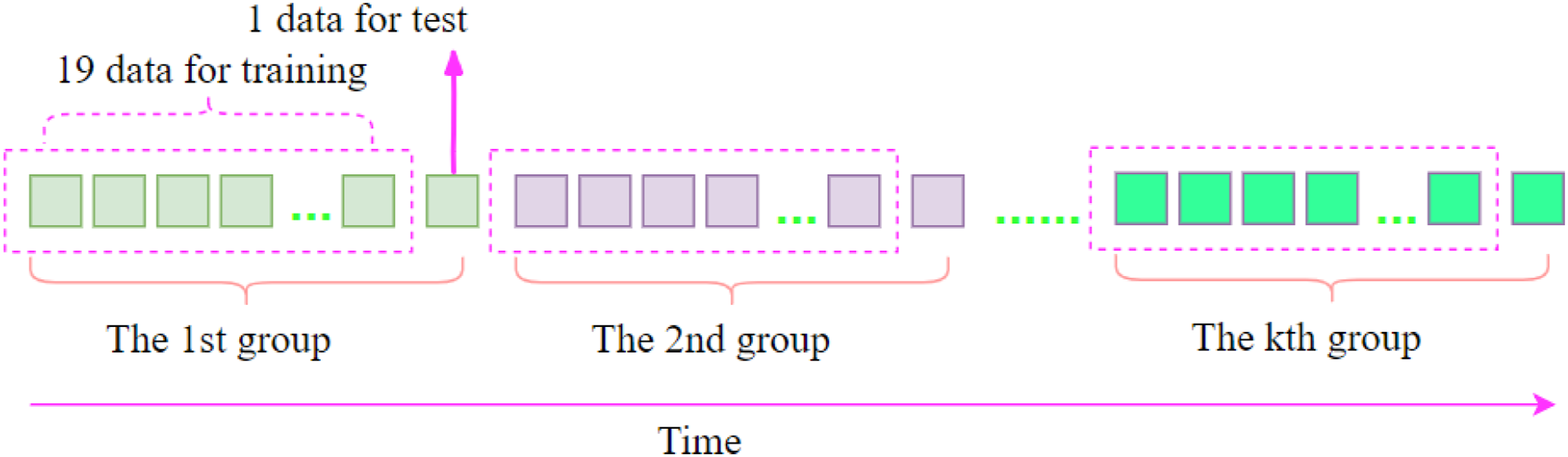

Evaluation index

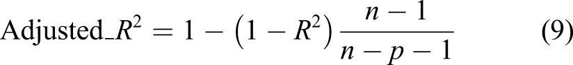
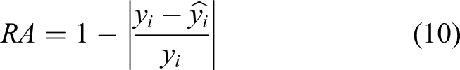
The following six indicators are used to measure the prediction effect of the proposed prediction model: mean absolute error (MAE), root mean squared error (RMSE), mean absolute percentage error (Mean), absolute percentage error (MAPE), and related indexes (R²),Adjusted_R². The calculation methods are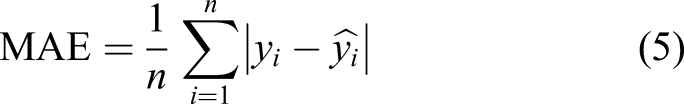

MAE = \frac{1}{n} \sum_{i = 1}^{n} | y_{i} - \hat{y_{i}} |

(5)

RMSE = \sqrt{\frac{1}{n} \sum_{i = 1}^{n} {(y_{i} - \hat{y_{i}})}^{2}}

(6)

MAPE = \frac{1}{n} \sum_{i = 1}^{n} | \frac{y_{i} - \hat{y_{i}}}{y_{i}} |

(7)

R^{2} = 1 - \frac{\sum_{i = 1}^{n} {(y_{i} - \hat{y_{i}})}^{2}}{\sum_{i = 1}^{n} {(y_{i} - \bar{y_{i}})}^{2}}

(8)

Adjusted_R^{2} = 1 - (1 - R^{2}) \frac{n - 1}{n - p - 1}

(9)

R A = 1 - | \frac{y_{i} - \hat{y_{i}}}{y_{i}} |

(10)

In formulas (5)–(10), $\hat{y_{i}}$ represents the predicted data, y_i represents the original acquired data, and n represents the length of the sampled data. Mean absolute error represents the error between y_i and $\hat{y_{i}}$ . RMSE reflects the error distribution, that is, the deviation between y_i and $\hat{y_{i}}$ . Mean absolute percentage error is used to measure the quality of a model’s prediction results. The smaller the three kinds of errors, the better the model. The correlation index R² is used to describe the effect of fitting. The larger of the R², the better the fitting effect of the model.

In order to avoid the excessive influence caused by the error caused by the excessive number of data samples, the adjusted R² is used to estimate the correlation index, where n represents the number of sample data, and p represents the dimension of the data feature. The relative accuracy (RA) definition is used to measure the difference between the predicted value and the true value. The result is between 0 and 1. The closer to one, the better the result.

Experiment

Experimental dataset

Under normal operating conditions, the life of rolling under normal operating conditions, the life of rolling bearings can reach thousands or tens of thousands of hours. However, running such a long time in a laboratory environment obviously does not conform to the actual conditions of the experiment. For the feasibility of the experiment, the accelerated degradation process of the bearing is changed by manual methods. The main method is to increase the speed of the rolling bearing, apply the additional load pressure of the rolling bearing and reduce the use of lubricants. The effectiveness of the method proposed in this paper is verified by using three experimental data sets.

1. FEMTO-ST bearing dataset(IEEE PHM 2012)

The first data set selected for the experiment comes from the PHM data challenge held by the Institute of Electrical and Electronics Engineers (IEEE) in 2012.²⁷ It is the vibration acceleration data collected from the rolling bearing accelerated life test bench (PRONOSTIA). The experimental platform is dedicated to It is an experimental platform for testing and verifying data-driven rolling bearing failure, degradation state assessment and remaining service life prediction. The acceleration sensor collects vibration information in the horizontal and vertical directions. The experiment set the condition for the complete degradation of the bearing to be that the amplitude of the vibration signal is greater than 20 g. The specific working condition information of the experimental platform is shown in the Table 2.

Table 2.

PHM bearing test condition information.

Condition	Rotating Speed(rpm)	Load(N)	Data file
Condition 1	1800	4000	1_1.1_2.1_3.1_4.1_5.1_6.1_7
Condition 2	1650	4200	2_1.2_2.2_3.2_4.2_5.2_6.2_7
Condition 3	1500	4500	3_1.3_2.3_3

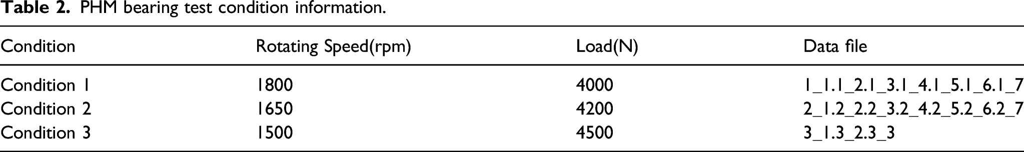
The experiment set up three different working conditions, of which the first and second working conditions have seven bearings, and the third working condition has three bearings. A total of the lateral vibration signals and longitudinal vibration signals of these 17 bearings during the entire service life are collected. Here, the horizontal vibration signals are selected for the experiment. The sampling frequency of the data is 25.6k Hz, and the data is recorded every 10 s, the length of each recording is 0.1 s, and the length of data collected each time is 2560.

For example, bearing1_2 has collected 871 times, 2560 data each time, its life span is 871*10 = 8710 s, set the number of rows as the number of collections, and the number of columns as the length of the data collected once.

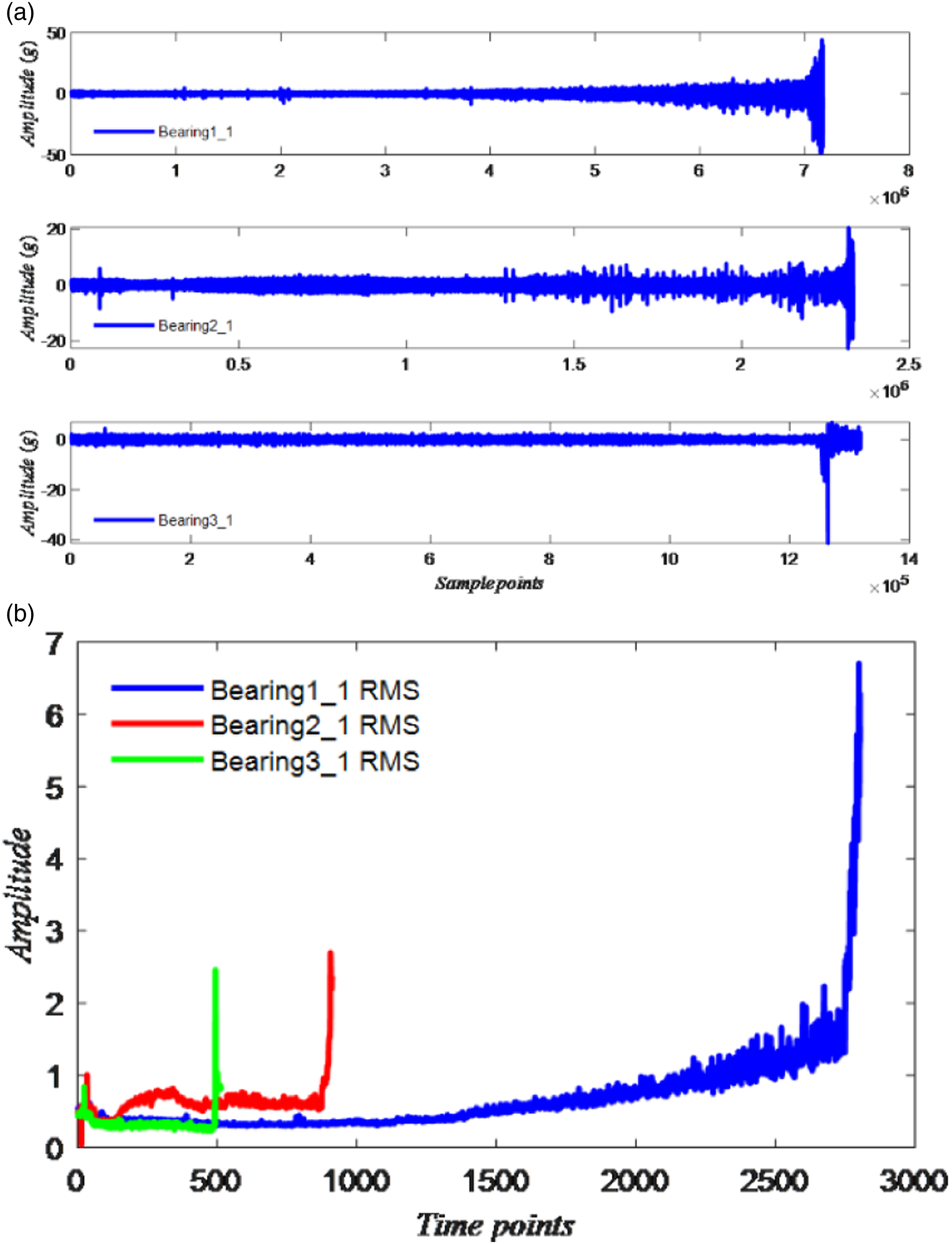
The original vibration signals of rolling bearings under three different working conditions and the corresponding root mean square values are shown in the Figure 6. It can be seen that under the three working conditions, the degradation degree and degradation process of each bearing are different.

2. IMS dataset

Figure 6.

Prognostics and health management bearing data information. (a) Raw vibration signal of the prognostics and health management bearing 1_1, 2_1, 3_1. (b) RMS of the prognostics and health management bearing 1_1, 2_1, 3_1.

The second set of rolling bearing life cycle data comes from the University of Cincinnati, Intelligent Maintenance System (IMS).²⁸ There are a total of four bearings, the acceleration vibration signal is measured, the sampling frequency is 20 kHz, the sampling period is 10 min and each sampling time is 1s, so the number of collection points each time is 20 480. The specific working condition information of the experimental platform is shown in the Table 3. Based on the principle of the amount of debris absorbed by the magnetic screw plug in the tubing, when the preset threshold is reached, the bearing can be considered to be degraded and the collection work is stopped.

Table 3.

IMS bearing test bed condition information.

Information	First group	Second group	Third group
Bearing number	B1,B2,B3,B4	B5,B6,B7,B8	B9,B10,B11,B12
File description	2156 files in total	984 files in total	4448 files in total

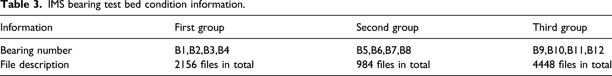
This paper selects the vibration acceleration signals of the four rolling bearings in the second set of experiments in the database as the signal data of the full life of the bearing. Each bearing in the second set of experiments is sampled 984 times, and the data is sampled every 10 min, and the sampling time is 1s each time., The sampling frequency is 20 kHz, so the number of acquisition points each time is 20 480, and the outer ring fault frequency is 236.4 Hz. The original vibration signals of rolling bearings under three different working conditions and the corresponding root mean square values are shown in the Figure 7.

3. XJTU-SY dataset

Figure 7.

Intelligent Maintenance System bearing data information. (a) Raw vibration signal of the Intelligent Maintenance System bearing 1,2,3,4. (b) RMS of the Intelligent Maintenance System bearing 1,2,3,4.

The third data set selected for the experiment comes from XJTU-SY data set.²⁹ The dataset contains the full-life cycle vibration signals of 15 rolling bearings under three working conditions. This experimental platform is shown in the figure below, which is mainly composed of AC motor, motor speed controller, rotating shaft, support bearing, hydraulic loading system and test bearing. The specific working condition information of the experimental platform is shown in the Table 4. In the experiment, the sampling frequency is set to 25.6 kHz, the sampling interval is 1min, and the duration of each sampling is 1.28 s, that is, the number of sampling points each time is 32 768. The original vibration signals of rolling bearings under three different working conditions and the corresponding root mean square values are shown in the Figure 8.

Table 4.

XJTU-SY bearing test bed condition information.

Condition	Rotating Speed(r/min)	Load(kN)	Data file
Condition 1	2100	12	1_1.1_2.1_3.1_4.1_5
Condition 2	1650	11	2_1.2_2.2_3.2_4.2_5
Condition 3	1500	10	3_1.3_2.3_3.3_4.3_5

Figure 8.

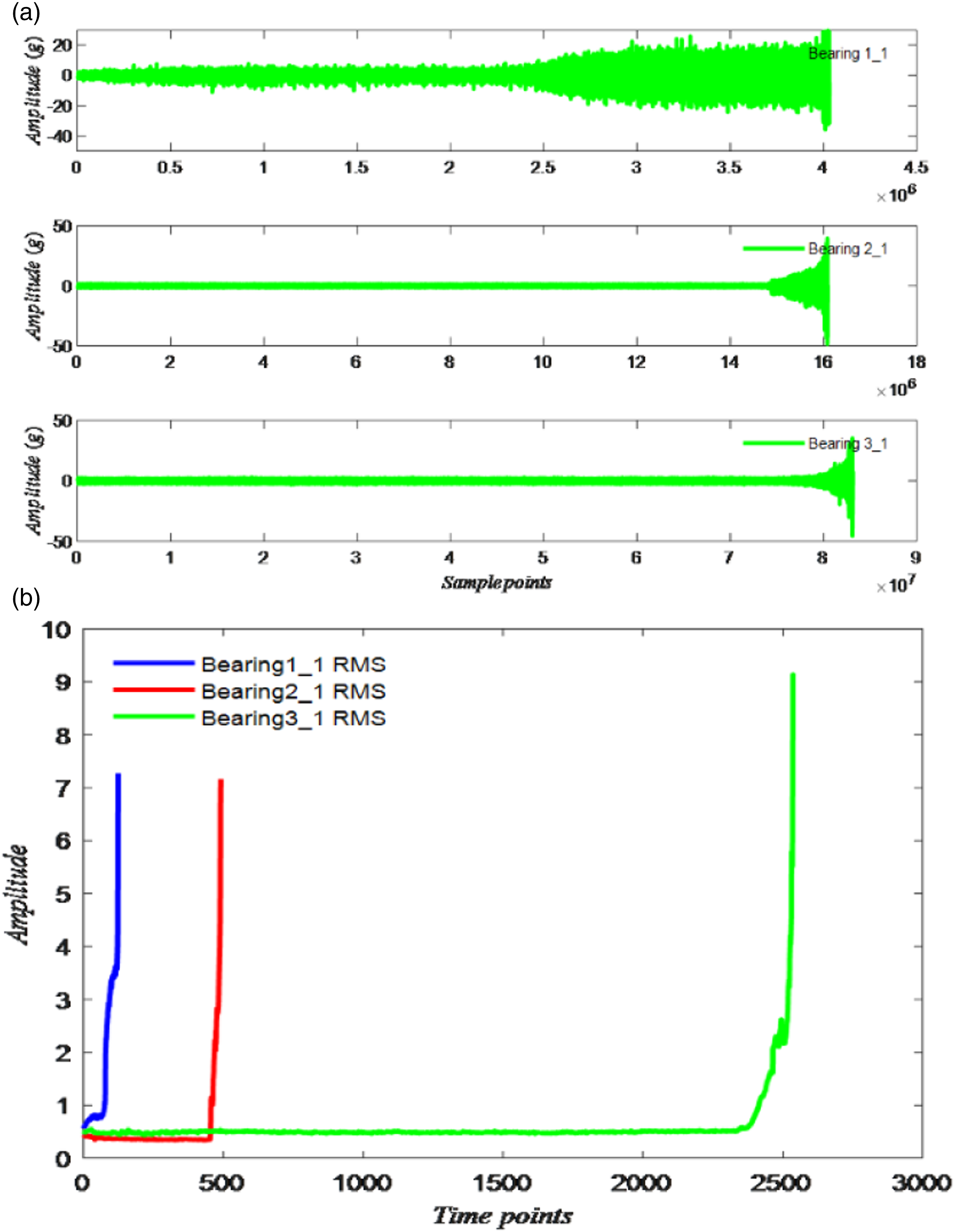
XJTU-SY bearing data information. (a) Raw vibration signal of the XJTU-SY bearing 1_1.2_1.3_1. (b) RMS of the XJTU-SY bearing 1_1.2_1.3_1.

The abscissa of the bearing in the three working conditions of the PHM data set represents the time point of the bearing operation; the interval between each time point is 10 s; the ordinate is the value corresponding to the RMS at different time points. The analysis shows that the degradation trend of each bearing varies with the running time, which indicates that the degradation trend of the four bearings is different. The sampling interval of the IMS data set is 10 min. The sampling interval of the XJTU-SY data set is 1 min. The sensor sampling frequency and sampling time interval of the three experimental data sets are not the same, so that the complex situation in the actual working conditions can be better reflected.

Experiment procedure

A CNN model is constructed to estimate the RUL. The hidden hyperparameters of CNN are robust. This CNN structure has six layers, including two convolutional layers, two maximum pooling layers, and two fully connected layers. The specific structure of the network is shown in Figure 9. The experiment was carried out using Windows 10 system, and the central processing unit (CPU) used the 1.80 GHz i5 processor internal storage to be 8.0 GB, and the real test software was used. The version of MATLAB R2019a was used for the experiment.

Figure 9.

Structure of convolutional neural network.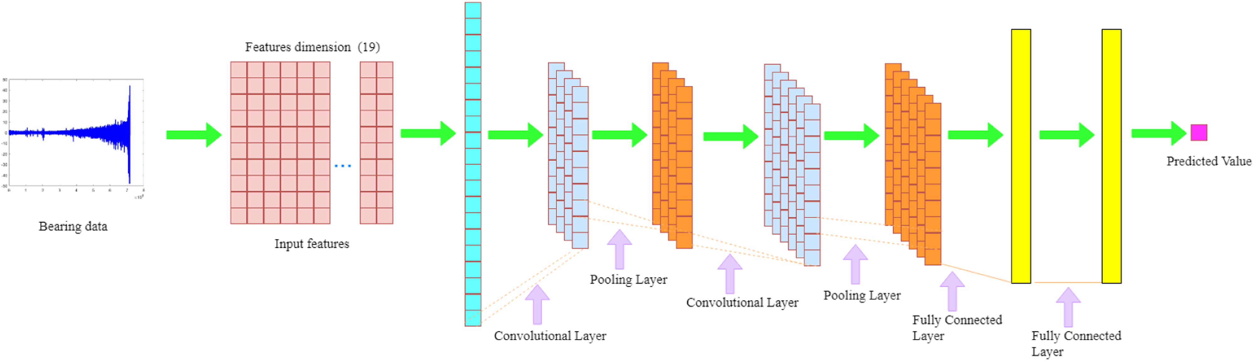

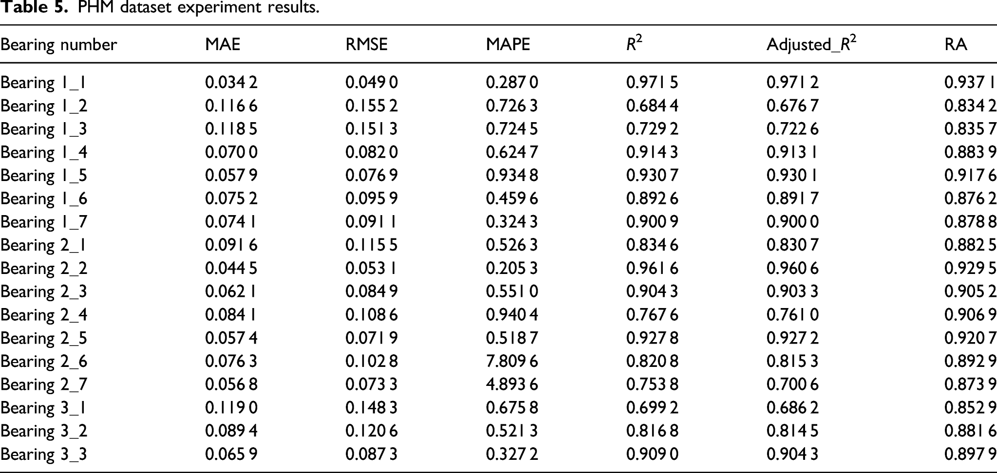
In the experimental process, the data of each incoming CNN network structure is normalized to a 19-dimensional feature. In the process of training CNN, MSE is used as the loss function of the training CNN, Adam optimizer is used, and the number of iterations is 200.^18,19 The experimental verification is carried out by the method of leaving one, and the results of six evaluation indicators of the three data sets obtained by the test are shown in the Tables 5–7.

Table 5.

PHM dataset experiment results.

Bearing number	MAE	RMSE	MAPE	R ²	Adjusted_R²	RA
Bearing 1_1	0.034 2	0.049 0	0.287 0	0.971 5	0.971 2	0.937 1
Bearing 1_2	0.116 6	0.155 2	0.726 3	0.684 4	0.676 7	0.834 2
Bearing 1_3	0.118 5	0.151 3	0.724 5	0.729 2	0.722 6	0.835 7
Bearing 1_4	0.070 0	0.082 0	0.624 7	0.914 3	0.913 1	0.883 9
Bearing 1_5	0.057 9	0.076 9	0.934 8	0.930 7	0.930 1	0.917 6
Bearing 1_6	0.075 2	0.095 9	0.459 6	0.892 6	0.891 7	0.876 2
Bearing 1_7	0.074 1	0.091 1	0.324 3	0.900 9	0.900 0	0.878 8
Bearing 2_1	0.091 6	0.115 5	0.526 3	0.834 6	0.830 7	0.882 5
Bearing 2_2	0.044 5	0.053 1	0.205 3	0.961 6	0.960 6	0.929 5
Bearing 2_3	0.062 1	0.084 9	0.551 0	0.904 3	0.903 3	0.905 2
Bearing 2_4	0.084 1	0.108 6	0.940 4	0.767 6	0.761 0	0.906 9
Bearing 2_5	0.057 4	0.071 9	0.518 7	0.927 8	0.927 2	0.920 7
Bearing 2_6	0.076 3	0.102 8	7.809 6	0.820 8	0.815 3	0.892 9
Bearing 2_7	0.056 8	0.073 3	4.893 6	0.753 8	0.700 6	0.873 9
Bearing 3_1	0.119 0	0.148 3	0.675 8	0.699 2	0.686 2	0.852 9
Bearing 3_2	0.089 4	0.120 6	0.521 3	0.816 8	0.814 5	0.881 6
Bearing 3_3	0.065 9	0.087 3	0.327 2	0.909 0	0.904 3	0.897 9

Table 6.

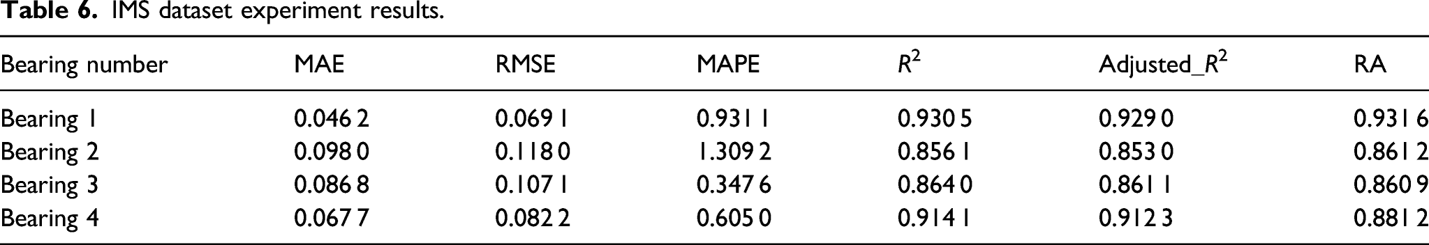
IMS dataset experiment results.

Bearing number	MAE	RMSE	MAPE	R ²	Adjusted_R²	RA
Bearing 1	0.046 2	0.069 1	0.931 1	0.930 5	0.929 0	0.931 6
Bearing 2	0.098 0	0.118 0	1.309 2	0.856 1	0.853 0	0.861 2
Bearing 3	0.086 8	0.107 1	0.347 6	0.864 0	0.861 1	0.860 9
Bearing 4	0.067 7	0.082 2	0.605 0	0.914 1	0.912 3	0.881 2

Table 7.

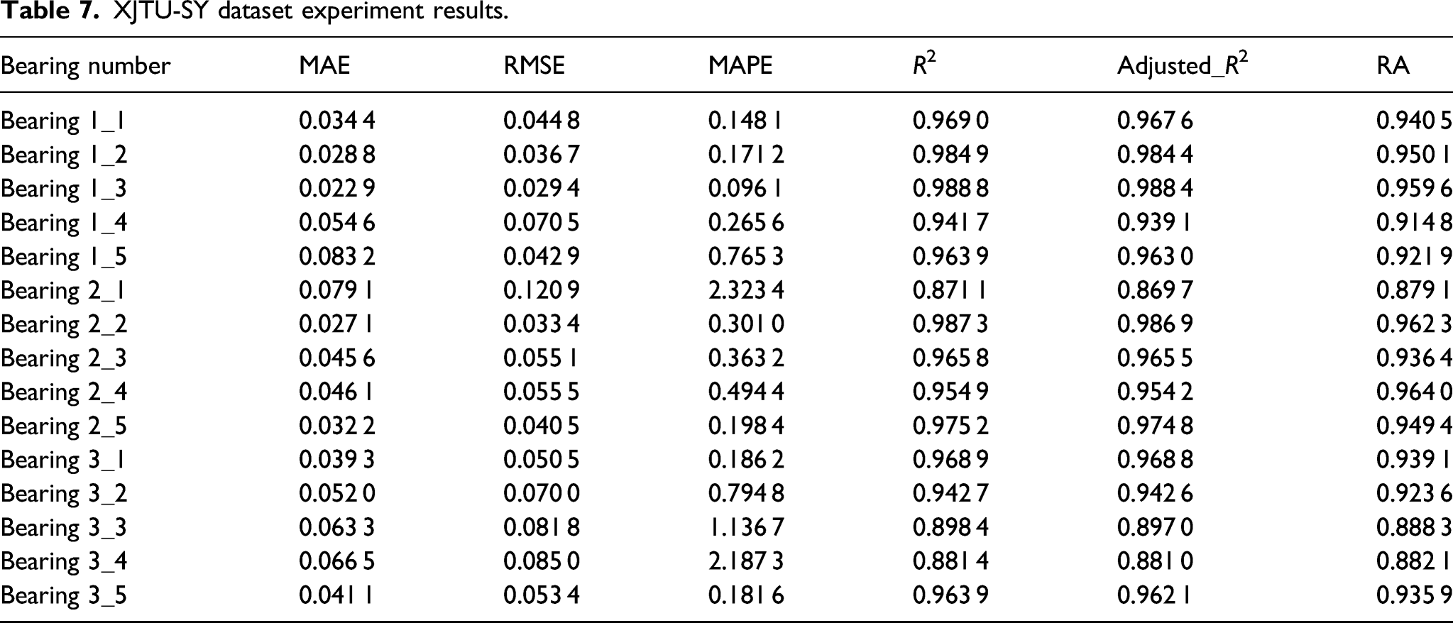
XJTU-SY dataset experiment results.

Bearing number	MAE	RMSE	MAPE	R ²	Adjusted_R²	RA
Bearing 1_1	0.034 4	0.044 8	0.148 1	0.969 0	0.967 6	0.940 5
Bearing 1_2	0.028 8	0.036 7	0.171 2	0.984 9	0.984 4	0.950 1
Bearing 1_3	0.022 9	0.029 4	0.096 1	0.988 8	0.988 4	0.959 6
Bearing 1_4	0.054 6	0.070 5	0.265 6	0.941 7	0.939 1	0.914 8
Bearing 1_5	0.083 2	0.042 9	0.765 3	0.963 9	0.963 0	0.921 9
Bearing 2_1	0.079 1	0.120 9	2.323 4	0.871 1	0.869 7	0.879 1
Bearing 2_2	0.027 1	0.033 4	0.301 0	0.987 3	0.986 9	0.962 3
Bearing 2_3	0.045 6	0.055 1	0.363 2	0.965 8	0.965 5	0.936 4
Bearing 2_4	0.046 1	0.055 5	0.494 4	0.954 9	0.954 2	0.964 0
Bearing 2_5	0.032 2	0.040 5	0.198 4	0.975 2	0.974 8	0.949 4
Bearing 3_1	0.039 3	0.050 5	0.186 2	0.968 9	0.968 8	0.939 1
Bearing 3_2	0.052 0	0.070 0	0.794 8	0.942 7	0.942 6	0.923 6
Bearing 3_3	0.063 3	0.081 8	1.136 7	0.898 4	0.897 0	0.888 3
Bearing 3_4	0.066 5	0.085 0	2.187 3	0.881 4	0.881 0	0.882 1
Bearing 3_5	0.041 1	0.053 4	0.181 6	0.963 9	0.962 1	0.935 9

1. PHM dataset experiment results

For the PHM 2012 data set test, it can be seen that the prediction effect under the three working conditions is still relatively good, and the trend of the remaining life of the bearing can be predicted relatively well. The load of the first working condition is 4 kN, which is relatively low in the comparative experimental load, so the running time of the bearing is relatively long. The corresponding acquisition time is relatively long, and the collected training data is relatively long, so the training effect of the model is better. The load of the second working condition is 4.2 kN. As the load increases, the rotation speed decreases accordingly. The running time of the bearing decreases correspondingly, and the collected data also decreases, but the CNN model after training can still predict it well. The load of the third working condition is 5 kN. In the same period experiment, the load of the third working condition is the largest, the running time of the corresponding bearing is shorter, and the collected data is less. The number of CNN model training samples is greatly reduced, and the error of the corresponding model is also relatively large. However, due to the use of stratified sampling training ideas, the prediction effect of the model is still relatively good, and the RUL of the bearing can still be predicted relatively well (Figure 10 and 11).

Figure 10.

Prediction results of three types of bearings. (a) prognostics and health management bearing 1_1 predicted result, (b) prognostics and health management bearing 1_3 predicted result (c) Intelligent Maintenance System bearing one predicted result, (d) Intelligent Maintenance System bearing four predicted result, (e) XJTU-SY bearing 1_1 predicted result, (f) XJTU-SY bearing 3_1 predicted result.

Figure 11.

Comparative evaluation indicators of three types of bearings. (a) prognostics and health management bearing 1_1 comparative evaluation indicators, (b) prognostics and health management bearing 1_3 comparative evaluation indicators, (c) Intelligent Maintenance System bearing 1 comparative evaluation indicators, (d) Intelligent Maintenance System bearing 4 comparative evaluation indicators, (e) XJTU-SY bearing 1_1 comparative evaluation indicators, (f) XJTU-SY bearing 3_1 comparative evaluation indicators.

2. IMS dataset experiment results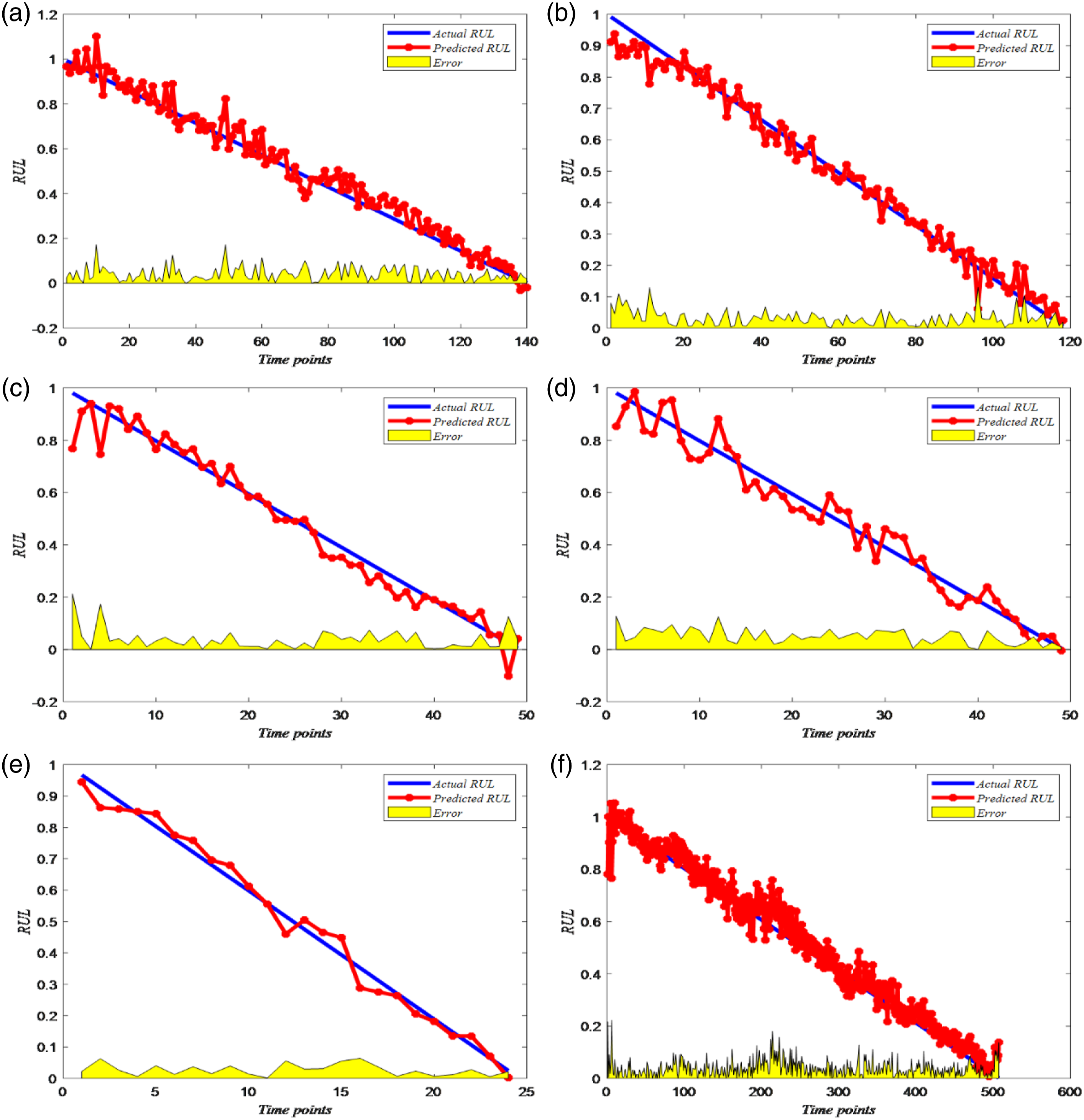

For the IMS dataset, the vibration acceleration signals of the four rolling bearings in the second set of experiments of the database selected in this paper are used as the signal data of the full life of the bearing. The fault type is manifested as an outer ring fault with a total duration of 164 h. It has a radial load of 26.69 kN and is installed on the same shaft. It maintains a constant speed of 2000 r/min. It can be seen that the test results of the IMS data set show that the effects of bearing 1, bearing 2 and bearing 4 are better. The result of bearing 3 is slightly worse, but the remaining life of the bearing can still be predicted comparatively.

3. XJTU-SY dataset experiment results

For the XJTU-SY dataset, the radial load of the five bearings in working condition one is 12 kN, which is the largest in the same period of experiment, and the corresponding speed is the lowest. Therefore, the running time of the bearing is also relatively short. The data is relatively small, but the prediction effect of our proposed method is still relatively good. The radial load of working condition 2 is 11 kN, and the speed increases as the radial load decreases. Therefore, the amount of collected data is also relatively large, and the prediction results of the model are also relatively good. The radial load of working condition 3 is 10 kN, the maximum speed is 2400 r/min, and the collected data is also the most. Therefore, the trained CNN model is better, and the final prediction result is also better.

Evaluation indicators

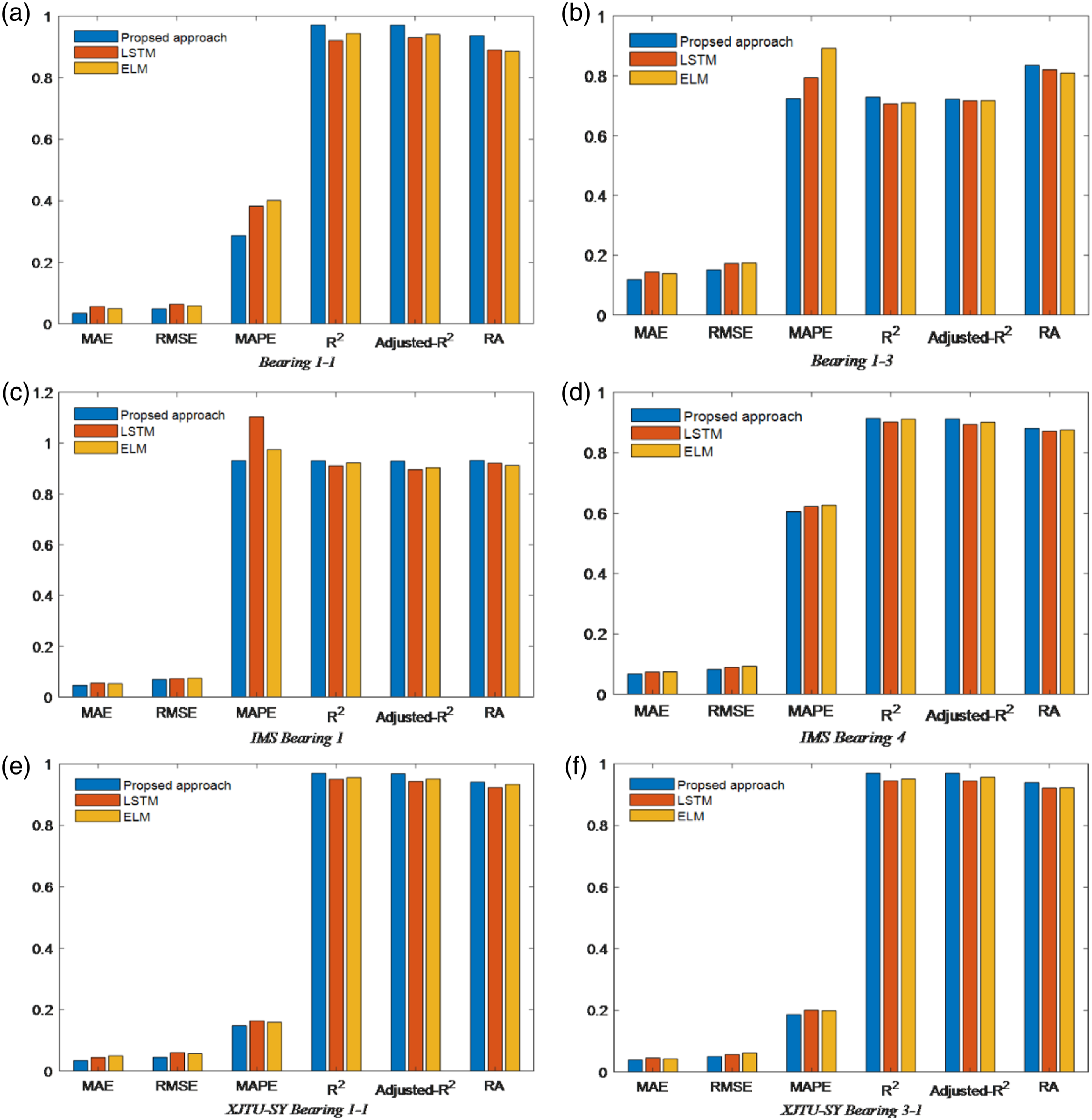
As a comparison, LSTM and ELM are selected for comparative experiments. Among them, the number of nerve cells in each hidden layer of LSTM is 200, and the number of hidden layers is 5. The weights of the ELM input layer and the offset of the hidden layer are randomly selected numbers. The results show that the experimental results in this article are due to the above two methods. Two bearings are selected for each data set for comparison experiment.

In the two datasets selected for PHM, the MAE of Bearing 1_1 is 0.034 2, RMSE is 0.049 0, MAPE is 0.287 0, R² is 0.971 5, Adjusted_R² is 0.971 2, and RA is 0.937 1. Among them, MAE, RMSE, and MAPE are all smaller than the prediction effects obtained by ELM and LSTM, and R², Adjusted_R², and RA are all higher than the prediction accuracy of the above two models, indicating that the model proposed in this paper is superior to the above two models.

In the two datasets selected for IMS, the MAE of Bearing 1 is 0.046 2, RMSE is 0.069 1, MAPE is 0.931 1, R² is 0.930 5, Adjusted_R² is 0.929 0, and RA is 0.931 6. Among them, MAE, RMSE, and MAPE are all smaller than the prediction effects obtained by ELM and LSTM, and R², Adjusted_R², and RA are all higher than the prediction accuracy of the above two models.

However, the MAPE of the IMS dataset is generally a little larger, mainly because the sampling frequency of the IMS is relatively high, and the number of sampling data points is relatively large. MAPE is a cumulative sum index, so compared to other datasets, the MAPE result of the IMS dataset is a bit larger.

In the two datasets selected for XJTU-SY, the MAE of Bearing 1_1 is 0.034 4, RMSE is 0.044 8, MAPE is 0.148 1, R² is 0.969 0, Adjusted_R² is 0.967 6, and RA is 0.940 5. Among them, MAE, RMSE, and MAPE are all smaller than the prediction effects obtained by ELM and LSTM, and R², Adjusted_R², and RA are all higher than the prediction accuracy of the above two models, indicating that the model proposed in our paper is superior to the above two models.

Among the three RUL prediction methods, it is obvious that proposed method has the smallest error and best fitting effect compared with other methods.

Conclusion

In this paper, a new RUL prediction method based on fractal dimension and convolution neural network is proposed. First, this method introduces fractal dimension into the characterization of rolling bearing fault characteristics, and combines time domain, frequency domain, wavelet packet domain and entropy domain to construct multi-dimensional fusion features, which can reveal the degradation state of rolling bearings more comprehensively. Secondly, the percentage of remaining life of the bearing is used as a tracking metric label, and training samples and test samples are divided based on the idea of hierarchical data sampling. Finally, a 6-layer one-dimensional convolutional neural network is constructed to fit the hidden non-linear mapping relationship between the multi-dimensional fusion features and the percentage of remaining life, so as to perform RUL prediction. Experimental verification is carried out on three common full-life rolling bearing data sets. The results show that compared with LSTM and ELM, the prediction effect of rolling bearing remaining life based on fractal dimension and CNN is improved.

In the future, we will consider the remaining life prediction of different types of bearings, and combine the currently popular methods of constructing health indexes(HI) to predict RUL. Moreover, some methods of adaptively extracting and extracting features should also be applicable. Other potential degradation indicators will be attempted to be combined with the CNN model for even higher health prognosis accuracy.

Footnotes

Declaration of conflicting interests

The author(s) declared no potential conflicts of interest with respect to the research, authorship, and/or publication of this article.

Funding

The author(s) disclosed receipt of the following financial support for the research, authorship, and/or publication of this article: This work was supported in part by the National Natural Science Foundation of China under Grant 61671338 and Grant 51877161.

ORCID iDs

Guorong Ding

Wenbo Wang

References

Wang

Kang

, et al. Method of Predicting Remaining Useful Life of Rolling Bearing Combining CNN and LSTM. J Vibration, Measurement Diagn, 2021.

Pan

Hong

Chen

, et al. Performance degradation assessment of a wind turbine gearbox based on multi-sensor data fusion. Mechanism Machine Theor 2019; 137: 509–526.

Dai

Chen

Tao

. Research on PHM model of point machine based on dynamic PSO to optimize HSMM. Railway Stand Des 2018; 62(09): 174–178.

Jun

Gao

Huang

, et al. Prediction of fatigue life of turbine blades based on QAR data[J]. J Syst Simulation 2019; 31(06): 1165–1171.

Zeng

Yang

Zou

, et al. Bearing life prediction method based on parallel multi-channel convolutional long and short-term memory network. China Mech Eng 2020; 31(20): 2454–2462+2471.

Xia

Song

Zheng

, et al. An ensemble framework based on convolutional bi-directional LSTM with multiple time windows for remaining useful life estimation. Comput Industry 2020; 115: 103182.

Aye

Heyns

. An integrated Gaussian process regression for prediction of remaining useful life of slow speed bearings based on acoustic emission. Mech Syst Signal Process 2017; 84: 485–498.

Loutas

Roulias

Georgoulas

. Remaining useful life estimation in rolling bearings utilizing data-driven probabilistic E-support vectors regression. IEEE Trans Reliability 2013; 62(4): 821–832.

Zhang

. Bearing life prediction of subway fan based on EMD noise reduction and LSTM network. Fan Technol 2020; 62(3): 77–82.

10.

Lecun

Bengio

Hinton

. Deep learning. Nature 2015; 521(7553): 436–444.

11.

Jun

Nan

Weiwen

. Estimation of bearing remaining useful life based on multiscale convolutional neural network. IEEE Transactions on Industrial Electronics 2018; 66: 1–11.

12.

Kang

Zhou

Wang

, et al. Rolling bearing RUL prediction method based on improved SAE and bidirectional LSTM. Acta Automatica Sinica 2020; 11: 1–11.

13.

Tian

. An artificial neural network method for remaining useful life prediction of equipment subject to condition monitoring. J Intell Manufacturing 2012; 23: 227–237.

14.

Sun

Zhang

. Research on bearing life prediction based on support vector machine and its application. J Phys Conf Ser 2011; 305(1): 012028.

15.

Ren

Cui

Sun

, et al. Sun Yaqiang, etcMulti-bearing remaining useful life collaborative prediction: A deep learning approach. J Manufacturing Syst 2017; 43: 248–256.

16.

Cao

. Bearing remaining service life prediction based on parallel CNN-SE-Bi-LSTM. Computer Application Research 2021; 99: 1–6. DOI: 10.19734/j.issn.1001-3695.2020.08.0224.

. Bearing remaining life prediction based on one-dimensional convolutional neural network. Manufacturing Automation 2020; 42(03): 10–13.

, et al. A remaining useful life prediction method bearing based deep neural networks. Meas 2021; 172: 108878.

19.

Yoo