Anisotropy magnetoresistance differential probe for characterization of sub-millimeter surface defects on galvanized steel plate

Abstract

Defects such as cracks can cause dangerous damage to the metal structure and may lead to structural collapses. Cracks can exist in various shapes and sizes where they can start to develop from small scale lower than 1 mm and spread to contribute to the complete fracture of components. Hence, early discovery and monitoring of any cracks in their early stage are crucial to prevent any sudden fatal accidents in the future. This work presents the study and detailed analysis of an ECT probe’s development based on AMR sensors to identify sub-millimeter surface cracks in galvanized steel plates. The probe consists of an excitation coil that induces an eddy current in sample plates and two AMR sensors that detect the differential eddy current-induced magnetic response. A phase-sensitive detection technique with a lock-in amplifier is used to evaluate the magnetic field distribution detected by the AMR sensors. The measured magnetic responses are classified to the depth, width, length, and complex shapes of artificial slits, and the probe is used to perform line scans and 2-D map scans above the slits’ positions. The probe was able to characterize slits with a depth and width as low as 210 and 50 µm, respectively, by using an excitation current of 4 mA at 1 kHz. The slit orientations that were perpendicular to the differential direction of the AMR sensors were clearly visualized, with their estimated lengths showed a good correlation with the physical slit lengths. In the future, the developed system can be expected to help towards the development of a more sophisticated crack detection system where real-time inspections can be realized and applied in various fields.

Introduction

Characterization of magnetic field distributions induced by defects is a promising technique for NDT of steel materials since they are non-contact, rapid, and safe. This magnetic field characterization procedure also possesses an advantage in which it can be compacted easily since its system configuration is simple. Methods that use this technique include the eddy current testing (ECT) method, where in NDT, ECT is broadly used for the evaluation of conductive components such as metallic plates.^1,2

Commonly, the causes of failure towards the steel structures are because fatigue, machining tears, and corrosion, where these defects can cause an accident and harmful to the structures. ² Surface and subsurface cracks are one of the defects that must be monitored in order to avoid accidents that can lead to severe injury or death. ³ Moreover, the structural safety of samples under test must also be ensured where a continuous inspection without causing any deterioration of them is needed.

Recent reviews state that the magnetic field characterization method is one of the auspicious methods when dealing with steel structure. Conventionally, a coil is used as a medium to detect the secondary magnetic field produced by the repeated eddy currents in most ECT probes. However, due to the frequency-dependent behavior of the inductive coil, it is conveniently used for surface defect detection only. ⁴ In acoil-based probe, a high frequency of the excitation field is used to allow for highly sensitive detection of failures in a metal specimen. According to the previous reports, the adequate frequency to produce an eddy current for surface crack detection in a steel material is between 1 and 2 MHz, based on penetration depth δ expression.^5,6 Moreover, the induction coil used to detect the eddy current in the probe is also hard to be compacted since its sensitivity depends on its geometrical factors. Since the coil is sensitive at high frequency, it requires a high number of conductive windings to detect a magnetic field, which can lead to an increase in the probe size. Even though this technique is promising, but to detect a small defect or crack in material, especially inside the metal or backside of the metal, a low-frequency and high-spatial-resolution sensor is required.

There are few techniques that involve the basic principle of eddy current, ⁷ and those techniques depend on identifying the eddy currents created by an applied magnetic field and supervise the changes of the eddy current flow ⁸ so that the presence of the defect can be detected. Moreover, compared to other methods, the eddy current measurement approach is better because the investigation can be done with the tested material without any contacts. ⁹ These techniques can be labeled as Eddy Current Testing (ECT) and Pulsed Eddy Current (PCT) techniques.^10,11 This method was increasingly developed significantly in the aircraft and nuclear ¹² industries since the 1950s.

ECT is able to detect a crack in various conductive materials, either ferromagnetic or non-ferromagnetic. However, the ECT method is rarely applied to ferromagnetic materials because the detected magnetic field consists of both information of the eddy current and strong magnetization signal. ¹³ Since the magnetization signal causes trouble in finding defects on the sample, therefore, a measurement technique is needed to lessen the magnetization signal below the eddy current’s signal to avoid a detection error and other magnetic noises. Because of that, the ECT method is frequently operated on non-ferromagnetic material such as aluminium because its magnetization signal is small; thus, easier to detect eddy current signal. ¹⁴ The galvanized carbon steel plate, on the other hand, has been widely used in industries due to its excellent rust resistance. However, applying the eddy current measurement technique for defect detection in the galvanized steel plate can be difficult. ¹⁵ This is due to the fact that the galvanized steel plate is a ferromagnetic material where the magnetic response from the plate contains both eddy current and strong magnetization signals.

Cracks can exist in various shapes and sizes where the crack can develop from a small scale lower than 1 mm. The size of cracks can spread and contribute to the complete fracture of components. Hence, the discovery of any cracks in their early stage will prevent any sudden fatal accidents in the future. In order to detect small sizes of cracks, a highly sensitive probe is required from the low-frequency region. ¹⁶ Thus, the ordinary probe using coils to detect eddy current signal has been replaced by magneto-resistive (MR) magnetometers. ¹⁷ MR magnetometers are promising detector tools since they are highly sensitive, able to detect small signals produced by tiny flaws, and can be compacted in a small package.

A low-frequency ECT technique is used in this study to allow a deeper detection of flaws since the skin depth effect governs the induced eddy currents. AMR sensors (Honeywell HMC1001) are used to fabricate this NDT system so that it can achieve a highly sensitive measurement. The AMR sensor is advantageous over the coil-based magnetic sensor owing to its sensitivity from DC to a few kHz. To construct the ECT system, many magnetometers have been used, such as inductive coil, ¹⁸ hall sensor, ¹⁹ Tunnelling Magnetoresistance (TMR) sensor,^13,20 anisotropic magnetoresistance (AMR) sensor,^21,22 fluxgate and superconducting quantum interference device (SQUID). ²² A study shows that SQUID has the lowest noise compare to other sensors. ⁵ However, SQUID may not be convenient to use since performing NDT using SQUID needs liquid nitrogen or liquid helium for the cooling. A comparison of the noise spectral densities in the commercial magnetic sensors presented in Tumanski ¹⁸ and He ²³ showed that the AMR sensor was among the sensors that had the low magnetic field noise in the range of hundreds pT/√Hz.

Methodology

Detection technique

The main objective of the ECT probe in this research is to detect micro-cracks; hence a small ECT probe is advantageous for measuring a small or complex shape of defects.^13,24 Since the AMR sensor is relatively small in size, the ECT probe size can be further compacted compared to the use of coil while also addressing the magnetic noise issue in conductive materials. Furthermore, the output signal from the ECT probe can be analyzed using the signal vector method and lock-in amplifier. In the lock-in detection, a reference signal for the phase-sensitive detection is required. The reference signal is used to measure the phase delay of magnetic response induced by the eddy current. Due to this, it can cause inaccurate detection of a crack in the material if the phase signal is incorrect. By this technique, the dependency of distribution of the magnetic properties of the metal plates can be thought to be reduced by correctly selecting the reference signal. To further reduce the background signals, the differential sensor technique can be used. However, the disadvantage of using this method is that the data of the absolute reading and the local data of the properties of magnetic and physical properties of the sample are lost because of the differential technique. However, this may not be an issue if identifying the change of eddy currents due to defects in materials is the main interest in an eddy current measurement.

During line scanning of the cracks, the probe runs in the path of the x-axis. This probe works to detect eddy current change when the eddy current stumbles upon defects. The detected signal will change by following the flow of the current. For an explanation, a current that is in y-direction will produce two magnetic fields in the x- and z- directions, B_x and B_z, respectively. If the crack in the material is in the y-direction, this will block and redirect the current to the y-direction. According to Maxwell’s equations, the y-directed current can be determined by measuring the magnetic fields that are perpendicular to the current direction. If eddy current is assumed to accumulate on a surface, this results in a non-volumetric current where eddy current can be considered in x- and y-directions only, where;

$$\begin{array}{c}{J}_x=\frac{1}{{\mu }_0}\frac{d}{\mathrm{dy}}\left[B_z{e}^{(-z\frac{\sqrt{\omega \mu \sigma }}{2})}{e}^{(-\mathrm{jz}\frac{\sqrt{\omega \mu \sigma }}{2})}\right]\hfill \\ J_y=\frac{1}{{\mu }_0}\frac{d}{\mathrm{dx}}\left[B_z{e}^{(-z\frac{\sqrt{\omega \mu \sigma }}{2})}{e}^{(-\mathrm{jz}\frac{\sqrt{\omega \mu \sigma }}{2})}\right].\hfill \end{array}$$

(1)

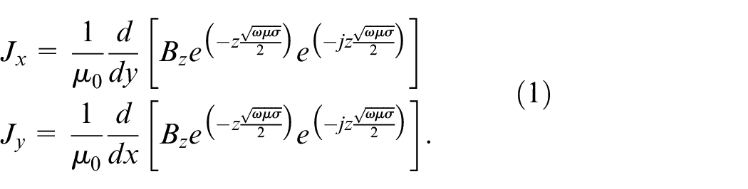
From the above equation, both J_x and J_y contain the same B_z element. From here, it can be concluded that it is convenient to have a measurement using one sensitive axis only. In this case, the measurement of magnetic field response in the z-axis is chosen to develop the probe. By using information from B_z, the current density J_x and J_y can be estimated since B_z contains both information of J_x and J_y. However, to get a precise estimation of the current, the magnetic field response must be measured in three directional axes, that is, B_x, B_y, and B_z. On the other hand, this current vector can be simply estimated by the Hosaka-Cohen transformation. ²⁴

To verify the distribution of magnetic field produced by a line current, a simulation is performed. Figure 1 below shows the simulation of magnetic field distribution produced by a line current having the x- and y- directions.

Figure 1.

Magnetic field distribution produced by a line current in the x- and y- direction: (a) Bx, (b) By, (c) Bz, (d) differential of magnetic distribution with respect to the position of line current in the x-direction, (e) differential of magnetic distribution with respect to the position of line current in the y-direction and (f) arrow map of the reconstructed current dipole using the Hosaka-Cohen transformation.

In the simulation, the current dipole is created in the x- and y - directions. From Figure 1, the current dipole is shown as the black line. According to Bio-Savart’s law, the current dipole will create a magnetic field where B_x, B_y, and B_z is the components of the magnetic field. From Figure 1(a) and (b), it can be shown that each direction of the current dipole has its own magnetic field distribution characteristics. In contrast, Figure 1(c) shows that the magnetic field distribution B_z covers all areas for both x- and y - directions. Therefore, it can be concluded that it is more convenient to take B_z into consideration during the probe development as it can cover the different directions of the current.

Figure 1 (d) and (e) show the differential of magnetic distribution B_z with respect to the current dipole. Similar to Figure 1 (a) and (b), each of the current dipoles has its own magnetic distribution characteristics. The differential signal of the B_z -component is equivalent to a gradient of ΔB_z/Δx ≈∂ B_z/∂ x or ΔB_z/Δy ≈∂ B_z/∂ y. Figure 1(f) shows the arrow map where the a_x and a_y are unit vectors. From Figure 1(f), it shows clearly that the location and direction of current in every direction can be estimated by the vector a , which can be determined by measuring ∂ B_z/∂ x and ∂ B_z/∂ y.

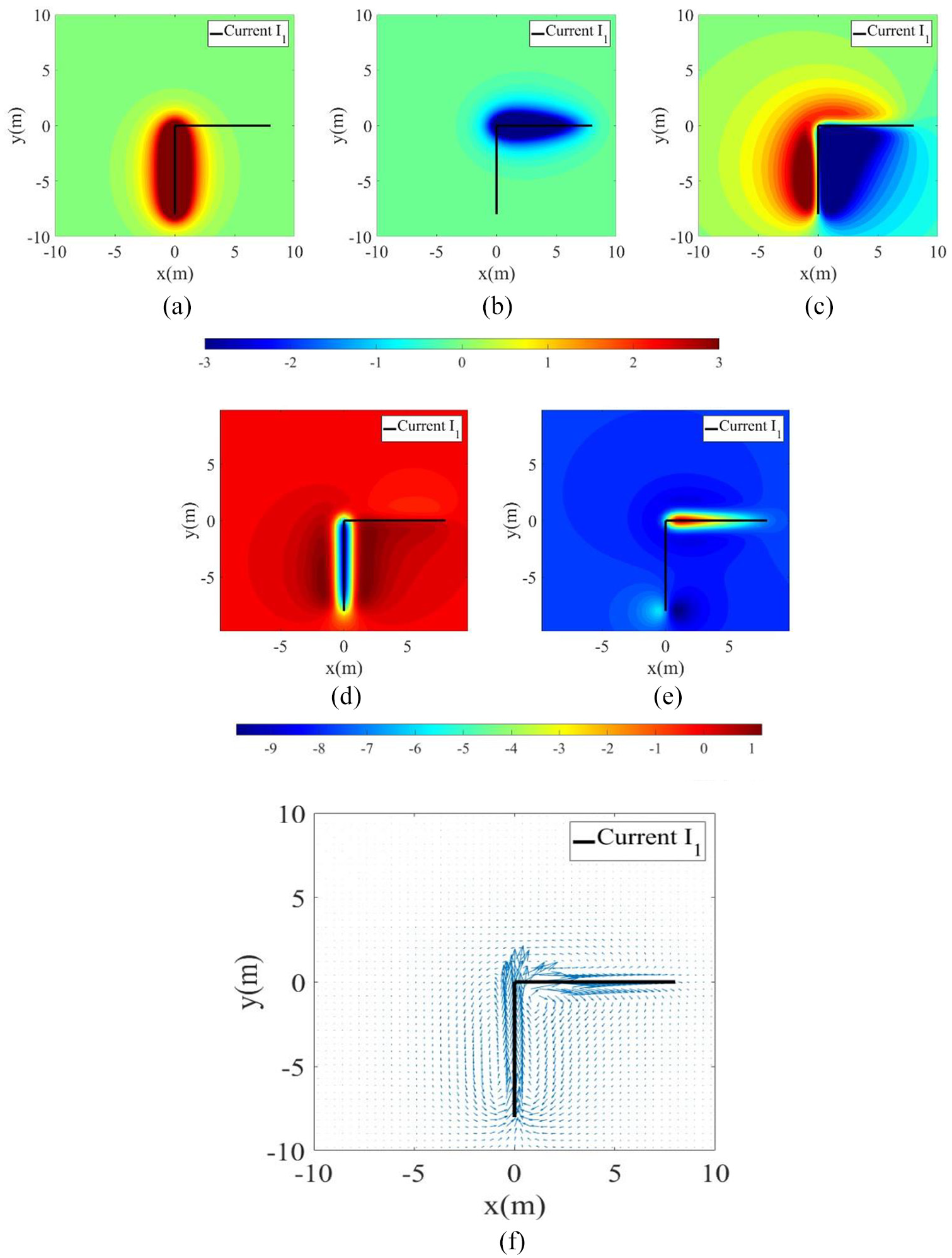
During the defect detection process, an AC magnetic field will be applied to a conductive sample. The primary magnetic field will penetrate into the conductive sample, and a repeated eddy current is induced subsequently within the sample volume. Then, the eddy currents will result in the generation of the secondary magnetic field. In this study, two AMR sensors are used to sense this secondary magnetic field, and their sensitive axis is placed perpendicular to the surface of the sample, that is, the z-direction. However, in a ferromagnetic steel component, besides the eddy current signal, a magnetization signal due to the material permeability is also generated. The combination of both signals detected can be represented by a vector with a phase lag shown in in Figure 2(a). The detected magnetic response from a magnetic sensor (sensor 1) after the phase lag correction can be denoted by S₁ as shown in Figure 2(b), where it contains a large magnetization signal S_mag,1 due to the magnetization curve M-H characteristic^25,26 and small eddy current-induced signal S_eddy,1. Here, a phase-sensitive technique using the lock-in amplifier is used to separate S₁ into two components where the real and imaginary parts correspond to S_mag and S_eddy, respectively. Moreover, it also should be noted that the applied magnetic field may couple and be detected by the magnetic sensor due to the stray flux.

Figure 2.

(a) The induced magnetic response B_induce with a Phase lag α at the plate surface, (b) the differential vector of the measured magnetic signals from two AMR sensors, containing eddy current contributed signal S_eddy and magnetization signal S_mag and (c) illustration of the working principle of ECT.

When there is an anomaly presents in the sample, the density and direction of the eddy current distribution S_eddy,1 will be changed due to the existence of the anomaly. At that point, by using S₁ as the reference signal, the intensity of the differential vector S _eddy,1 – S _eddy,2 is calculated. Since S_mag,1 is reduced by means of the difference between the sensors, the phase difference of the small eddy current can be identified between S₁ and S₂. It should be emphasized that the baseline of the sensor and the size of the excitation coil have a considerable effect on S_mag,1 since the magnetic properties’ distribution may exist over the sample.

Sensor baseline and lift-off

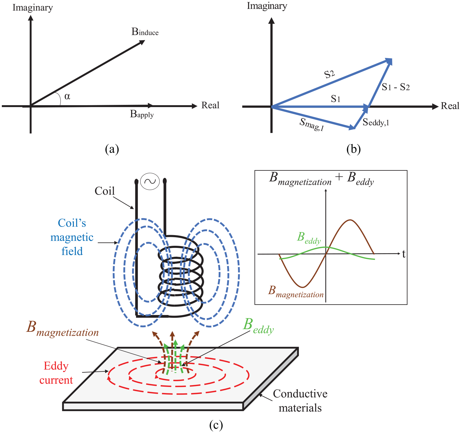
Figure 3 shows the graph of simulated magnetic response from a line current of 1 mA with different baselines from 1 to 9 mm. It shows that the smaller the baseline, the clearer and more accurate the location of the current can be detected.

Figure 3.

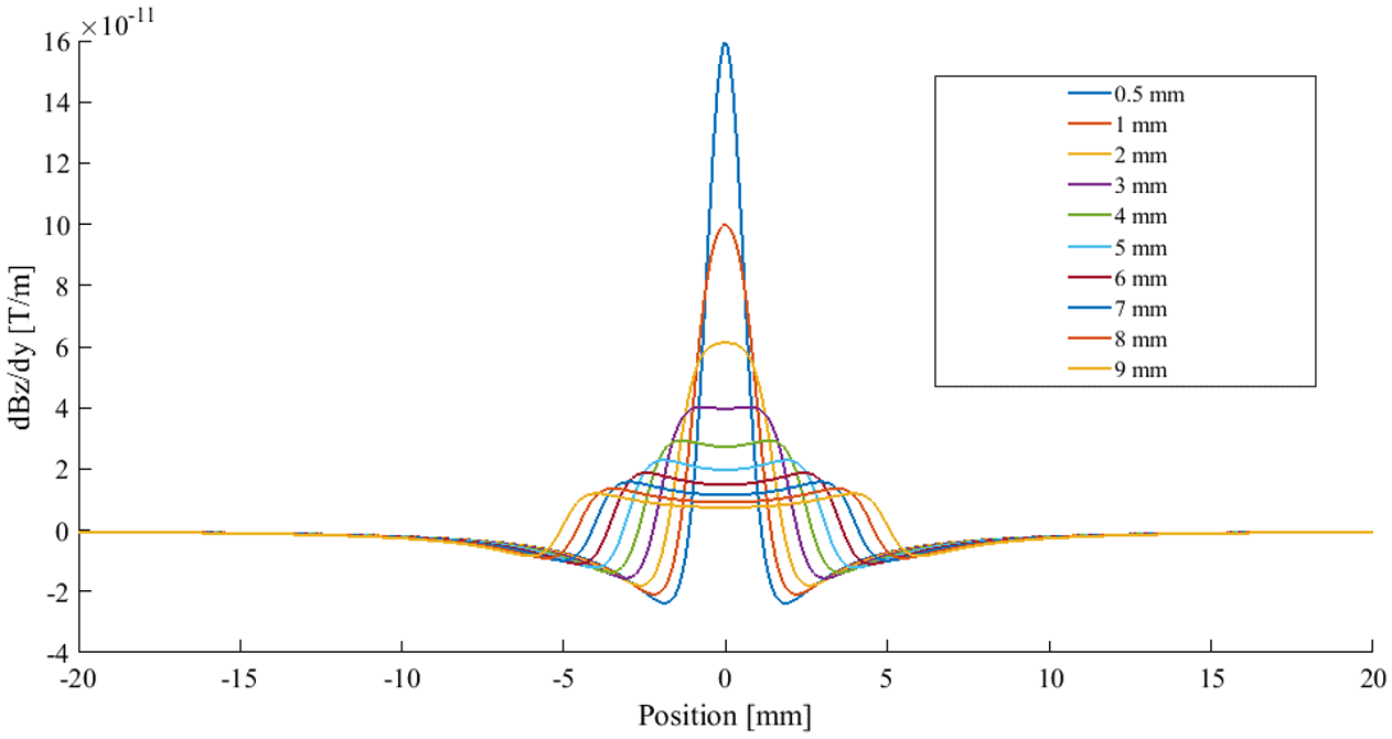
Magnetic response with different baseline.

Eddy current NDT has always been related to the lift-off problem. The amount of lift-off is strongly affected in the ECT, where it can be defined as the separation of the sensors and the conducting material surface. Lift-off plays an important role in affecting the signal-to-noise ratio (SNR) of the detected magnetic response, where it can cause adverse effects and limit the detection of eddy currents if the lift-off is enormous. Figure 4 shows the simulated effect of lift-off and baseline from 1 to 9 mm to the signal attenuation of the differential probe. Figure 4 was plotted by measuring the characteristic between peaks and troughs, as shown in Figure 3, due to the line current. This simulation also implied that the skin effect to the magnetic field distribution could be related by investigating the magnetic field distribution at different lift-off, that is, the difference of depth level of the eddy current was equivalent to the different level of lift-off. Moreover, the signal attenuation was more affected by the lift-off compared to the baseline; however, it could be expected that the accuracy of the eddy current localization would be decreased.

Figure 4.

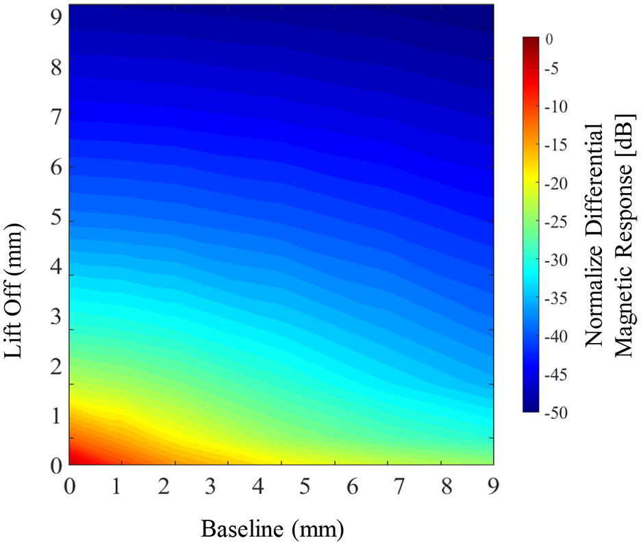
Magnetic response distribution of lift off effect.

Overall system development

The developed ECT system consists of few elements such as an ECT probe, current source for the excitation coil, lock-in amplifier (LI 5640, NF Corporation), sensor circuits, XY stage, and computer for data acquisition and evaluation. The AMR sensors will detect a secondary magnetic field that is generated by the eddy current induced by the primary magnetic field. The schematic circuit of the developed ECT probe is shown in Figure 5.

Figure 5.

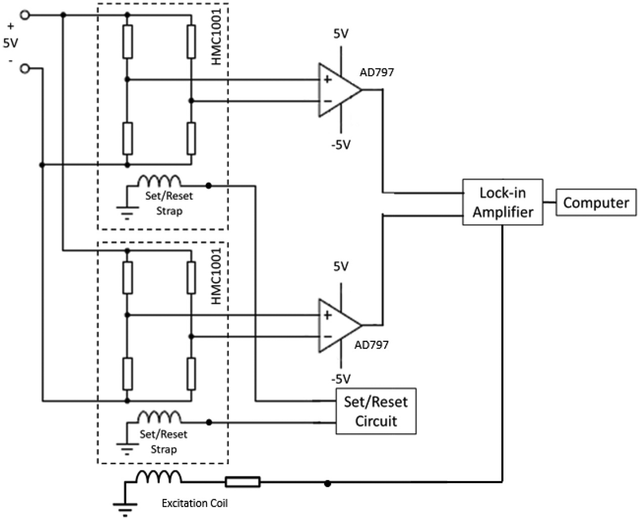
The schematic diagram of the established ECT probe.

ECT probe

In this study, two AMR sensors with each in absolute magnetic field measurement mode are used and configured to form a differential technique. This results in a dual-channel sensor probe. The dual-channel ECT probe consists of double AMR sensors that have been inserted inside an excitation coil. Both AMR sensors are attached together and separated by a 4 mm baseline to detect the differential signal. The baseline of the sensors is set to be 4 mm due to the fabrication limitation for the probe, where each sensor package has a thickness of 1.8 mm.

The AMR HMC1001 sensor (Honeywell) is used in the probe’s development. In this AMR sensor, a Wheatstone bridge is formed by 4 AMR elements, and a supply voltage is used to bias the bridge. ²¹ The resistance of the AMR elements changes and causes the unbalanced voltage between the two midpoints of the bridge branches when a magnetic field is applied. Therefore, an instrumentation amplifier is required so that these two points can be measured accurately and reducing the voltage loading effect.

A high sensitivity detection unit for the AMR bridge outputs is obtained by fabricating a custom-made instrumentation amplifier (INA) by using a 3-operational amplifier (AD797) topology. A Set/ Reset strap in the sensor is used in order to restore the sensitivity of the AMR elements. When a strong magnetic field is applied to the AMR sensor, this will demagnetize the sensor. ²⁶ Once the AMR sensor demagnetizes, the sensitivity of the sensor will be diminished. To regain back the sensitivity, the Set/Reset strap around the AMR elements is used to reset the anisotropy direction. The Set/Reset strap functions when a high current pulse is applied to the Set/Reset strap. This will cause the magnetization of the AMR sensor to be resumed, and the AMR sensor is set to a maximum sensitivity.

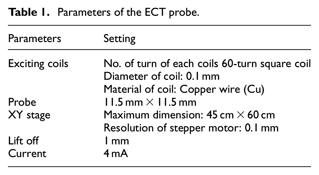
A 60-turn excitation coil is wound around the AMR sensors. This circular coil is selected to produce circular eddy currents instead of linear-direction eddy currents so that the flow of eddy current can be disturbed for vertical and horizontal defects. The amplified magnetic response by the INA will be phase-sensitive detected by the lock-in amplifier and display in a computer. Table 1 gives the parameters of the ECT probe, while the schematic diagram of the developed ECT probe is shown in Figure 6.

Table 1.

Parameters of the ECT probe.

Parameters	Setting
Exciting coils	No. of turn of each coils 60-turn square coil
	Diameter of coil: 0.1 mm
	Material of coil: Copper wire (Cu)
Probe	11.5 mm × 11.5 mm
XY stage	Maximum dimension: 45 cm × 60 cm
	Resolution of stepper motor: 0.1 mm
Lift off	1 mm
Current	4 mA

Figure 6.

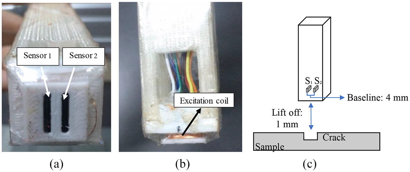
(a) Fabricated sensor probe from the bottom view, (b) photograph of the fabricated excitation coil and (c) arrangement of the sensor probe with respect to the sample.

Sample preparation

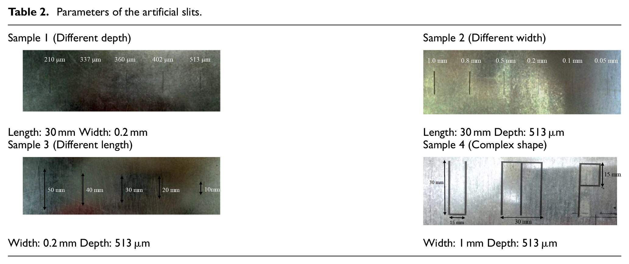
To evaluate the effectiveness of the sensor probe, artificial flaws are laser-engraved on a 2 mm galvanized carbon steel plate. A fiber laser marking machine is used to create the artificial slits by characterizing the magnetic field distributions of the induced eddy currents with regard to the length, width, depth, and different shapes of the slits on ferromagnetic galvanized carbon steel plates at different frequencies of the excitation field. The depth of the slits is characterized using a laser microscope (3D Measuring Laser Microscope OLS5000, Olympus). Table 2 gives the parameters of the defects.

Table 2.

Parameters of the artificial slits.

Sample 1 (Different depth)	Sample 2 (Different width)
Length: 30 mm Width: 0.2 mm	Length: 30 mm Depth: 513 µm
Sample 3 (Different length)	Sample 4 (Complex shape)
Width: 0.2 mm Depth: 513 µm	Width: 1 mm Depth: 513 µm

Results and discussion

Crack detection performance

Line scanning of slits with different depth

The first experiment was conducted by using sample 1 with different depths of the artificial slits as shown in Figure 7, where the depth of the slits was from 200 to 500 micrometer. This section focuses on the characteristic curves of magnetic response dB_z/dx under different frequency conditions. Since the output signal was phase-sensitive detected using a lock-in amplifier, therefore, they had two outputs which were the real dB_z,_real/dx, and imaginary components dB_z,_ima/dx as shown in Figure 8.

Figure 7.

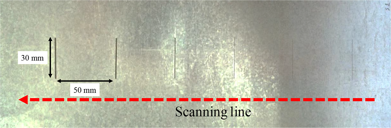
Artificial slits (defect) on a galvanized steel component.

Figure 8.

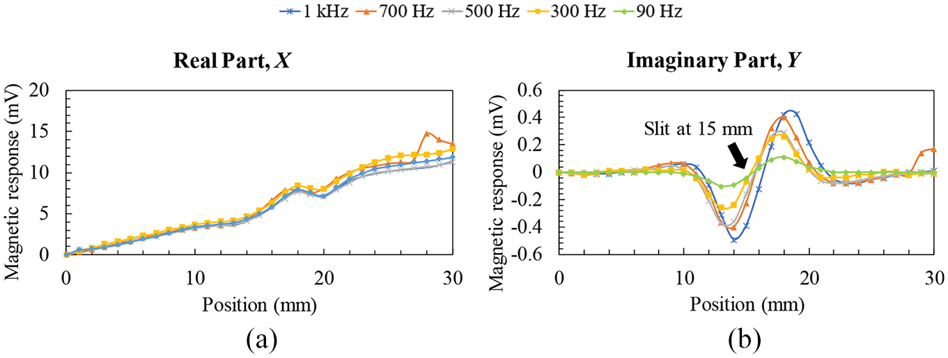
(a) Real components and (b) imaginary components of the line-scanned magnetic field intensities at various frequencies with 513 µm depth of a slit.

However, for the slit detection in the current study, only the imaginary component dB_z,_ima/dx was used. This is due to the fact that the real component dB_z,_real/dx signal did not show any significant changes when being introduced to the slit (Figure 8(a)). This could be thought that the real component dB_z,_real/dx contained strong magnetization signals; hence the weak eddy current signal induced by the slit had no significant effect on the overall real component dB_z,_real/dx signal. On the contrary, the imaginary output signal dB_z,_ima/dx showed a clear difference of the magnetic response at the slit position without any significant signal drift compared to the real component dB_z,_real/dx.

The frequency of the excitation magnetic field was set to be 1 kHz, 700, 500, 300, and 90 Hz during the line scanning experiment of 513-µm depth slit. Compared to other excitation frequencies, a slight change of magnetic response around the slit region was observed for the 90-Hz excitation magnetic field. As the frequency increased, the changes of the magnetic response around the slit area were increased significantly. This was due to most of the eddy currents that had been generated were concentrated to the surface, that is, the skin-depth effect. This resulted in the magnetic AMR sensors detecting the increasing eddy current signals as the frequency was increased.

To signify the difference between the maximum and minimum values of the peaks and trough in the magnetic response waveforms in Figure 8, a delta value of them was calculated and is shown in Figure 9. From Figure 9, the result showed that the signal difference was increased as the slit depth increased. This case was similar to the case when the frequency was increased, where the delta values would increase as well.

Figure 9.

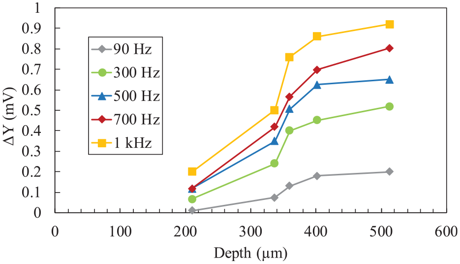
The signal difference between peak and trough of imaginary component waveforms with respect to different depths of slits at different frequencies.

This graph clearly showed that when there was an increase in the excitation frequency, it could be expected that the skin depth would be reduced and resulting in the increment of the detected magnetic response. As the defect detection using the probe was performed on the top surface of the galvanized carbon steel material, therefore, a higher selection of frequency was more suitable to be used where all the eddy current would accumulate on the surface. Nevertheless, a low frequency could also be a preferable choice since it would enable the detection of deeper sub-surface slits.

Magnetic response distribution with different depth

Figure 10 shows the map distributions of the gradient magnetic response dB_z,_ima/dx of the slits with different depths at 1 kHz excitation field. The result displayed a precise intensity change at the slit range, especially for the deepest slit. Moreover, the value of intensity for the deepest slit was higher compared to others, and the value was decreased as the depth of the slits decreased. The gradient of magnetic response showed two intensity peaks where this data agreed with the line scanning data in Figure 8(b).

Figure 10.

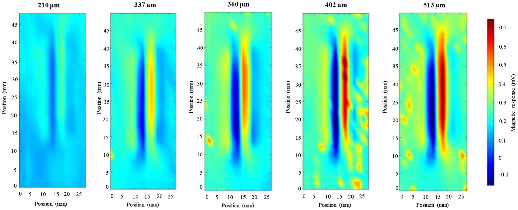
Magnetic map distributions of different slit depths at 1-kHz excitation field.

However, the intensity change still could be seen even though the depth of the slits was only 210 µm. This was due to the high-frequency field where most of the eddy currents accumulated to the surface.

Magnetic response distribution with different width

To investigate the signal change affected by the width of the slits (sample 2), a 2-D scanning was carried out. Figure 11 depicts the 2-D scanned maps of magnetic response distributions measured at a frequency of 1 kHz. The magnetic maps reflected the slit pattern.

Figure 11.

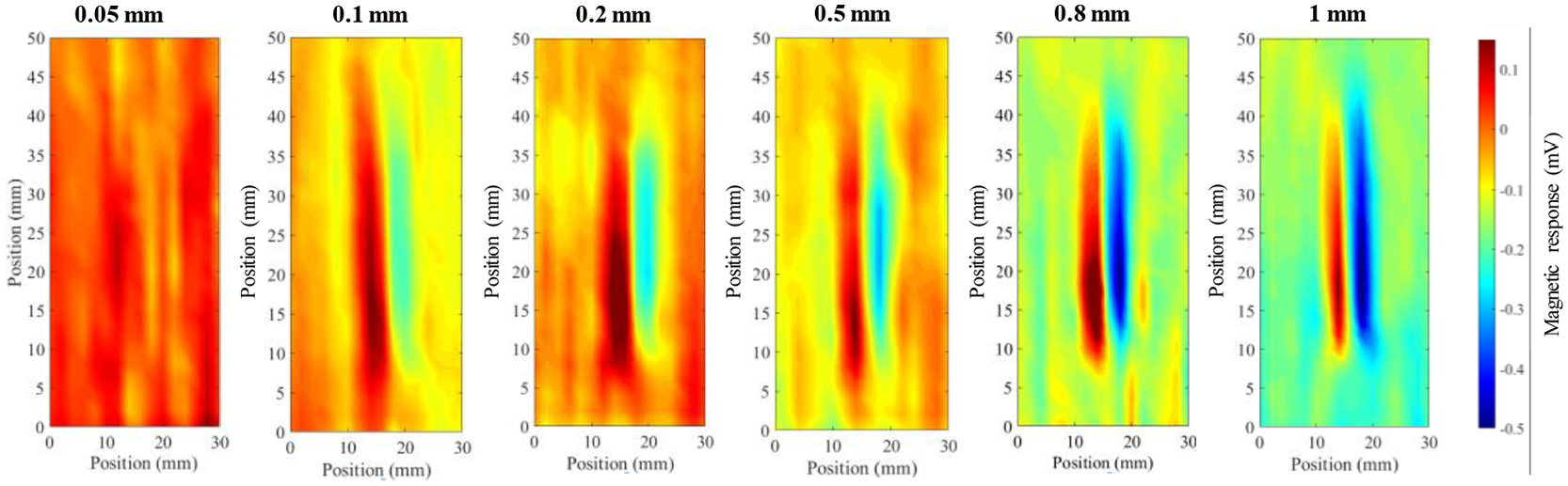
Magnetic map distributions of different slit widths at 1-kHz excitation field.

The shape of the slits could be predicted from the magnetic map obtained through the ECT probe. From Figure 11, the intensity changes were almost invisible for the smallest width. This means that the current limitations of the ECT probe could be 0.5-mm width of slit where if the width of slits was less than 0.05 mm, the signal change would not probably visible. When the slit went wider, the intensity change was getting higher, and this could be seen in the magnetic response distribution map.

Magnetic response distribution with different length

Three parameters could be used to characterize the characteristics of the crack: crack depth, width, and length. Hence, the artificial slits were examined with respect to each of these parameters. In this section, the length of the slits was investigated using sample 3. The magnetic response dependency on the slit length was assessed using the galvanized carbon steel plates with 510 µm deep and 1 mm wide slits at different lengths. Figure 12 shows an apparent length dependence characteristic.

Figure 12.

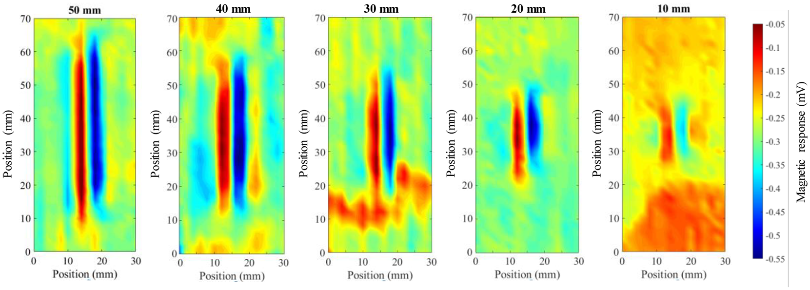
Magnetic map distributions of different slit lengths at 1-kHz excitation field in 2-D.

Since the detection measurement was made for the surface slit, therefore, applying a low frequency would cause a lower signal-to-noise ratio. All the slits could be detected by the probe and clearly be seen in Figure 12 when the measurement was performed at the 1-kHz excitation field. The length of each slit could be clearly seen through the magnetic map distributions in Figure 12.

The magnetic distribution maps showed that the intensity change decreased as the length decreased. From the left side, the real length of the slits was 50 mm, and the magnetic map (Figure 12) showed an almost similar length to the real slits. This was proven when the raw data had been analyzed using the full width at half maximum technique. Figure 13 shows the correlation between the actual size of the slits and the length estimated from the 2D map size of slits using the full width at half maximum technique. From Figure 13, the linear graph shows that the magnetic map of the slits had an almost accurate length with the real length. It could be said that the length of the slit could be accurately estimated from the distribution map of the eddy current.

Figure 13.

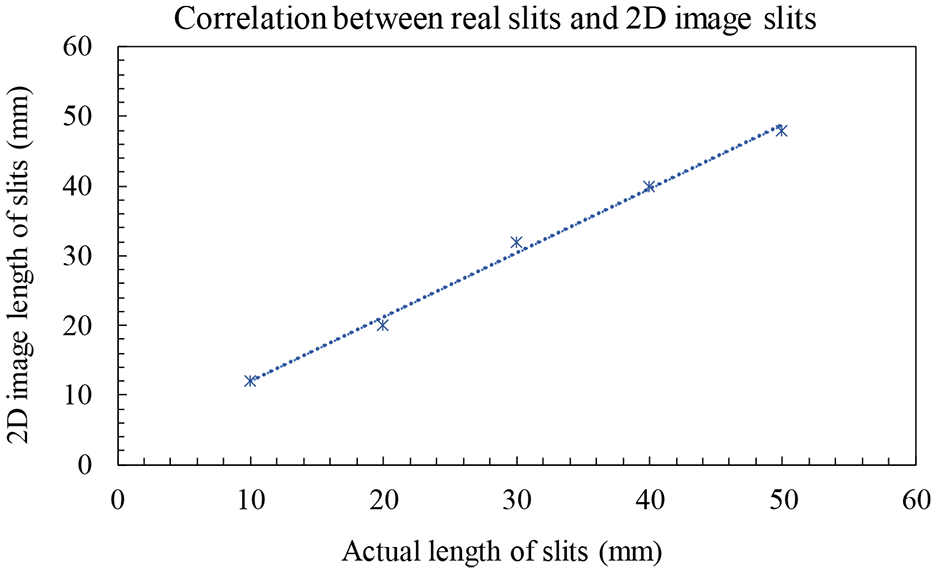
Correlation between the real physical length of slits and the estimated length in the 2D images of magnetic field distributions.

Magnetic response distribution with different shapes

To further evaluate the performance of the ECT probe, a complex shape of slits was prepared where the x- and y-directed slits were combined in one sample. To produce the slits, the laser engraver was used for engraving the sample with letters “U”, “M”, and “P” on the galvanized carbon steel plate with a 2-mm thickness (sample 4). The dimension of the artificial slits was 500 µm in depth and 1 mm in width. The experiment was performed at 1 kHz since it was aimed to detect surface cracks. Figure 14 reveals an obvious intensity change at the location of the slits. However, only the slits in the x-direction cannot be detected by the probe since the probe was set to measure the differential signal of dB_z/dx.

Figure 14.

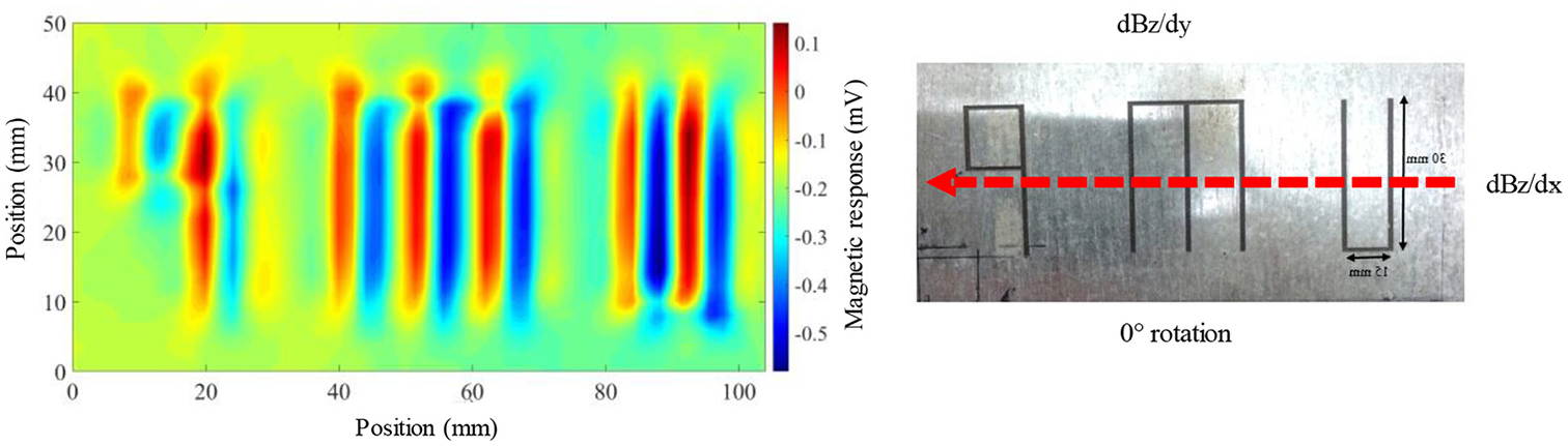
Magnetic map of the steel plate with “UMP” slits using the ECT probe.

From Maxwell’s equations and the Cohen-Hosaka transformation, the gradient magnetic response dB_z/dx was proportional to the dipole current component of J_y where the current density of J_y increased around the slits. This showed that the presence of the slit had directed the eddy current to be parallel with the slits, hence increasing the current density in the y-direction. From Figure 14, the x-directed slits could not be detected, causing the letters to be unclear. The detection sensitivity to perpendicular slits was much higher than that of the parallel slits.

Then, the position of the steel plate was rotated 90° to make sure the probe was sensitive to the x-directed slits. The rotated result is shown in Figure 15, where a clear intensity change at the location of slits especially where x-directed slits are located, was observed.

Figure 15.

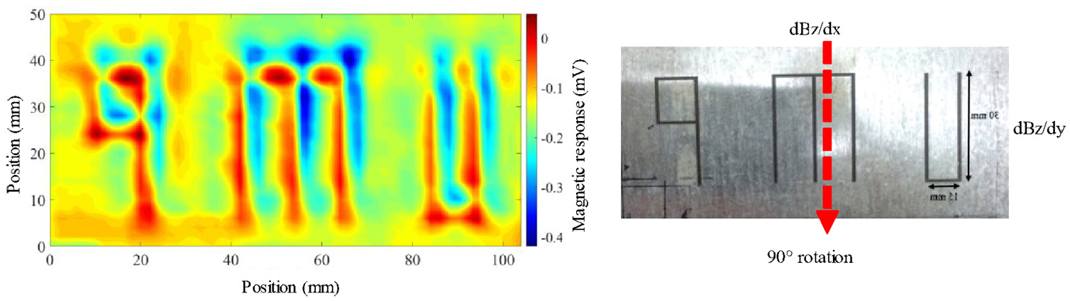
Magnetic map of the steel plate with “UMP” slits using the ECT probe where the letter direction is perpendicular to the ECT probe in 2-D.

Similar to the previous case, according to Maxwell’s equations and the Cohen-Hosaka transformation, the measure of gradient magnetic response dB_z,_ima/dy was proportional to the dipole current of J_x component where the current density of J_x increased around the slits. This proved that the presence of the slits had directed the eddy current to be parallel with the slits. Even though in this case, the y-directed slits could still be seen, but the intensity change was not as clear as the previous. Improvements in the design of the ECT probe could be made to improve the detection of various types of cracks.

From Figures 14 and 15, the magnetic response maps showed a clear image of slits in each direction by rotating the plate of sample 4. The experiment on this sample was continued where the arrangement of the sample was rotated 45° with respect to the ECT probe x-axis.

By putting the sample in the position shown in Figure 16 (45° rotation), all the slits were not parallel to the differential axis of the probe, and the detection performance of these slits was evaluated. This position might make the ECT probe measured the slits at each direction, either horizontal or vertical slits. However, even the galvanized steel plate was rotated 45° with respect to the probe, the magnetic distribution still showed no clear image of the alphabets, especially the x-direction slits where the differential signal of dB_z/dy was not detected by the ECT probe. This could be resulted from the higher intensity of the dB_z/dx signal, which buried the dB_z/dy signal. The results for the different shapes of slits having horizontal and vertical slits showed that the probe dependency detection depended on the slit direction. Moreover, when horizontal and vertical slits existed together, the detection performance would be governed by the angle between the slit and the probe differential direction. This angle dependency affected the signal intensity change of the eddy current caused by the slits.

Figure 16.

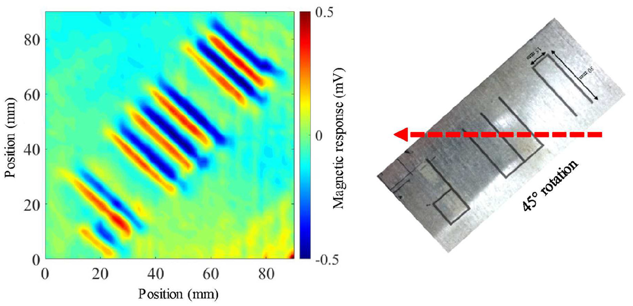
Magnetic map of the steel plate with “UMP” slits using the ECT probe where the letter direction is rotated to 45° with respect to the ECT probe in 2-D.

Backside crack evaluation for sample with different depth

To evaluate the sensitivity of the probe for the backside defect detection, a backside detection measurement was performed with the test sample having the different depth of slits from 1.0 to 1.8 mm. The width of the crack was constant at 1 mm. In this experiment, the slits were positioned at the back of the plate, and the probe was positioned at the front surface.

A line scanning was performed with different frequencies of the excitation field. It was found that the signal intensity was significantly changed at the position of the slits. Even though the signal pattern was not as good compared to the front surface scanning, but the slits could still be detected by the ECT probe. Since the line scan was performed at the 1-kHz excitation field, it could be assumed that the use of the high-frequency field would result in a lower signal-to-noise ratio compared to the lower frequency field. This case was inverse with the surface scanning results, where most of the eddy currents concentrated on the surface and made the ECT probe to detect a higher signal.

The correlation between slit depth and differential signal for the case of the backside measurement was almost the same as the surface measurement and could be observed from Figure 17. Contradict to the surface measurement, the signal showed the lowest value when the excitation was 1 kHz compared to the other frequencies. This due to the skin depth effect where the frequency was inversely proportional to the depth of penetration; hence a smaller magnetic response was reflected at the high-frequency field in Figure 17.

Figure 17.

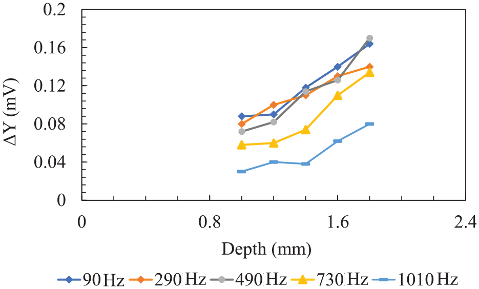
Signal difference of the different slit depths at different frequencies (backside).

From Figure 17, the delta values, which were calculated from the difference between the peak and trough, increased with respect to the depth. The figure above concluded that the pattern was almost linear with respect to the frequency. Since the scanning measurement was performed at the backside, therefore, using a low-frequency field was better than a high-frequency field for the backside defect detection.

Conclusion

In this study, the ECT method was applied to detect a sub-millimeter surface defect and backside defect. Although the ECT method was commonly applied to non-ferromagnetic materials such as aluminium, this study aimed to apply it to ferromagnetic materials such as the galvanized steel plates. For this reason, an eddy current probe using differential AMR sensors has been developed for a sub-millimeter detection of the artificial flaws on the galvanized steel plates.

The developed ECT probe was validated during the detection of the sub-millimeter slits on each of the ferromagnetic carbon steel plates. The results obtained using the developed probe showed that slits could be detected and identified down to 210 µm in depth and 50 µm in width.

Moreover, from magnetic response distribution maps, it was found that the different parameters of the slits would give a different signal characteristic where slits with a perpendicular direction to the probe differential direction would produce a better detection compared to the parallel slits. Moreover, in the case where perpendicular and parallel slits existed together, slits with a longer dimension would be easily identified from the magnetic response distribution maps.

As a future recommendation, an improvement in the design of the probe can be suggested so that defects in any orientations can be detected. Moreover, to make the probe becomes more sensitive to distinguish the tiny size of the defect, the area of the coil needs to be reduced so that the eddy current can concentrate in a small area. ¹³ Future work should also focus on various types of defects and develop a superior system that can be applied and be robust enough to operate in the toughest of environments.