
Abstract
Traditional theoretical calculations, field measurements, and finite element methods sometimes fail to realize life cycle simulations of the temperature field and temperature effect of steel–concrete composite bridge deck systems. In this paper, a simulation method based on a back propagation–long short-term memory (BP-LSTM) network correlation model is proposed to predict the temperature field and temperature effect in a low-cost and highly efficient manner. A bridge was used as the engineering background according to a health monitoring system, and the finite element method based on the principle of heat transfer was used to expand the data sets. Data sets with structural, time, and environmental characteristics as the independent variables and temperature and the temperature effect as the dependent variables were formed. The correlation between the dependent and independent variables was verified using the maximal information coefficient. Thus, the BP-LSTM model was established, and the mean squared error loss function considering the time weight was designed. The data set was read in for training, verification, and testing, and a correlation model representing the relationship between the set’s independent and dependent variables was obtained with relatively high accuracy. Finally, combined with the bridge’s historical meteorological data, the established correlation model was used to simulate the bridge’s temperature field and temperature effect. The results indicated that the finite element calculation results of the structure’s temperature field based on the heat transfer principle were basically consistent with the measured results. The independent variables in the data set were non-linearly related to the dependent variables. The BP-LSTM’s prediction accuracy of the temperature field and temperature effect was above 98.8% and 94.5%, respectively, in good agreement with the target value. The variation law of the temperature field and temperature effect of the steel–concrete composite bridge deck system simulated by combining the historical meteorological statistics was in accordance with reality.
Keywords
Introduction
A temperature load with complex time-varying properties acts on the whole life cycle of a bridge structure, whose temperature field is related to its geographical location, ambient temperature, wind speed, sun radiation, thermal conductivity, heat exchange coefficient, specific heat, emissivity, and other material thermal parameters.1,2 To consider the most adverse temperature effects, fatigue, and other long-term accumulation processes in the design reference period, it is particularly important to simulate the temperature field and temperature effect of the whole life cycle of the structure to design a steel–concrete composite bridge deck system.
At present, the relevant research mainly focuses on the temperature and temperature effect of solely concrete or steel bridges, which are not universal; hence, the conclusions are not completely applicable to steel–concrete composite structures. Tayşi et al. 3 have studied the temperature distribution and time-varying characteristics of concrete beams under the action of ambient temperature based on the full-scale test model and finite element method of box beams. Riding et al. 4 have provided a calculation method for the temperature field of mass concrete considering radiation, material thermodynamic parameters, sunlight shielding, and other factors. Wang et al. 5 have established a temperature gradient model of a steel–concrete composite bridge deck system based on health monitoring temperature data and carried out research on the structure’s temperature effect by combining the model with the spatial finite element method. Tao 6 has established a numerical model of steel–concrete composite beams based on the heat transfer principle and analyzed the relationship between the ambient temperature and structural temperature field considering material properties. At present, the calculation methods of temperature and temperature effect mainly include the following: (1) Converting the overall temperature change based on the annual statistical temperature extremum and then calculating the vertical and horizontal temperature gradients;7–9 (2) introducing the measured temperature field results and using the finite element model to calculate the temperature effect value; 10 and (3) calculating the temperature and temperature effect based on a finite element thermal–mechanical coupling analysis. 11 Among these methods, method (1) fails to reflect the time-varying characteristics of the temperature and temperature effect in the structure’s entire life cycle and does not consider the influence of different geographical location factors on the temperature field. Moreover, method (2) requires long-term measurement to obtain structural temperature data, which is time-consuming and costly. Due to the recent appearance of steel–concrete composite bridge deck systems, there are currently almost no measurement results spanning several decades. The measured points are relatively sparse regarding the cross-section and, thus, cannot accurately reflect its temperature field distribution. Lastly, method (3) can be used for short-term calculations; however, whole life cycle calculations require a supercomputer to realize the massive data computations, so the cost is too high.
In view of the shortcomings of the above methods, a life cycle simulation method of the temperature field and temperature effect of a steel–concrete composite bridge deck system based on back propagation–long short-term memory (BP-LSTM) networks is proposed in this paper. Using the mid-span section of a steel truss stiffening suspension bridge as an example, the “influence parameter – temperature and temperature effect” data set of a steel–concrete composite bridge deck system is established, and the FEM is used to expand the data set based on the measured data. Then, the network structure of the BP-LSTM model is designed to check the correlation of each parameter of the data set, and the network is read into the data set for training, verification, and testing. Finally, the model with the most precise BP-LSTM (after training and passing the test) is selected to realize the life cycle simulation of the structure’s temperature field and temperature effect through historical meteorological parameters. This method combines the advantages of a single traditional method, introduces neural networks based on monitoring data, and achieves the life cycle simulation of a temperature field and temperature effect applicable to China’s climatic characteristics and regional differences between air temperature and sunlight in a cost-effective manner. Moreover, it provides a reference for calculating the temperature and temperature effect of steel–composite structures, analyzing the temperature fatigue effect, and monitoring structural health.
Temperature field monitoring and data set construction of steel–concrete composite bridge deck system
Health monitoring system
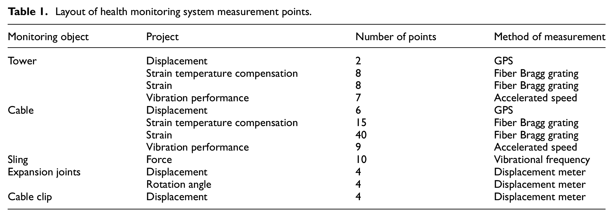
Herein, the main span of the suspension bridge adopted the form of a simply supported steel truss stiffened beam. The roadbed width was 24.5 m, the design speed was 80 km/h, and the bridge deck was a steel–composite structure. An automatic data acquisition system was adopted to monitor the state of the bridge superstructure. The measuring point arrangement is shown in Table 1, and the layout of the measuring points of the mid-span section is shown in Figure 1. Points W1 and W6 were 4 cm from the top of the concrete bridge panel; W2, W4, and W7 were 4 cm from the bottom of the concrete bridge panel; and W3, W5, and W8 were located at the bottom of the steel truss. The measuring points of g1 and g2 were on the same side as the measuring points of W1. Those of g5 and g6 were on the same side as the measuring points of W6, and those of g3 and g4 were to the lower left of the measuring points of W4. L represents the distance between two measuring points of the steel beam. For g1–g2, L = 608 mm; for g3–g4 and g5–g6, L = 838 mm.
Layout of health monitoring system measurement points.
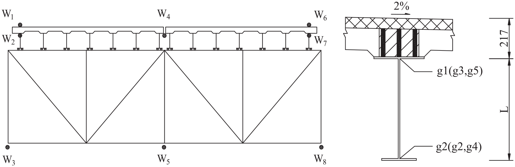
Arrangement of temperature measuring points in mid-span section (units: mm).
Based on the health monitoring system, real-time temperature monitoring was conducted at the measuring points shown in Figure 1. Due to the high sampling frequency, a large amount of temperature data was collected in 2013. According to the method used by Ding et al., 7 it was believed that the temperature values of the measuring points within the unit time length did not change. Thus, the average of these values was taken as the real-time temperature of the measuring points within the unit time length.
Data set construction and expansion
By combining the temperature data collected by the health monitoring system with the statistical data of the National Meteorological Information Center (NMIC), a measured data set containing the time, ambient temperature, and temperature of the measuring points was constructed. However, the actual measuring points were sparse compared with the mid-span section’s size, and the temperature effect could not be directly obtained by the strain sensor of the main beam. For the temperature field and temperature effect problem, many studies have used the FEM based on the heat transfer principle, as the results are in good agreement with reality and can reflect a structure’s actual temperature and temperature effect to a certain extent.3,12,13 Therefore, the FEM was considered to expand the existing measured data set in this study.
FEM model based on the heat transfer principle
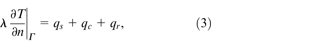
Considering that the full life cycle assessment of a steel–concrete composite bridge deck system mainly concerns the state after the bridge’s completion, that is, once the concrete hydration heat has been completed, the role of the heat source within the structure is not considered. According to the Fourier law and the law of conservation of energy,13–15 the partial differential equation of heat conduction can be written as:

where
The heat conduction partial differential equation establishes the space–time relation of the internal temperature of the structure. If the definite solution conditions (initial and boundary conditions) are introduced, the solution can be solved simultaneously with this equation. The initial condition refers to the temperature field at the initial moment of the steel–concrete composite deck system, which can be expressed as:

Under the action of sunlight, the heat exchange paths between the steel–concrete composite bridge deck system and the outside world mainly include the heat flow at the boundary of solar radiation, which convects and radiates with the structure and surrounding environment. Its boundary conditions can be expressed as:14,16
where n is the outer normal direction of boundary
Based on the research of Kehlbeck,
17
a power exponent model was used to calculate the direct radiation intensity reaching the Earth’s surface, and then the density of solar radiation heat flux,
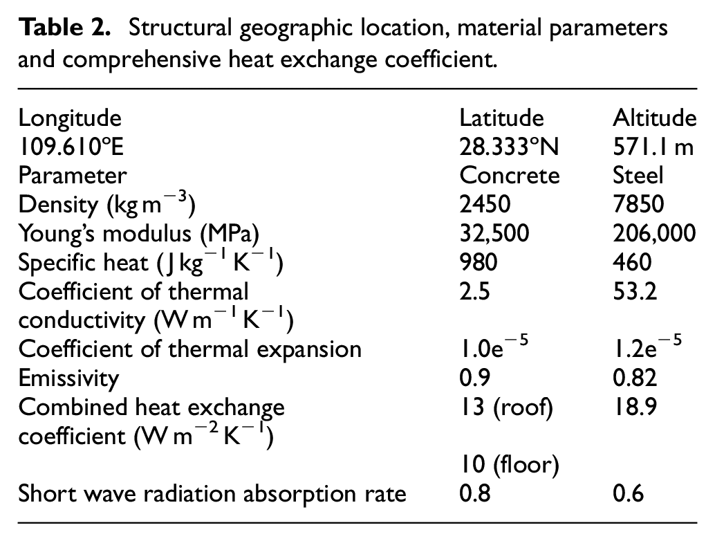
According to the statistical data of the daily ambient temperature at the NMIC’s bridge site in 2013, 4 days were sampled in each month of the year. Based on the above heat transfer principle, the structure heat transfer boundary conditions were calculated using Python 3.6. The FEM model was established by ABAQUS for the thermo-mechanical coupling analysis. Before conducting the structural temperature field and temperature effect analysis, an additional 48-h analysis step was added to eliminate the temperature field error at the initial moment of the steel–concrete composite bridge deck system.18,19 The finite element calculation results were verified using the data collected by the health monitoring system. According to Saint Venant’s principle, three standard internode lengths of stiffened beam segments in the main span were selected along the length direction, and the FEM was established using ABAQUS, as shown in Figure 2. For the geometrically regular engineering examples in this paper, using the first-order element can greatly reduce the calculation amount and improve the calculation efficiency on the premise of ensuring the calculation accuracy. In the model, a steel truss beam, steel longitudinal beam of a bridge deck system, and bridge deck slabwere simulated by a three-node three-dimensional thermo-mechanical coupling truss element (T3D2T), eight-node thermo-mechanical coupling shell element (S8RT), and eight-node three-dimensional thermo-mechanical coupling hexahedron element (C3D8RT), respectively, for a total of 210,142 nodes and 164,974 elements. The boundary conditions were applied to four corner points at both ends of the model mileage direction and the position of the lifting point according to the actual structure constraints. The structural geographic location, material parameters, and comprehensive heat exchange coefficient of the heat transfer boundary14,15,20 are shown in Table 2, and the heat flux density of each characteristic surface of the structure is shown in Figure 3 (only partly listed due to the large amount of data).
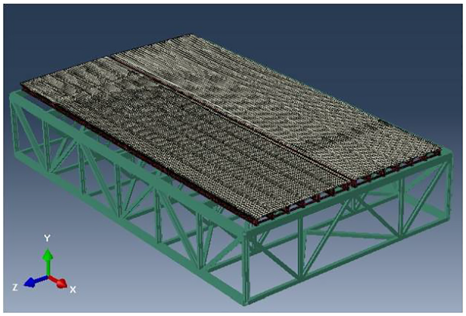
Superstructure finite element model.
Structural geographic location, material parameters and comprehensive heat exchange coefficient.
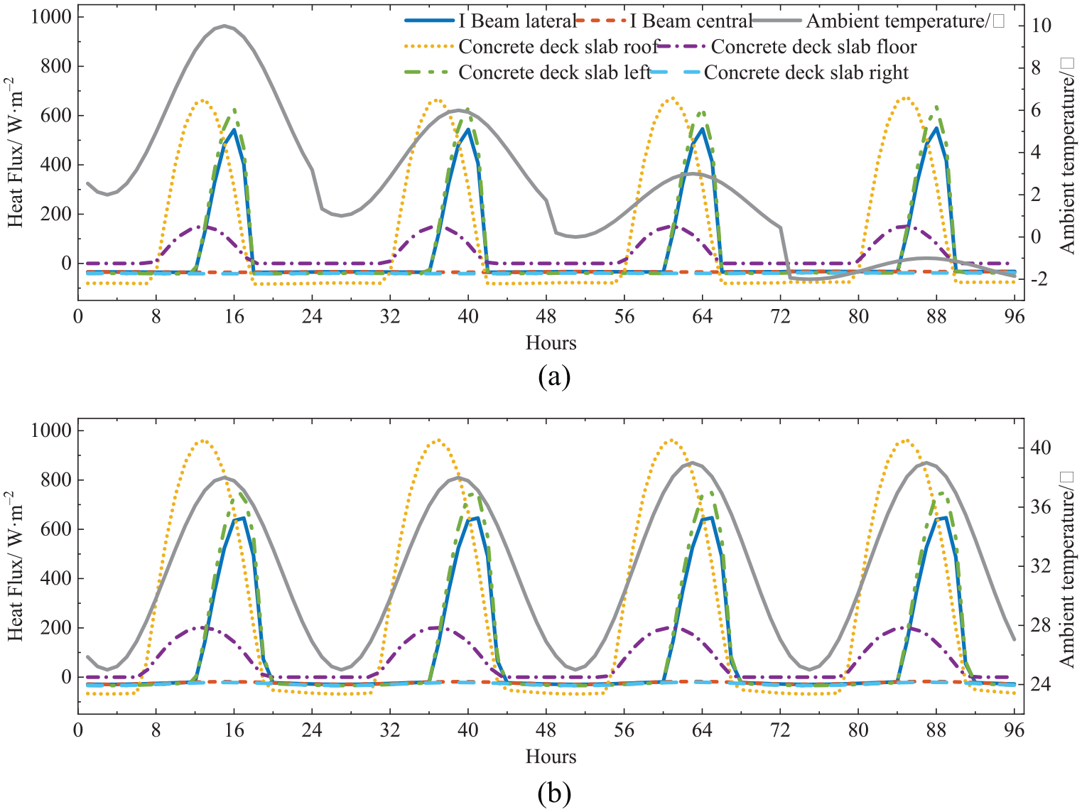
Heat flux on characteristic surface of steel–concrete composite bridge deck system: (a) 2013.1.1–2013.1.4 and (b) 2013.8.10–2013.8.13.
Comparison between the measured values and FEM results
The FEM results were verified using the temperature data at the measuring points on the steel–concrete composite bridge deck system. Owing to limited space, Figure 4 only shows the comparison between the FEM results and measured data at the measuring points on January 1–4 and August 10–13, 2013. In addition, the linear regression method was used to establish the relationship between FEM result
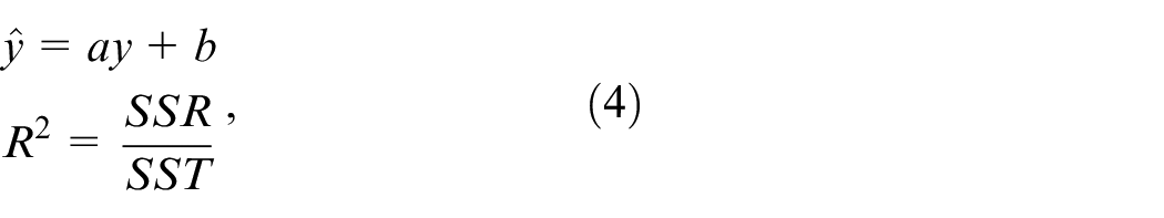
where a and b are the regression coefficients, SSR is the regression sum of squares, and SST is the total sum of squares.
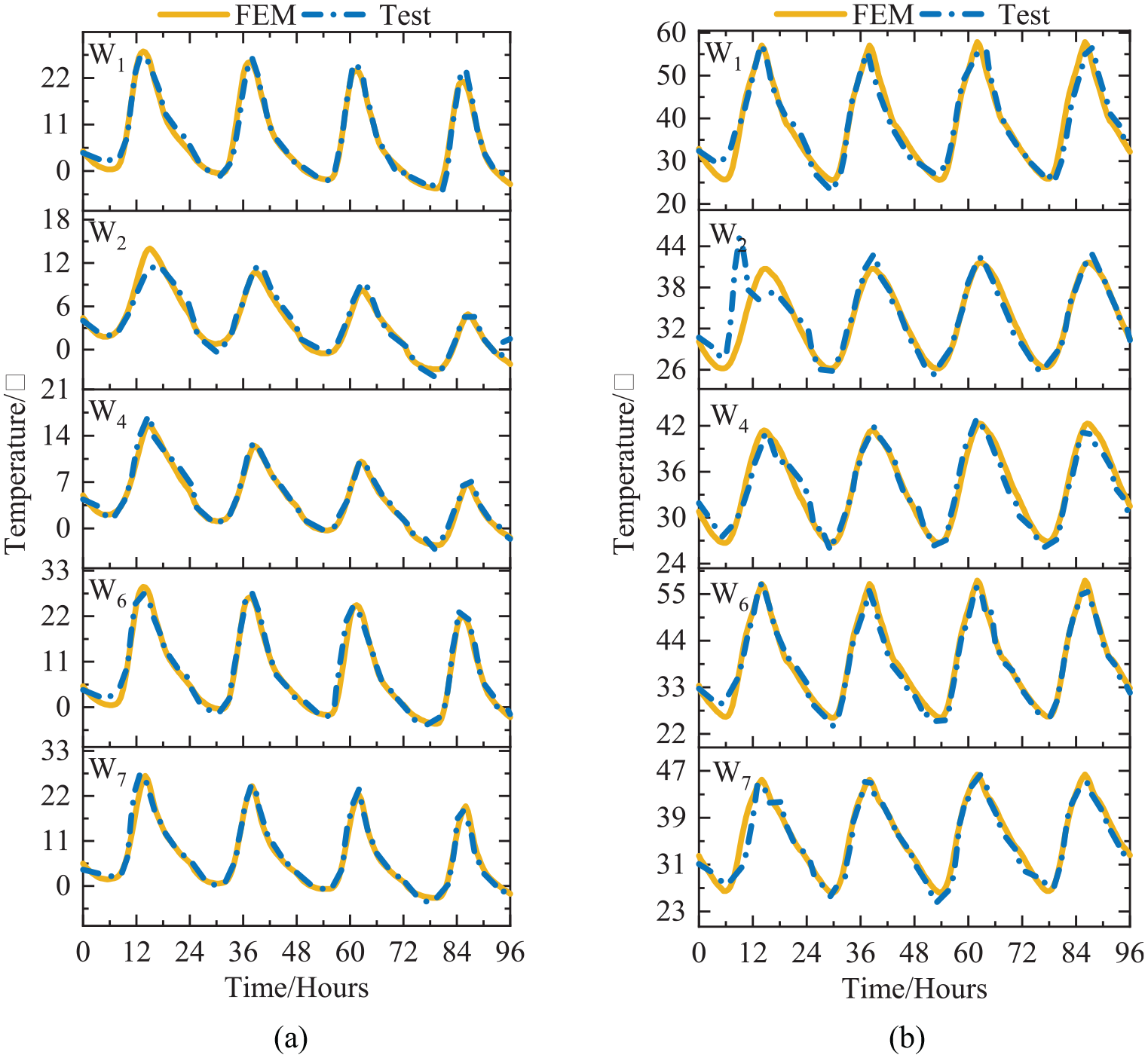
Comparison of the measured values and FEM values: (a) 2013.1.1–1.4 and (b) 2013.8.10–8.13.
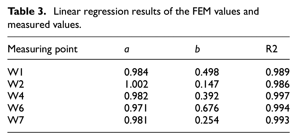
When a = R2 = 1 and b = 0, the FEM results could be considered to be exactly the same as the measured data. The FEM results were linearly regressed with the measured data; the regression results of each measured point are shown in Table 3. Combining Figure 4 and Table 3, it can be seen that the FEM calculation results were basically consistent with the actual measurements. According to the calculated results and measured values at different measuring points, determination coefficient R2 and regression coefficient a approached one, while regression coefficient b approached zero, showing a significant correlation. This indicates that the parameters of the current FEM model were relatively reasonable and that the heat transfer boundary was in line with reality. Therefore, the temperature value and temperature stress value of each node in the FEM model could be used to expand the existing measured data set. (In this paper, the steel-concrete composite bridge deck system is statically determinate structure, and the overall temperature change does not produce the temperature self-restrained stress. Therefore, we only consider the temperature secondary stress caused by the temperature gradient, and it is only related to the relative temperature change of each part of the structure.)
Linear regression results of the FEM values and measured values.
Data set expansion
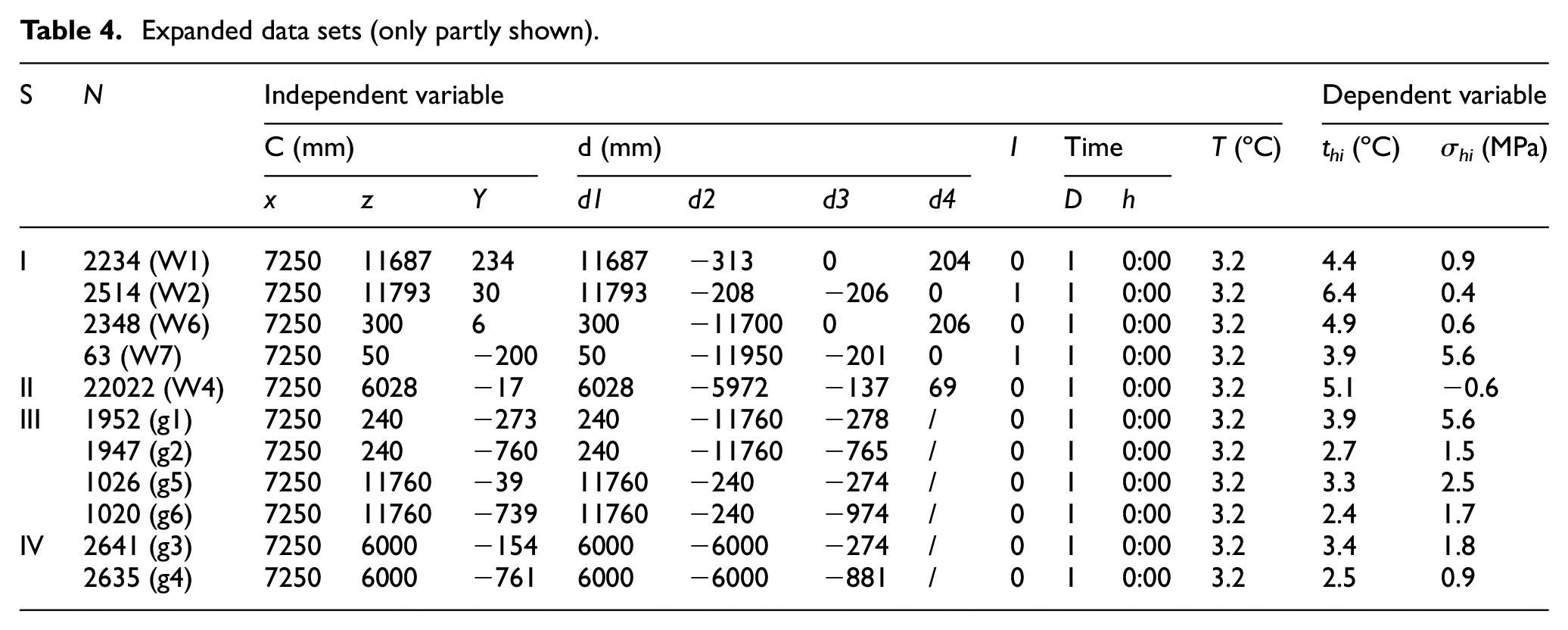
Using the FEM combined with meteorological data, the temperature and temperature effect at any position in the steel–concrete composite bridge deck system at any time could be calculated. Since the above data set was only for this bridge, its geographical latitude and longitude (ignoring the difference in longitude and latitude of each location of a single bridge structure), material density, heat exchange coefficient, emissivity, thermal conductivity coefficient, and specific heat were constant. The variables that affected the surface heat flux density were mainly the differences in the day ordinal, moment ordinal, and ambient temperature and the normal vector of each surface space. Thus, we could expand the data set. As shown in Figure 5, structural, time, and environmental characteristics were used as the independent variables, and temperature and temperature effect were used as the dependent variables. The variable container dictionary in Python was used for the input and classification management. In Figure 5, S represents the node type (external surface (I), internal (II), side beam (III), medium beam (IV)), N represents the node number, Cx, Cy, and Cz represent the node coordinates in three axes’ direction components, d1, d2, d3, and d4 represent the distance between the node position and the upper, lower, left, and right surfaces, respectively, I represents the contact between steel beam and concrete at the joint position (“0” means no contact, “1” means contact), D represents the day ordinal, h represents the moment ordinal, T represents the ambient temperature, thi represents the temperature value of node i at time h, and σ hi represents the temperature effect value of node i at time h. Using the measuring point in Figure 1 as an example, its expanded form according to Figure 5 is shown in Table 4. Take the section at the mileage x = 7250 mm as an example, the 48-feature day hourly database of each node of the section is 1,368,756 × 15 table, and only part of the data is given due to the limitation of space.
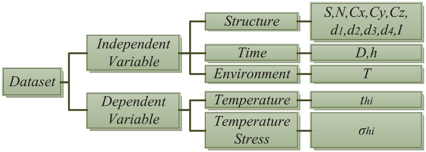
Data set hierarchy.
Expanded data sets (only partly shown).
Life cycle simulation of temperature field and temperature effect
Based on the established data set, the following method was used to verify the correlation of all data, seek characterization methods, and realize the life cycle simulation of the temperature field and temperature effect of the steel–concrete composite bridge deck system:
A correlation test was performed for all variables in the data set to clarify their correlation, and the test results were screened according to the actual requirements.
A BP-LSTM hybrid model was constructed, and the model parameters with the highest accuracy were retained through training and testing.
(3) Meteorological data were introduced to generate read-in data, and the BP-LSTM hybrid model was used to predict the temperature field and temperature effect.
Correlation test
Based on the constructed data set containing structural, time, and environmental characteristics as well as the temperature and temperature stress of the measuring points, the temperature and temperature effect values of the nodes at the specified time and ambient temperature were obviously unique. Moreover, there was a mapping relationship between the independent and dependent variables in the data set. The maximal information coefficient (MIC) method was adopted as the feature selection method, as it can effectively evaluate the correlation between different data on the basis of equity. 21 Its basic steps were as follows: (1) Random variables X and Y were sorted to form the data set; grid nx × ny was divided, and the mutual information value of the two variables was calculated to obtain the maximum mutual information value, Im (Formula 5). (2) The maximum mutual information value was normalized (Formula 6), and that same value at different scales was selected as the MIC value (Formula 7).
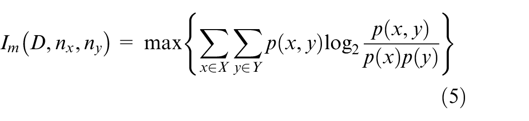
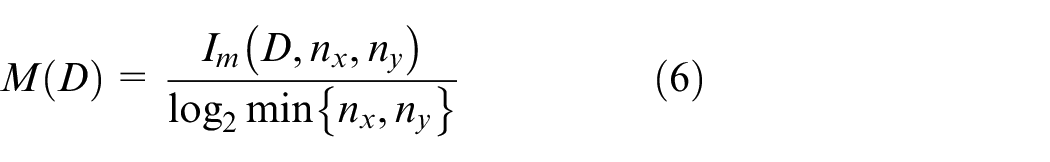

where B(n) represents the grid resolution, which is usually the 0.6 power of the data volume.
Regardless of S, N, and I in the above data set (because node type S and node number N in the data set are only identifiers and I only has two values of 0 and 1), the correlation values of thi, σ hi , and each input feature were calculated, and matrix visualization was performed, as shown in Figure 6.
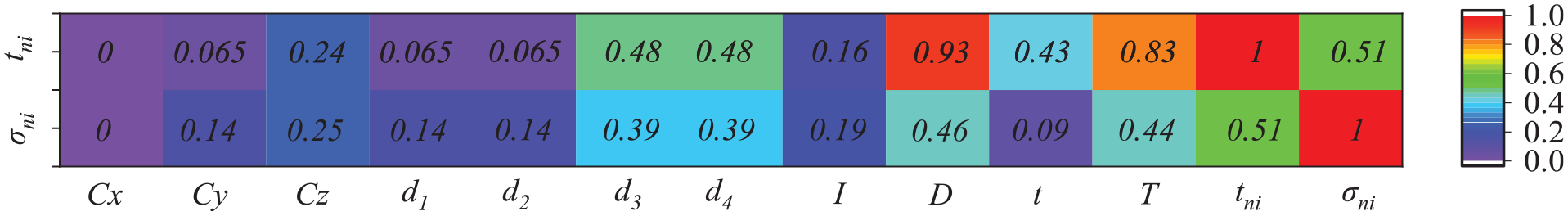
The MIC matrix heat map of the temperature, temperature effect, and each dependent variable.
The matrix heat map showed that the temperature and temperature effect had a nonlinear correlation with each input, except autocorrelation. Since the current data set was only for the cross-section with measuring points in the span and distance coordinate Cx of the cross-section was a constant value, MIC = 0; if the data set contained cross-section data with different distances, then MIC ≠ 0.Moreover, the node temperature was highly correlated with the distance between the nodes and the upper and lower surfaces as well as the day ordinal, moment ordinal, and ambient temperature. The node temperature effect was highly correlated with the distance between nodes and the upper and lower surfaces as well as the day ordinal and ambient temperature. Meanwhile, thi and σ hi had a weak correlation with the transverse coordinates of the nodes, consistent with the general cognition. It can be seen that the correlation shown by the MIC was relatively reliable. It was difficult to use a simple elementary function to describe the above correlation, so a neural network was introduced to realize the representation of the above nonlinear relation.
BP-LSTM hybrid model construction
The BP neural network is the most widely used artificial neural network (ANN) structure. It adopts the BP algorithm and consists of an input layer, a hidden layer, and an output layer. It can describe any mapping relationship without corresponding equations. The universal approximation theorem proposed by Hornik et al. 22 and Cybenko 23 demonstrates that feedforward neural networks can fit functions of arbitrary complexity with arbitrary precision with only a single hidden layer and a finite number of neurons. The basic BP algorithm includes forward propagation of signals and BP of errors:


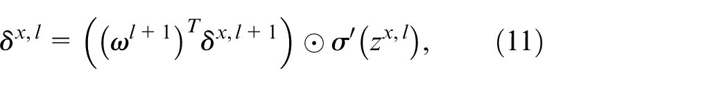
where
An LSTM network is a circular structure of network chaining proposed by Hochreiter and Schmidhuber 24 in 1997 to solve the long-term dependence problem of traditional recurrent neural networks (RNNs). It controls the network input through the input gate, the memory unit through the forgetting gate, and the network output through the output gate. Due to its unique structure, the time series problem can be processed and predicted. The basic LSTM algorithm is shown below:


where
Structure of the BP-LSTM
For the aforementioned established data set, its ambient temperature, measuring point temperature and temperature effect, day ordinal, and time ordinal were obviously chronological. Because there was no connection between the nodes in each layer, the BP network could not remember the network’s past output value, so it had poor predictive ability for the time series problems of coherence. Moreover, it was difficult to simulate the temperature and temperature effect of the steel–concrete deck system with high precision. The LSTM is a variable network based on RNN with a good ability to deal with long time dependence problems. However, it needs a lot of training data, and the predicted value at time t will be affected when there is a deviation in the predicted value at time t − 1. For long-term prediction problems, a large deviation often occurs in the middle and back parts of the prediction sequence. To solve these problems and give full play to the advantages of the two types of ANNs, a BP-LSTM hybrid model was proposed herein. Its basic structure is shown in Figure 7. Its cell structure, forgetting gate, input gate, and output gate were consistent with the typical LSTM structure; At, xt, Ct, and ht represent the LSTM network unit, input vector, cell state, and output vector, respectively. At time t, output vectors Ct−1 and ht−1 of the hidden layer at the previous time t − 1 and input vector

where
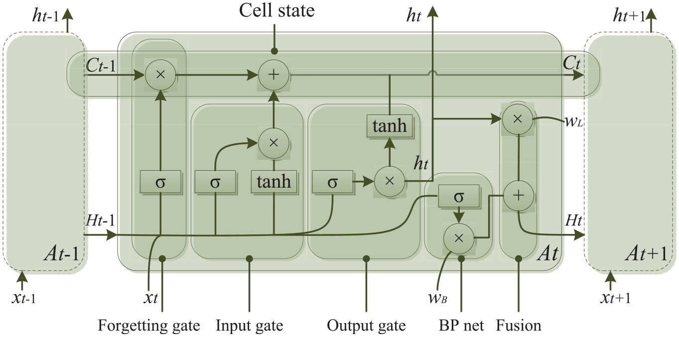
BP–LSTM network structure.
Data preprocessing
To avoid the occurrence of singular sample data, which may cause a lengthy training time, gradient explosion, or network convergence failure, the Z-score method was selected to normalize the data set:
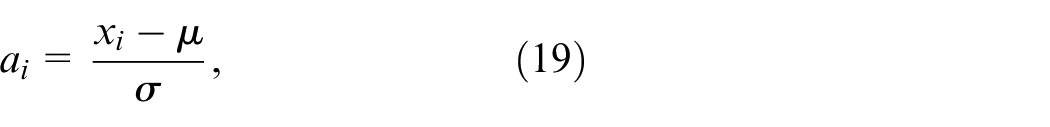
where
After normalizing the data, two copies of the same sample were generated and randomly disturbed. According to the proportion of 70%:15%:15%, the data was divided into a training group, a verification group, and a test group. Moreover, {S, N, Cx, Cz, Cy, d, I, D, t, T} was used as the input value and {thi, σ hi }as the target value. The Pytorch deep learning framework was utilized to transform the data types, and function DataLoader of Pytorch was used to define iterators to realize random mini-batch training.
Activation function and loss function
Since the above problem was a regression problem, the activation function in the output layer adopted the identity function, while the activation function in the hidden layer adopted the ReLU function. (The traditional Sigmoid and Tanh functions have problems of gradient descent and stop learning when the output is saturated, and the gradient disappears when the weighted input is negative, while the ReLU function solves the above problems well.) When the number of nodes in the previous layer was i, the initial value used the Gaussian distribution with a standard deviation of
The loss function represented the “bad degree” of ANN performance, that is, the underfitting degree of target data by the current ANN. Common loss functions include mean square error (MSE), mean absolute error, and cross entropy error. For the BP network, the most common MSE was selected here as the loss function:

where C is the loss function,
For the LSTM, considering that the network input was an equal-length sequence after filling and that the actual effective length of each sequence was different, it was obvious that time weight factors should be set for the sequences with different time lengths to avoid unreasonable adjustment of the weights and biases of each network layer due to the small amount of data of the short sequence in the input. The time weight factor was introduced based on the MSE to use the improved MSE as the loss function:
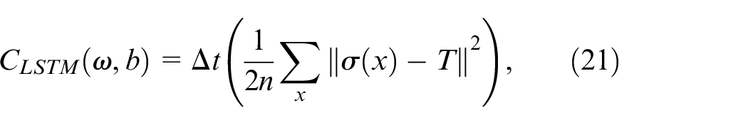
where in time weight factor
Time weight factor is equivalent to simulate a human brain on memory process of forgetting, by introducing it, the influence of input data close to the predicted time on the predicted result could be increased. However, ordinary MSE function is not sensitive to time series and does not consider the difference of results generated by different occurrence times of events.
Super parameter setting and network training
For the BP and LSTM networks, dropout, mini-batch, batch normalization, and early stopping were adopted in the training phase to achieve the optimization results of precision and overfitting inhibition. The dropout randomly deleted neurons during the training process to suppress overfitting. 26
Considering the large amount of network input data, especially for the LSTM network, sequences of different lengths had to be constructed and supplemented to the same length, and the time complexity of the computation showed an increase of O(n2). Owing to the limitation of hardware resources, mini-batch training was introduced to improve the computing speed and accelerate the network convergence. 27 The batch normalization normalized the mini-batch during the network training to accelerate the network convergence, weaken the initial weight dependence, and suppress overfitting. 27 The early stopping calculated the loss function for the verification group in each calculation cycle. When the value of the loss function kept rising, the training stopped, and the best network parameters in all training cycles were output to suppress overfitting and reduce the training time. 27 The Adam method 28 was adopted as the optimization method; the hyper-parameters are shown in Table 5 (lr is the learning rate, β1 and β2 are the primary and secondary momentum coefficients, respectively, of the Adam method, S is the batch size, dr is the neuron deletion ratio of the dropout, wB is the output weight of the BP network, and wL is the output weight of the LSTM network; lr, dr, wB, and wL were determined by trial calculation. β1 and β2 were the recommended coefficients for ADAM-method. S was related to computer hardware configuration, and different batch-size could be adopted according to different configurations, which mainly affected the model training speed).
Hyper-parameter values.

After all parameters were set, the BP-LSTM was trained using the independent variable in the data set as the input value and the dependent variable as the target value. After repeated cyclic training, the model parameters with the minimum loss function and the highest accuracy were retained and loaded in the test stage.
Evaluation of reconstruction and generalization ability and comparison with independent model prediction results
The error between predicted value y and target value T of the BP-LSTM model was evaluated by determination coefficient R2, and relation T = ay+b was established by the linear regression method; a and b were the regression coefficients. The training results and probability distribution of temperature thi and temperature effect σ hi are shown in Figure 8. (It should be pointed out that the total data set reached 1,368,756 rows. After the training group, verification group and test group were divided according to the proportion of 70%:15%:15%, the data amount of each group was still large. Only a small number of points deviated from the straight line y = T in Figure 8(a) and (b), and most of the other points were located near y = T. The distribution difference between the predicted value and the target value is shown in Figure 8(c). The consistent distribution of the two values and the higher determination coefficients of the training group, the verification group and the test group all indicate the consistency of the predicted value and the target value.)
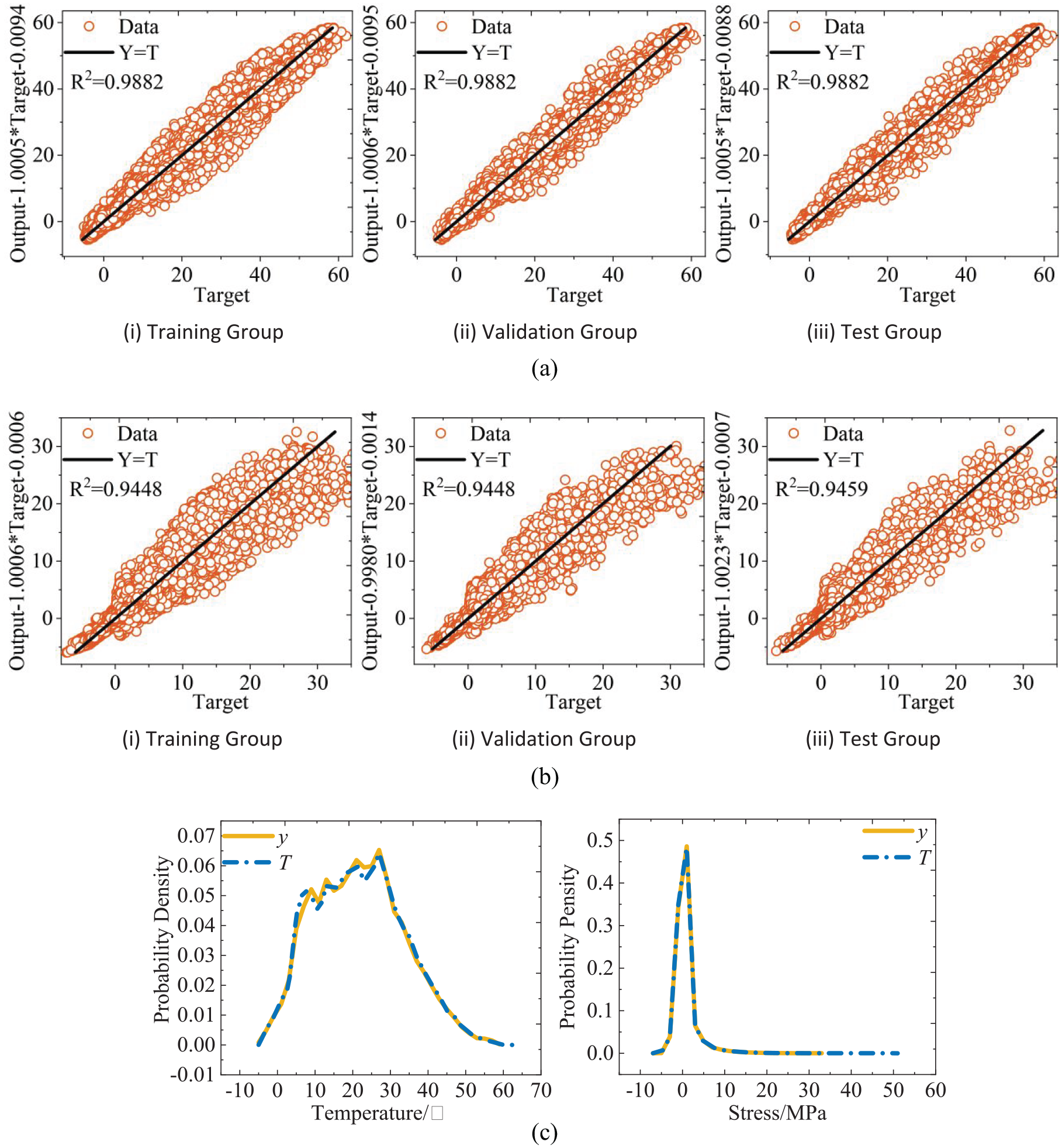
Training results of temperature thi and temperature effect σhi in the BP-LSTM model: (a) temperature,
As can be seen in Figure 8(a) and (b), the model performed well in the training, verification, and test sets. The distribution of the temperature and temperature effect in all sets was relatively consistent. Determination coefficient R2 and regression coefficient a tended toward 1, while b tended toward 0, indicating that the network had a strong reconstruction and generalization ability. Coefficient R2 ≈ 0.945 of the temperature effect was slightly lower than that of the temperature, indicating that the temperature prediction accuracy of the current prediction model was better than that of the temperature effect. In Figure 8(c), the predicted value and target value probability density distributions of the temperature and temperature effect were almost the same, also suggesting that the prediction accuracy of the current BP-LSTM model was relatively high.
The BP-LSTM training data set was used to train the independent BP and LSTM models respectively. The prediction results of the independent model and the hybrid model for the same input data are shown in Figure 9. (In order to make the comparison clearer, only the partial prediction results of nodes at the intersection of concrete roof and left side web are shown.) It can be seen that the independent BP and LSTM models are not ideal in predicting temperature and temperature effect, while the mixed BP-LSTM model is more accurate in predicting results.
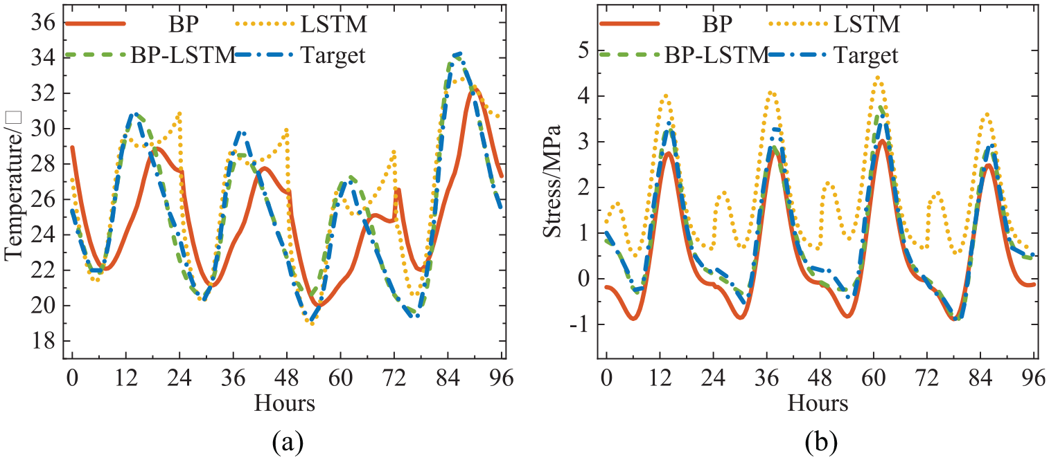
Comparison of 8.10–8.13 prediction results of BP, LSTM and BP–LSTM: (a) temperature and (b) temperature stress.
The above results confirmed the reconstruction and generalization ability of the BP-LSTM model. The temperature and temperature stress of each node could be generated according to the specified structural, environmental, and time parameters with high accuracy and could be used in the life cycle simulation of the temperature and temperature effect of the steel–concrete composite bridge deck system.
Life cycle simulation
The above BP-LSTM model successfully established the mapping relationship between the independent and dependent variables. For the whole life cycle of the steel–concrete composite bridge deck system, the structural and time characteristics of the independent variables were known. If the change in ambient temperature could be accurately predicted, the temperature and temperature effect value of a structure throughout its whole life cycle could be accurately calculated. However, it is impossible to predict ambient temperature in the long term. However, according to the viewpoint of Ding et al., 29 historical ambient temperature data can be used to replace the predicted value of ambient temperature within a structure’s whole life cycle. It should be pointed out that basic meteorological statistics have been available in most parts of China since 1950 and that relevant data have been available for about 70 years and are representative to a certain extent. According to Ding et al. 29 and Yu’s 30 study, since 1951, China’s annual average temperature and other indicators have changed somewhat, and the average surface temperature in the country has risen by about 0.5°C–0.8°C within nearly 100 years. In the central China area wherein the bridge is located, the decrease of the minimum average daily temperature in summer is about −0.1°C/10a, and the maximum average daily temperature basically remains unchanged. Moreover, the increase of the minimum average daily temperature in winter is about 0.4°C/10a, and the maximum average daily temperature increase is 0.2°C/10a. Relative to the bridge structure, the overall average annual temperature and average daily temperature change little, and the influence on the temperature field and temperature effect of the bridge deck system can be ignored. Therefore, we can assume that the temperature statistics since 1950 in the probability distribution are consistent with the temperature data of the future service life of the bridge. The temperature field and temperature effect in the bridge’s future service life can be predicted based on the statistical law of meteorological data in the bridge site area in past decades.
After inputting the temperature data of the bridge area collected by the NMIC into the BP-LSTM model, the temperature and temperature effect at each position of the mid-span section of the steel–concrete composite bridge deck system over 60 years were output. Due to limited space, only the prediction results of the BP-LSTM model for measuring points W1, W2, W4, W6, and W7 and steel beam points g1–g6 from 2012 to 2019 are given in Figure 10.
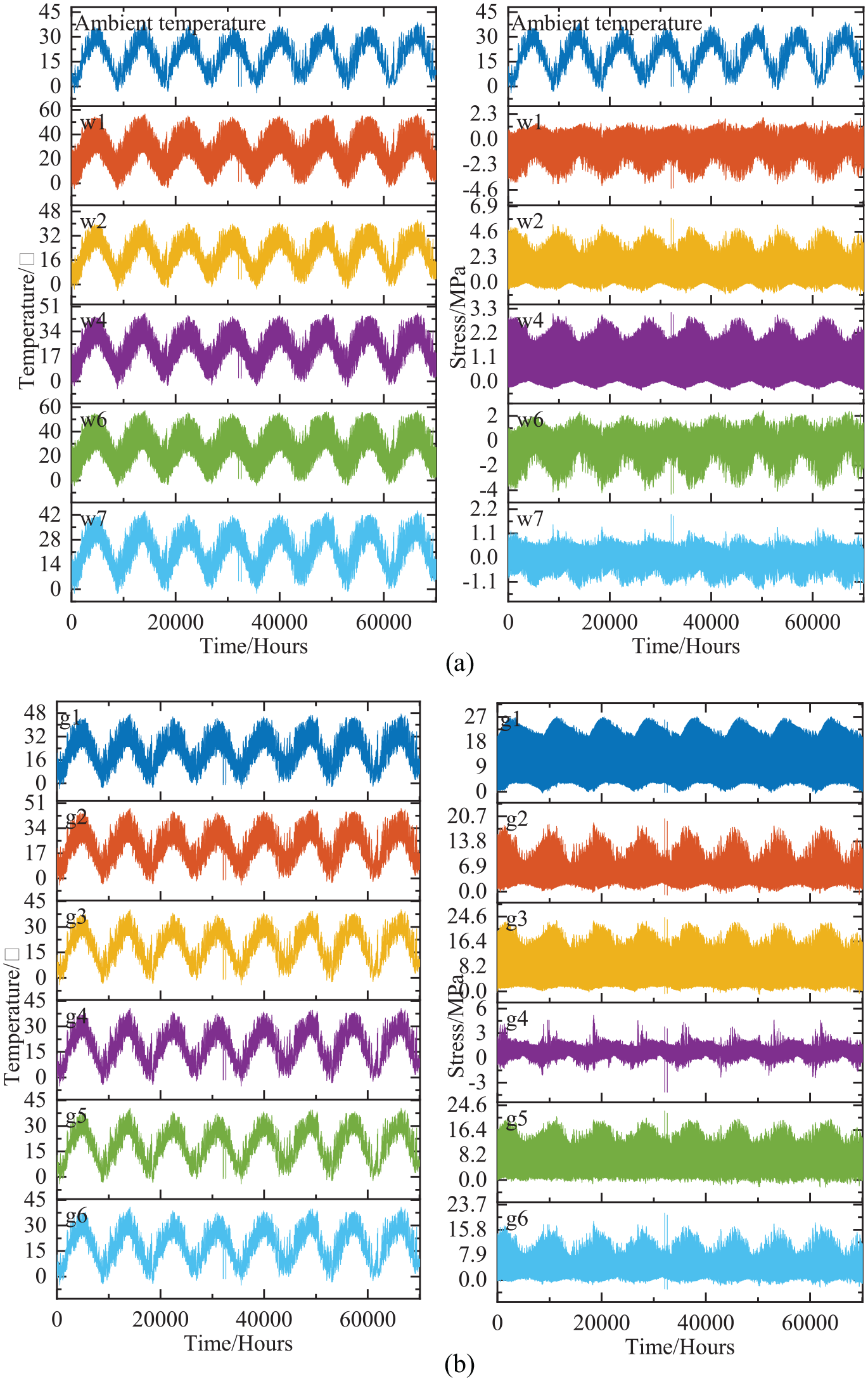
Temperature and temperature effect simulation of the steel–concrete composite bridge deck from 2012 to 2019: (a) concrete measuring points and (b) steel beam points.
In the prediction results, the temperature changed significantly as the meteorological temperature changed over the four seasons, consistent with the general cognition. The maximum and minimum temperatures of the concrete bridge panels were 57.3°C and −5.3°C, respectively, and the maximum and minimum principal stresses were 5.8 and −4.5 MPa, respectively. The maximum and minimum temperatures of the steel longitudinal beams were 47.6°C and −5.1°C, respectively, and the maximum and minimum values of von Mises stress were 27.0 and −4.2 MPa, respectively. The indexes of the temperature and temperature effect were within a reasonable range, and the variation trend was reasonable, which well reflected the variation characteristics of the temperature and temperature effect of the steel–concrete composite bridge deck system. (It should be pointed out that when the time was in the interval of [30,000, 40,000], the abrupt change of ambient temperature in part of the time period caused the change of heat flux on the surface of the structure, which led to the change of structure temperature. When the ambient temperature with sudden change is input into the FEM model, the change of the structure temperature is basically consistent with the sudden change in the Figure 10. The occurrence of such abrupt change was well predicted by the BP-LSTM hybrid model, which further verifies the correctness of the method presented in this paper.)
Conclusions
The temperature field and temperature effect of a steel–concrete composite bridge deck system under complex environmental conditions are important foundations of the system’s whole life cycle performance design. In this study, the mid-span section of a steel truss stiffening suspension bridge was used as an example. Based on the measured results and FEM simulation, the data set was composed of structural, time, and environmental characteristics, the temperature field, and the temperature effect. On this basis, the life cycle simulation method of the temperature field and temperature effect of the steel–concrete composite bridge deck system based on a BP-LSTM hybrid model was proposed. The analysis results indicated that:
The FEM calculation results based on the heat transfer principle were close to the measured temperature field, so the FEM method could be used to expand the measured data and generate a data set with a long time span and comprehensive measuring point positions.
The MIC was used to analyze the data set, and its analysis results showed that the temperature and temperature effect were strongly correlated with the structural, time, and environmental information. Moreover, the correlation of each variable was consistent with the conventional cognition.
The BP-LSTM hybrid model proposed in this paper effectively dealt with the prediction problem considering the influence of the time series. The modified MSE loss function considering the time factor had a good effect; the model had a high precision, and the reconstruction and generalization ability was strong. The life-cycle predicted results were within a reasonable range, and it could provide a reference for temperature load research, temperature fatigue calculation, and structural health monitoring.
Footnotes
Declaration of conflicting interests
The author(s) declared no potential conflicts of interest with respect to the research, authorship, and/or publication of this article.
Funding
The author(s) disclosed receipt of the following financial support for the research, authorship, and/or publication of this article: The research described in this paper was financially supported by the Natural Science Foundation of China (Grant No. 51878072); Graduate Student Research Innovation Project of Hunan Province (CSUST) (Grant No. CX20190661).