Sage Journals: Discover world-class research

Abstract

The equivalent circuit model of pulsed eddy current testing (PECT) has simple mathematics but its applications are limited to qualitative analysis such as principle illustration and signal interpretation. In this paper, the parameters of equivalent circuit model are estimated using system identification method and quantitative relationships are found between some of the parameters and the size of the defect. The equivalent circuit equations were solved from the perspective of system analysis to yield the system transfer function. An m-sequence of 10 order was selected to excite the system and the probe current was used as the output. A set of experiment input-output data for system identification were obtained by performing experiments on two aluminium alloy 6061 slabs, one of which was machined with five slots of different widths, and the other one was machined with five depth-varied slots. The equivalent circuit parameters were finally estimated based on the identified transfer function parameters. It is found that the values of resistance and self-inductance of the secondary windings decrease greatly and monotonically with the increase of the slot width or depth. The self-inductance is more sensitive to the slot size variation than the resistance. Both of them have the potential to serve as the signal feature for defect evaluation in PECT applications.

Keywords

Pulsed eddy current transfer function system identification defect evaluation nondestructive testing

Introduction

The pulsed eddy current testing (PECT), which utilizes a repetitive broadband pulse as its excitation, has gained much attention in the family of eddy current testing (ECT) for decades due to its notable characteristics such as deep penetration in the conductive specimen, diverse time-domain signal features and simple electronics for instrumentation.¹ Originally developed for measuring the thickness of zirconium coating on nuclear fuel elements,² this technique has been extensively used for defect inspection and evaluation, thickness measurement and conductivity characterization.^3–6 By now, PECT instruments have achieved wide applications in the inspection of cracks in multilayer aircraft structure^7,8 and corrosion under insulation.^9,10

Along with the development of application, the modelling approach has also been investigated because it not only helps understand the underlying physical process but also can be used to fast simulate and predict the probe responses without performing toilsome practical inspections, thus providing guidance for the selection of inspection parameters and the design of a probe. Analytical modelling, which is based on the Maxwell’s equations, has the most rigorous derivation and is of great theoretical importance. Almost all present ECT analytical models are originated from the classical model made by Dodd and Deeds¹¹ who derived closed-form integral solutions in the late 1960’s for a coil above a layered conducting half space as well as a coil surrounding an infinitely long conducting rod. For PECT modelling, the algorithms of Laplace transform (LT) and inverse LT (ILT) or Fourier transform (FT) and inverse FT (IFT) were adopted to bridge the transient excitation/response and the harmonic excitation/response.^12,13 Although a lot of studies were reported in the literature, for now, analytical modelling is still restricted to the cases of simple tests geometries and regular shaped defects. Numerical modelling which employs discretization of the solution domain and numerical integration turns out to be a complement to the analytical modelling. With the fast development in computer technology, one can tackle PECT problems with arbitrary shaped defects and specimen geometries by using commercially available numerical simulation software.¹⁴

Another modelling approach, known as the equivalent circuit model or the transformer model, regards the interaction between the probe and the specimen as a transformer. The probe and the specimen are respectively modelled as the primary and the secondary windings, both consisting of a resistance in series with an inductance, and their coupling is described by a mutual inductance. The equations of the equivalent transformer circuit can be established by using Kirchhoff’s voltage law, but how to obtain the unknown parameters involved in the equations becomes the key part of the modelling. Lefebvre et al.¹⁵ used the Levenberg-Marquardt algorithm to curve-fit PECT signals to the equivalent circuit model. Their study showed that choosing adequate initial guess values of model parameters is crucial for solution converging and getting an excellent fit. Vyroubal¹⁶ presented a new transformer model with single primary and multiple secondary windings to calculate the impedance of the eddy-current displacement probe. By dividing the specimen’s eddy current circulation paths into a sufficient number of single-turn rings, good agreement was achieved between the modelled and the measured probe responses.

From the perspective of system analysis, the PECT signal can be regarded as an impulse response of the PECT system. Hence, transfer function as well as system identification were also used to characterize the PECT system. Tondo et al.¹⁷ deduced the transfer function representing the admittance of the probe coil from the equivalent circuit. Then an inductive time constant was obtained from the transfer function parameters and explored as a new feature to assess the size of slots fabricated on a metal sample. Preliminary analysis showed that the inductive time constant is more sensitive than the traditionally used reflected impedance. Dadić et al.¹⁸ proposed a z-domain, finite impulse response (FIR) model along with the least mean squares (LMS) algorithm to identify the response of the PECT system. Lang et al.¹⁹ applied the system identification method to establish the transfer function model of PECT systems. The transfer model was considered to be of second order and the identified model parameters were processed by Fisher discriminant analysis (FDA) to classify defect patterns. In a different way, Lee et al.^20,21 determined the PECT system transfer function between the probe terminal and the instrument readout, so as to deduct instrument dependence from the experimental waveform and thus make the converted waveform comparable to model-predicted or benchmark waveforms.

All in all, compared with analytical modelling, equivalent circuit model or transfer function based model doesn’t involve complex mathematics, but the model parameters were not thoroughly studied in the application of defect evaluation. This paper is concerned with the parameter identification of equivalent circuit model and exploration of new features from identified parameters for pulsed eddy current nondestructive evaluation.

Equivalent circuit modelling

The equivalent circuit modelling is to equate the electromagnetic phenomenon and process as a circuit composed of ideal power sources and circuit elements, and thus conduct circuit analysis instead of field analysis. The working frequency of a typical PECT system is from a few Hz to kHz which belongs to the low frequency regime. This means that the system dimension can be considered as electrically small when compared to the excitation wavelength. Therefore, the electromagnetic coupling between the PECT probe and the specimen can be simplified to a lumped-parameter transformer, as shown in Figure 1. The primary and secondary windings of the transformer represent the probe coil and the specimen under test, respectively. The lumped parameters u₁, R₁ and L₁ in the primary side refer to the pulse source, the coil resistance and the coil inductance respectively, while R₂ and L₂ in the secondary side describe the specimen. The magnetic flux linkage between the probe and the specimen is then described by the mutual inductance M.

Figure 1.

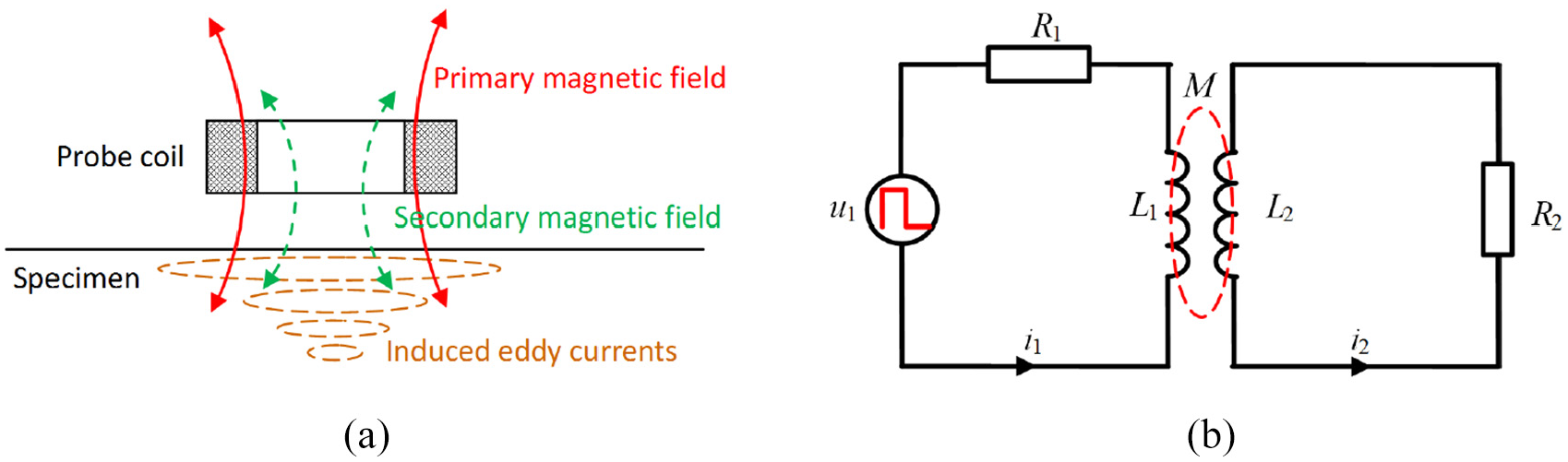
(a) Schematic of PECT and (b) its equivalent circuit model.

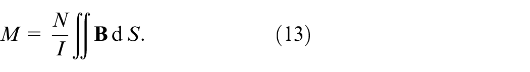
The mutual inductance M between the primary coil and the secondary coil is expressed as

M = k \sqrt{L_{1} L_{2}},

(1)

where k is the coupling factor.

The coupling factor k reflects the fraction of magnetic flux generated by a coil links to the other coil in the transformer circuit. Obviously, there is always some leakage of magnetic flux in an actual transformer and therefore k ranges from 0 to 1. Here, k, or M, will vary with the probe-to-specimen distance and the specimen status. Defect occurrence in the specimen will react upon the primary side via the variation of k. In this sense, the equivalent circuit model is in principle consistent with the field analysis based analytical model.

Applying Kirchhoff’s voltage law to the equivalent circuit shown in Figure 1(b) yields

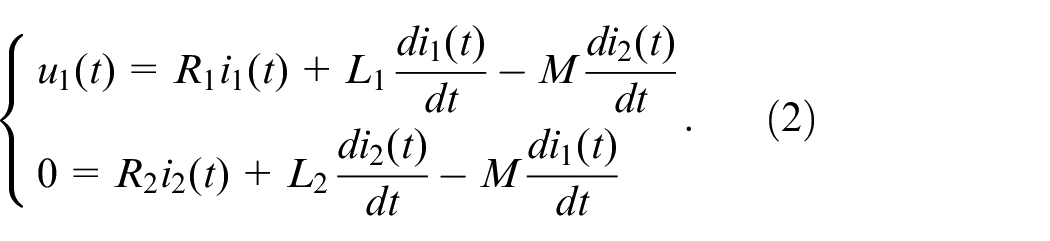
{\begin{matrix} u_{1} (t) = R_{1} i_{1} (t) + L_{1} \frac{d i_{1} (t)}{dt} - M \frac{d i_{2} (t)}{dt} \\ 0 = R_{2} i_{2} (t) + L_{2} \frac{d i_{2} (t)}{dt} - M \frac{d i_{1} (t)}{dt} \end{matrix} .

(2)

Upon applying Laplace transform to both sides of equation (2) and performing some simple algebraic transformations, the relationship between the current and the applied voltage in the primary circuit is obtained

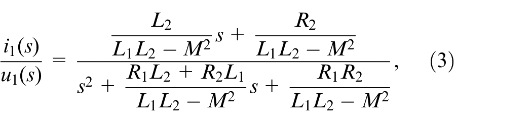
\begin{matrix} \frac{i_{1} (s)}{u_{1} (s)} = \frac{\frac{L_{2}}{L_{1} L_{2} - M^{2}} s + \frac{R_{2}}{L_{1} L_{2} - M^{2}}}{s^{2} + \frac{R_{1} L_{2} + R_{2} L_{1}}{L_{1} L_{2} - M^{2}} s + \frac{R_{1} R_{2}}{L_{1} L_{2} - M^{2}}}, \end{matrix}

(3)

where s is the Laplace operator.

Given that the current $i_{1} (s)$ is used as the probe output, then equation (3) represents the transfer function of the PECT system at the probe terminal, namely

G (s) = \frac{i_{1} (s)}{u_{1} (s)} = \frac{b_{1} s + b_{2}}{s^{2} + a_{1} s + a_{2}},

(4)

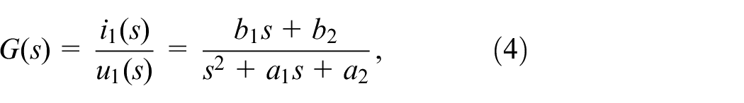
where the parameters a₁, a₂, b₁ and b₂ are given by

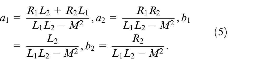
\begin{matrix} a_{1} = \frac{R_{1} L_{2} + R_{2} L_{1}}{L_{1} L_{2} - M^{2}}, a_{2} = \frac{R_{1} R_{2}}{L_{1} L_{2} - M^{2}}, b_{1} \\ = \frac{L_{2}}{L_{1} L_{2} - M^{2}}, b_{2} = \frac{R_{2}}{L_{1} L_{2} - M^{2}} . \end{matrix}

(5)

Equation (4) indicates that the PECT system can be described by a second order system. The corresponding parameters in equation (5), which are related to R₁, R₂, L₁, L₂ and M, will also carry dynamic information of the inspected specimen.

It should be mentioned that there are usually two types of probes, viz., the absolute probe and the transmitter-receiver (TR) probe, used in practical PECT systems.^22,23 The absolute probe only has a single coil and thus matches with the above equivalent circuit model and the corresponding transfer function. However, for the TR probe which utilizes one coil to transmit the primary magnetic field and the other coil to receive the secondary magnetic field, the presented model need to be modified to take into account the coupling between the transmitter and the receiver.

System identification

System identification is a widely used technique in control engineering to characterize an unknown system when its inputs and outputs are given or can be measured. The essence of system identification is to select a model structure that fits the observed input-output data according to a given criterion.^24–26

Equation (4) gives the model structure but the parameters a_i and b_i (i = 1, 2) are undetermined. System identification is used to estimate these parameters. To guarantee the accuracy of estimation, the spectrum of the input signal must be sufficient to cover the spectrum of the system. Although a white noise is such a signal, it is not easy to implement in actual digital systems. A pseudo-random binary sequence (PRBS) is both a practical choice and also can provide rich input in the case of linear system identification.²⁶ There are many types of PRBSs and the most popular type is the m-sequence (maximum length sequence). It is a positive-negative bipolar signal which can be generated using linear feedback shift registers (LFSB) that implement linear recursion. An n-stage LFSB is capable of producing an m-sequence with a period of 2ⁿ−1 and signal levels +1 and −1.

It is a consensus that the advantages of PECT over traditional ECT stems from its square-wave excitation which provides rich frequency components. However, a periodic square wave has a discrete spectrum and its amplitude descends as the frequency component gets higher. Figure 2(a) and (b) gives such an example, a 10 Hz square wave of 10 periods and its frequency spectrum obtained by FFT. It is evident that the amplitude of harmonic component decays fast with the increase of frequency. The m-sequence waveform seems like the combination of square waves of different frequencies, but actually exhibits good randomness within one period. Figure 2(c) shows a 10-order m-sequence signal of 10 periods. For clarity, only the first period waveform is displayed. Figure 2(d) plots the corresponding frequency spectrum. It comprises a main lobe and several side lobes, and the main lobe covers a wide range of low frequency components. In contrast to Figure 2(b), from 0 to 500 Hz the amplitude has a continuous distribution and attenuates much slower. This feature makes the m-sequence more suitable than the square wave as the input signal for identification of a PECT system.

Figure 2.

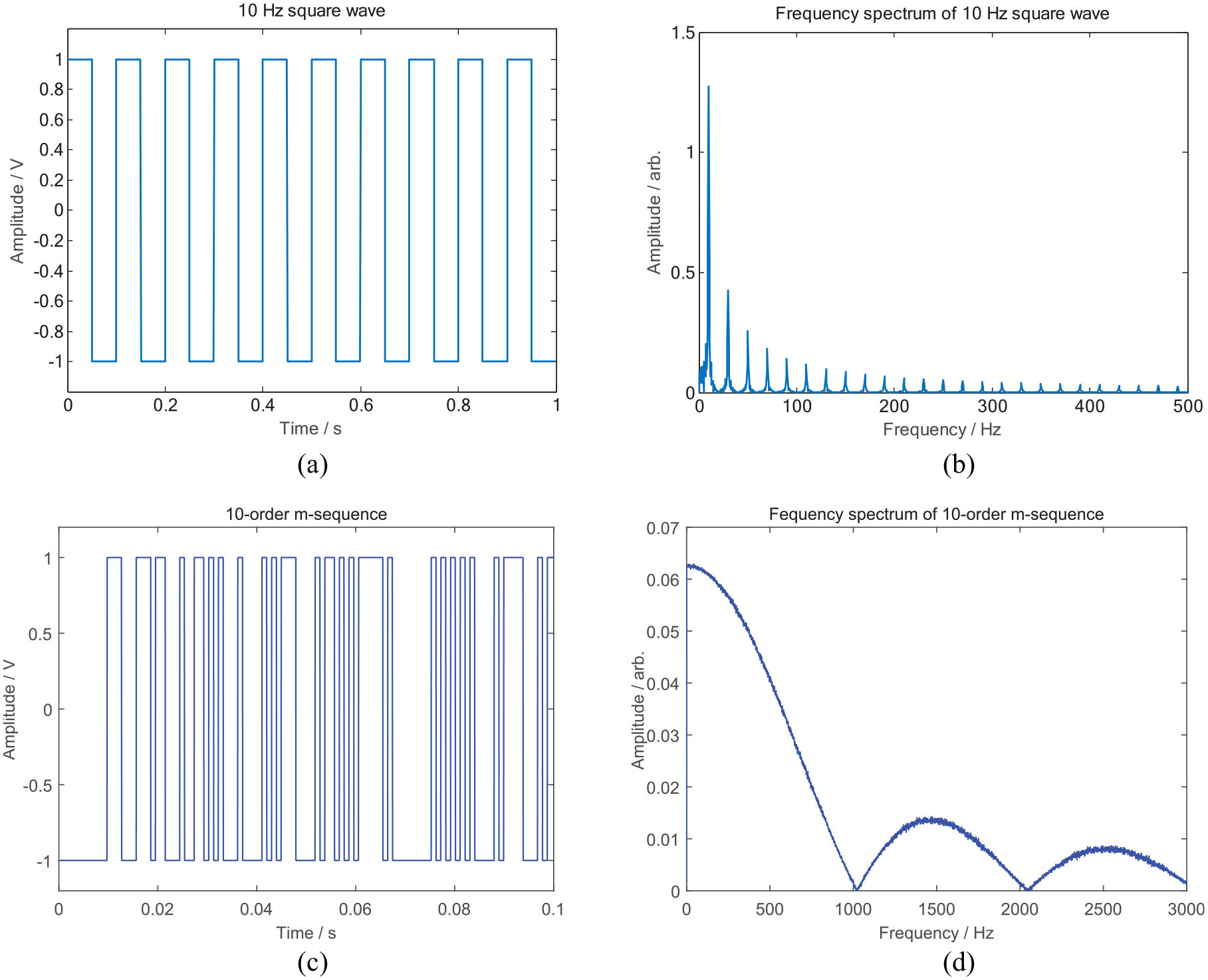
Comparison of waveforms and spectrums of the square wave and the m-sequence: (a) a 10 Hz square wave of 10 periods, (b) the amplitude spectrum of square wave, (c) a 10-order m-sequence, and (d) the amplitude spectrum of m-sequence.

Since the input and output data collected in the experiment are discrete in time domain, the transfer function model should also be represented in the discrete-time form, and thus equation (4) is equivalent to²⁷

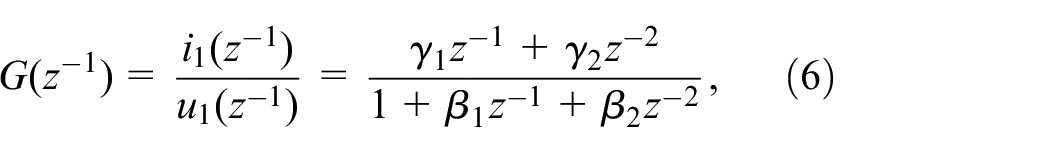
G (z^{- 1}) = \frac{i_{1} (z^{- 1})}{u_{1} (z^{- 1})} = \frac{γ_{1} z^{- 1} + γ_{2} z^{- 2}}{1 + β_{1} z^{- 1} + β_{2} z^{- 2}},

(6)

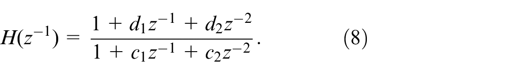
where $z^{- 1} = \frac{2 - T_{s} s}{2 + T_{s} s}$ with T_s denoting the sampling frequency, and the coefficients $β_{i}$ and $γ_{i}$ can be transformed from $a_{i}$ and $b_{i}$ .

Considering the actual output signal always contains noises, then the discrete transfer function model further becomes²⁸

i_{1} (k T_{s}) = G (z^{- 1}) u_{1} (k T_{s}) + H (z^{- 1}) e (k T_{s}),

(7)

where $e (k T_{s})$ represents the white noise and $H (z^{- 1})$ is the noise model which can be expressed as

H (z^{- 1}) = \frac{1 + d_{1} z^{- 1} + d_{2} z^{- 2}}{1 + c_{1} z^{- 1} + c_{2} z^{- 2}} .

(8)

Once the discrete-time model is estimated, it can be converted to the continuous-time model described by equation (4) using the zero-order hold (ZOH).^27,29

With the help of MATLAB System Identification Toolbox,²⁹ the identification process described above can be fast implemented. In the System Identification app, the imported experiment input-output data are processed and examined based on the selected model structure, here the transfer function models. The estimation of model parameters can be done within a short time and the value of best fits which represents the confidence of estimation will also be given.

Calculation of model parameters

Calculation of M

Through the above identification, parameters of a₁, a₂, b₁ and b₂ are determined. There are five variables R₁, L₁, R₂, L₂ and M in equation (5) but only four sub-equations are given. One variable must be calculated in advance to solve equation (5). In fact, we can obtain the value of parameter M using 3D finite element simulation.

The probe coil is a cylindrical multi-turn coreless coil. If the Joule heat is neglected, the energy stored by the coil is equal to the work needed to produce a current through the coil. The formula for this energy is given as

W = \frac{1}{2} L I^{2},

(9)

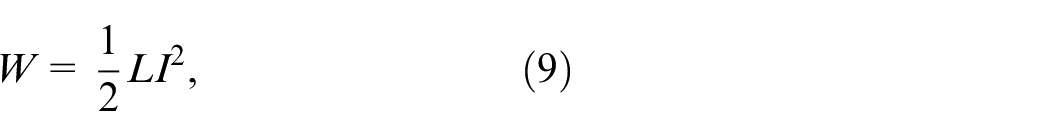
where L is the coil self-inductance and I is the conduction current in the coil.

In large class of materials, there exists a linear constitutive relationship between the magnetic flux density B and the magnetic field intensity H, then the magnetic field stores energy of³⁰

W = \frac{1}{2} \int \int \int H \cdot B d V,

(10)

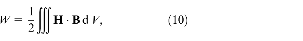
where the integral is evaluated over the entire region where the magnetic field exists.

Combining equations (9) and (10) yields

L = \frac{1}{I^{2}} \int \int \int H \cdot B d V .

(11)

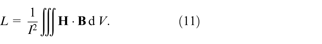
The magnetic flux generated by the probe coil partly penetrates into the specimen while the rest only residents in the air, as the red and black flux lines illustrated in Figure 3. The former part contributes to the formation of mutual inductance M as we stated in preceding modelling. Similar to equation (11), we can write M as

M = \frac{1}{I^{2}} \int \int \int H \cdot B d V',

(12)

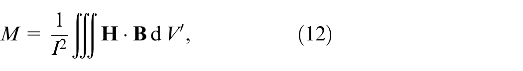
where V’ refers to the region occupied by the magnetic field coupling with the specimen.

Figure 3.

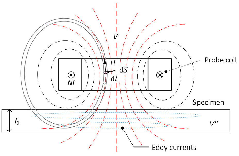
Illustration of magnetic field interaction between probe coil and specimen.

However, it is not practical to factor out V’ from the solution domain in simulation. Since the generated magnetic flux lines are closed, we can assume a unit magnetic path encircling the coil cross section, as shown in Figure 3. Then, dV’ can be written as dSdl and equation (12) becomes $M = \frac{1}{I^{2}} \int \int (\oint H \cdot d l) B d S$ . According to the Ampère’s Law, $\oint H \cdot d l = NI$ with N denoting the number of coil turns. Thus

M = \frac{N}{I} \int \int B d S .

(13)

For a given specimen, the maximum area involved in the probe-to-specimen interaction is the specimen’s upper surface. During 3D simulation, the data of the magnetic flux density B are stored in discrete volumetric elements. In order to accommodate the data extraction, equation (13) is finally modified to

M = \frac{N}{I} \int \int B d S = \frac{N}{I l_{0}} \int \int \int B d S d l = \frac{N}{I l_{0}} \int \int \int B d V ″,

(14)

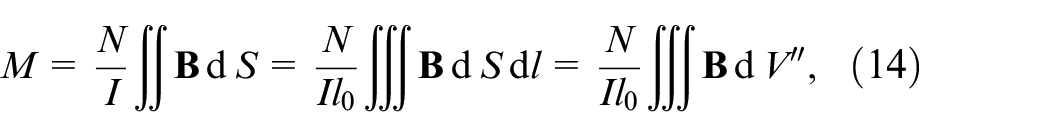
where l₀ is the characteristic thickness of the specimen and V” is the characteristic volume which equals to the product of l₀ and the area of the upper surface. l₀ can be related to the penetration depth of eddy currents, say three times of the standard penetration depth.

Calculation of R_i and L_i

Figure 4 shows the procedure of determining equivalent circuit model parameters R_i and L_i (i = 1, 2). It mainly includes the aforementioned input-output data acquisition, system identification and finite element simulation. The excitation voltage of the PECT probe is a bipolar m-sequence, which is generated by a 16 bit NI PXIe-6368 card and then strengthened by a power amplifier with a gain of K_p. A precise resistor with a resistance of R_s is connected in series with the probe coil and the voltage across it is sampled by a 24-bit NI PXIe-4497 A/D card. Hence, the output current of the probe is obtained by dividing the voltage by the resistance.

Figure 4.

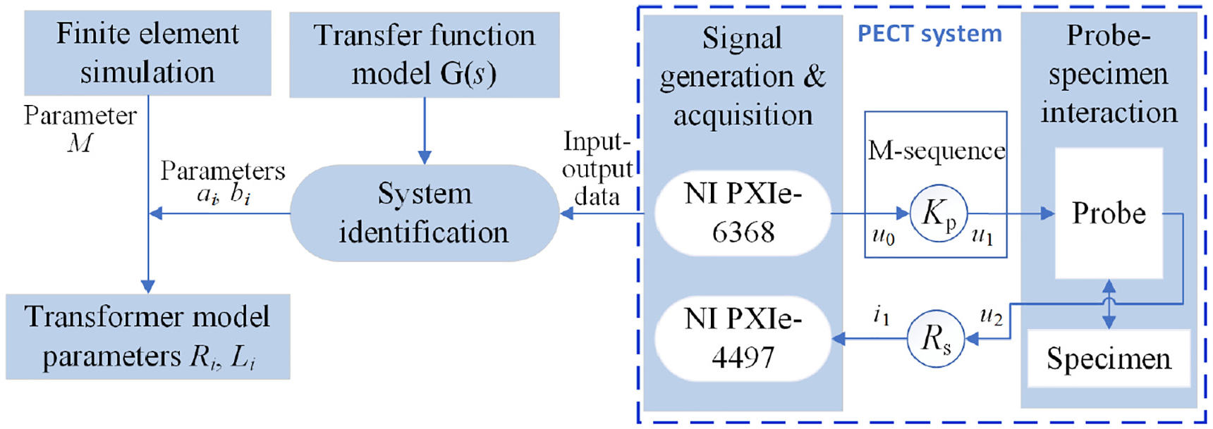
Procedure of obtaining the equivalent circuit model parameters.

Figure 5 shows the waveforms of the probe input and output signals. The input m-sequence has a substantial amount of overshoot and ringing at some rising and falling edges, which might be attributed to the impedance mismatching among instruments during signal transmission.

Figure 5.

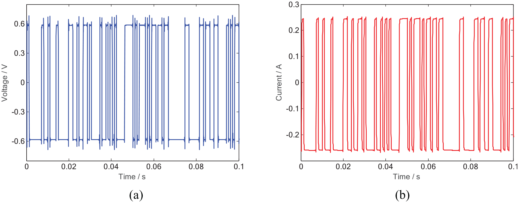
Waveforms of the probe: (a) input and (b) output signals.

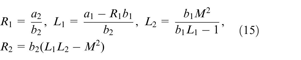
On condition that M, a_i and b_i are obtained using finite element simulation and system identification, from equation (5), the expressions for R_i and L_i can be successively deduced

\begin{matrix} R_{1} = \frac{a_{2}}{b_{2}}, L_{1} = \frac{a_{1} - R_{1} b_{1}}{b_{2}}, L_{2} = \frac{b_{1} M^{2}}{b_{1} L_{1} - 1}, \\ R_{2} = b_{2} (L_{1} L_{2} - M^{2}) \end{matrix}

(15)

Application to defect evaluation

In this section, preliminary PECT experiments are carried out on two defected specimens and the experiment data are processed through the procedure presented in Figure 4. The identified R₂ and L₂ are found to have monotonic correlation with the defect size.

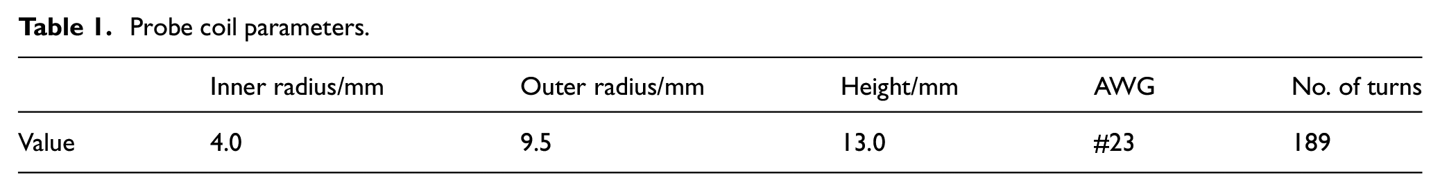
Figure 6 depicts the probe and specimens used in experiments. A coreless cylindrical coil is used as the probe coil and its geometric parameters are listed in Table 1. Two slabs made of aluminium alloy 6061 are used as the specimens. Specimen #1 is 10 mm thick and machined with five through-slots with the same depth of 5 mm but different widths of 2, 4, 6, 8 and 10 mm, labelled by S1 to S5 respectively. Specimen #2 is 16 mm thick and fabricated with five slots with the same width of 2 mm but different depths of 2, 4, 6, 8 and 10 mm, labelled by S’1 to S’5 respectively. The probe coil is excited with an m-sequence signal. The m-sequence length concerns the signal’s interference immunity to white noise. Basically, the longer the sequence is, the weaker is the noise impact. However, a long sequence also means a long measurement period is needed, causing the possibility of signal nonstationarity and discontinuity increasing.³¹ After some initial trials, a 10-order m-sequence with the length of 2¹⁰−1 is selected. The voltage across a 2 Ω resistor connected in series with the probe coil is measured as the output signal. In order to shorten the signal transfer path thus reducing signal distortion, the output is directly sampled by an A/D card without being processed by a preamplifier beforehand.

Figure 6.

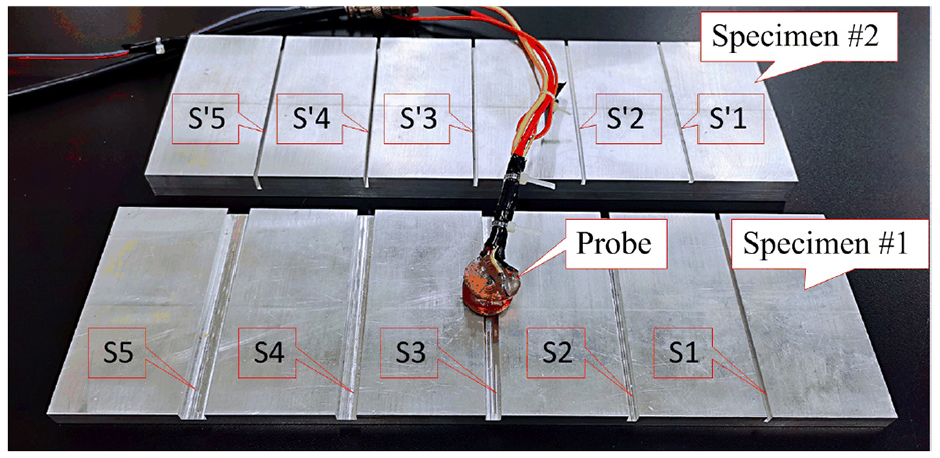
Photo of the probe and specimens.

Table 1.

Probe coil parameters.

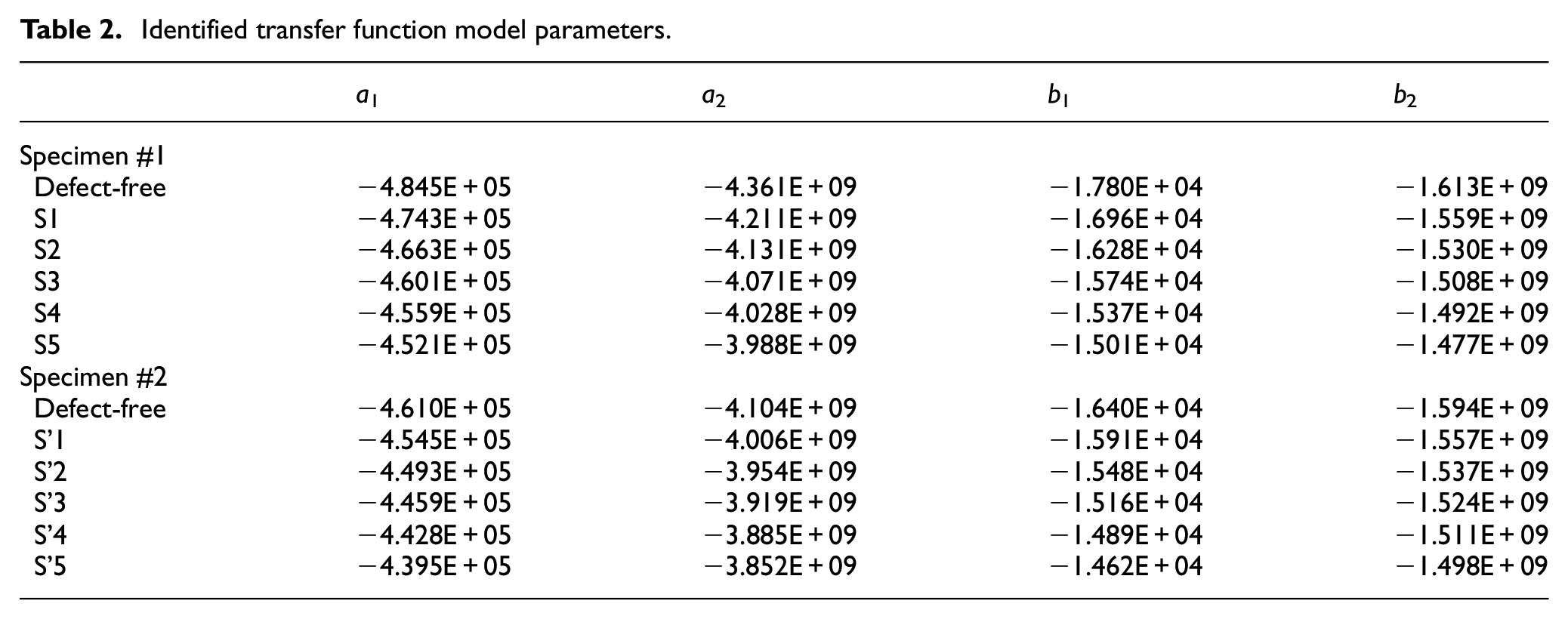
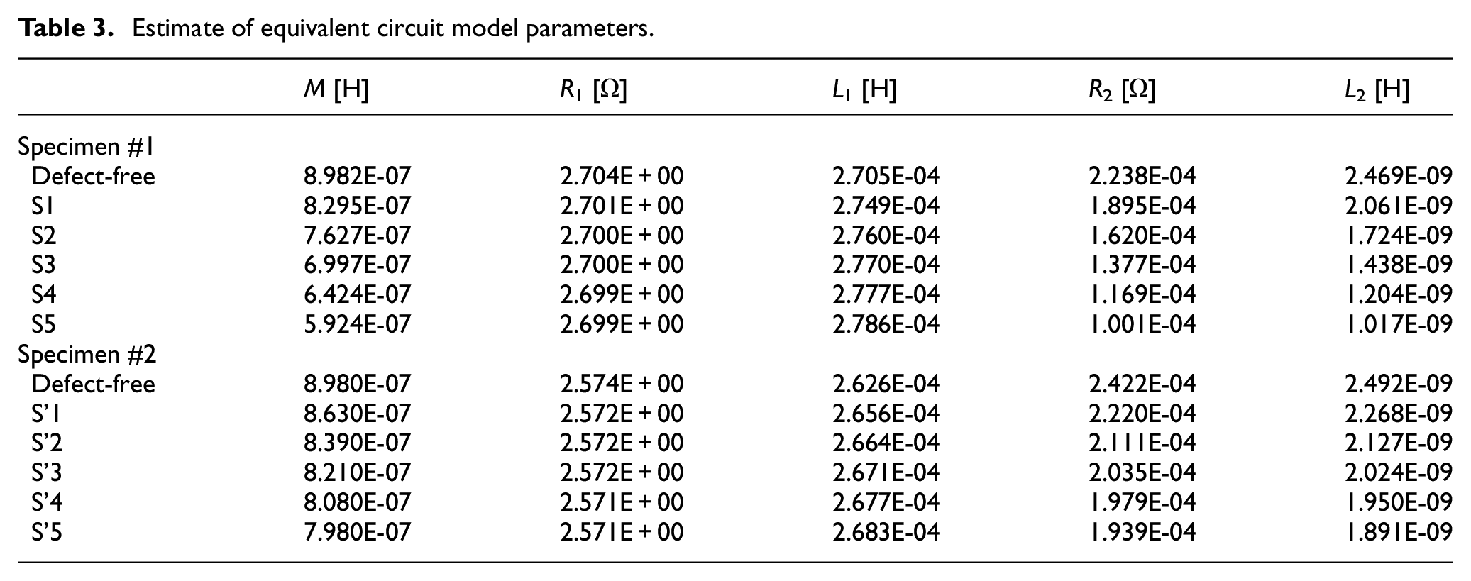
	Inner radius/mm	Outer radius/mm	Height/mm	AWG	No. of turns
Value	4.0	9.5	13.0	#23	189

During experiments, the probe is manually held on the specimen with the coil centre aimed at the slot. The defect-free region of the specimen is also tested as a reference. Table 2 gives the identified transfer function parameters based on acquired experiment data while Table 3 shows the estimate of equivalent circuit model parameters. For a group of input-output data with the duration of 1 s and sampling rate of 100 kS/s, the time consumed in the identification process was about 26.9 s, using a computer equipped with a processor of Intel Xeon E5-2680 v2 and a RAM of 8 GB. Although all the identified a_i and b_i present the same changing trend, diverse variations are observed for estimated R_i and L_i. From the defect-free case to the biggest defect case, R₁ holds almost the same value while L₁ slightly increases. The relatively larger variations are found for R₂ and L₂ which decrease by 55.3% and 58.8%, respectively, for the specimen #1. While for the specimen #2, R₂ and L₂ decrease by 19.9% and 24.1%, respectively. These variation trends are in accordance with the implication of equation (15). As seen in equation (15), only the expressions of R₂ and L₂ contain M, which indicates that these two parameters are tightly related to the specimen status. Hence, R₂ and L₂ can be selected as the features to evaluate the defect.

Table 2.

Identified transfer function model parameters.

	a ₁	a ₂	b ₁	b ₂
Specimen #1
Defect-free	−4.845E+05	−4.361E+09	−1.780E+04	−1.613E+09
S1	−4.743E+05	−4.211E+09	−1.696E+04	−1.559E+09
S2	−4.663E+05	−4.131E+09	−1.628E+04	−1.530E+09
S3	−4.601E+05	−4.071E+09	−1.574E+04	−1.508E+09
S4	−4.559E+05	−4.028E+09	−1.537E+04	−1.492E+09
S5	−4.521E+05	−3.988E+09	−1.501E+04	−1.477E+09
Specimen #2
Defect-free	−4.610E+05	−4.104E+09	−1.640E+04	−1.594E+09
S’1	−4.545E+05	−4.006E+09	−1.591E+04	−1.557E+09
S’2	−4.493E+05	−3.954E+09	−1.548E+04	−1.537E+09
S’3	−4.459E+05	−3.919E+09	−1.516E+04	−1.524E+09
S’4	−4.428E+05	−3.885E+09	−1.489E+04	−1.511E+09
S’5	−4.395E+05	−3.852E+09	−1.462E+04	−1.498E+09

Table 3.

Estimate of equivalent circuit model parameters.

	M [H]	R ₁ [Ω]	L ₁ [H]	R ₂ [Ω]	L ₂ [H]
Specimen #1
Defect-free	8.982E-07	2.704E+00	2.705E-04	2.238E-04	2.469E-09
S1	8.295E-07	2.701E+00	2.749E-04	1.895E-04	2.061E-09
S2	7.627E-07	2.700E+00	2.760E-04	1.620E-04	1.724E-09
S3	6.997E-07	2.700E+00	2.770E-04	1.377E-04	1.438E-09
S4	6.424E-07	2.699E+00	2.777E-04	1.169E-04	1.204E-09
S5	5.924E-07	2.699E+00	2.786E-04	1.001E-04	1.017E-09
Specimen #2
Defect-free	8.980E-07	2.574E+00	2.626E-04	2.422E-04	2.492E-09
S’1	8.630E-07	2.572E+00	2.656E-04	2.220E-04	2.268E-09
S’2	8.390E-07	2.572E+00	2.664E-04	2.111E-04	2.127E-09
S’3	8.210E-07	2.572E+00	2.671E-04	2.035E-04	2.024E-09
S’4	8.080E-07	2.571E+00	2.677E-04	1.979E-04	1.950E-09
S’5	7.980E-07	2.571E+00	2.683E-04	1.939E-04	1.891E-09

Figures 7 and 8 plot the variations of R₂ and L₂ whose values are normalized to the value of the defect-free case for the specimen #1 and specimen #2, respectively. It can be seen that both parameters decrease monotonically with the slot size (width or depth). The L₂ curve is steeper than the R₂ curve, suggesting L₂ a more sensitive feature for defect evaluation. However, as shown in Table 3, the order of magnitude of R₂ is much larger than that of L₂, which means R₂ might be more robust to interferences in practical application. In addition, it can be concluded from the two figures that R₂ and L₂ are more sensitive to the defect width than the defect depth. The possible ways to increase the depth sensitivity may include using a smaller diameter probe coil and a high sensitive receiver element. More studies regarding detailed characteristics of the two features in various testing conditions need to be further conducted.

Figure 7.

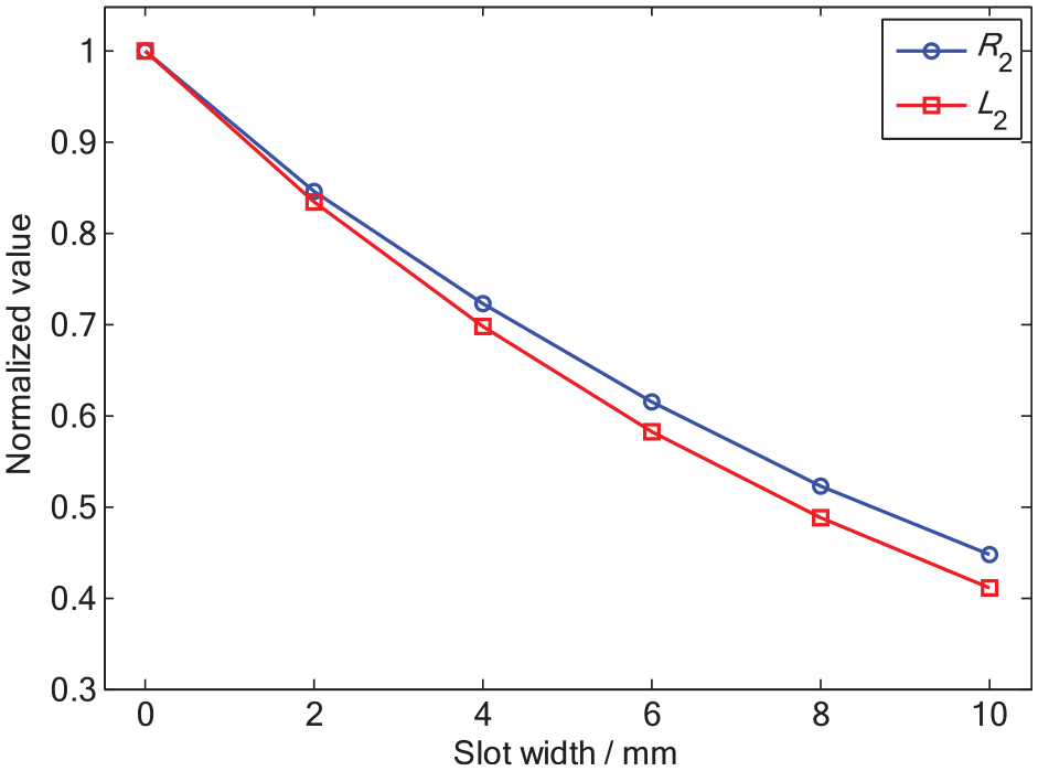
Plots of normalized R₂ and L₂ values against slot width of specimen #1_..

Figure 8.

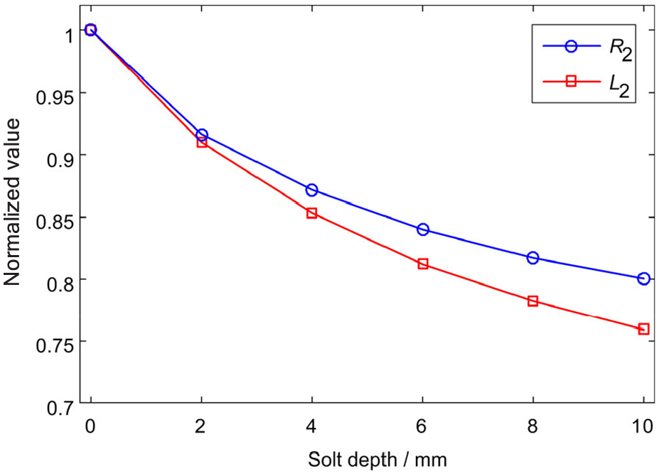
Plots of normalized R₂ and L₂ values against slot depth of specimen #2_..

Conclusion

PECT equivalent circuit model has relatively simple mathematical expressions but usually serves as a tool in textbooks for qualitative interpretation of the PECT principle. This paper concerns the estimate of equivalent circuit model parameters and touches on the application of model parameters in aspect of defect evaluation. By regarding the probe-to-specimen interaction as a mutual inductance, the probe and specimen are respectively modelled as the primary and secondary windings of a transformer. The transformer circuit equations are tackled from the perspective of system analysis and the transfer function is formulated in Laplace domain. To determine the transfer function parameters, system identification approach was applied. The m-sequence, which shows good randomness within one period and uniform spectrum profile in a wide range of frequency, is used as the probe input signal. A set of experiment input-output data are acquired by performing experiments on two aluminium alloy 6061 slabs, one of which is machined with five width-varied slots and the other is machined with five depth-varied slots. The transfer function model parameters are identified using the MATLAB System Identification Toolbox.

The mutual inductance between the probe coil and the specimen is calculated using a novel method based on the magnetic field energy allocated to the probe-to-specimen coupling. Other equivalent circuit parameters including resistance and self-inductance are estimated based on the identified transfer function parameters. It is found that the resistance and self-inductance of the secondary windings decrease greatly and monotonically as the slot size (width or depth) increases. The self-inductance is more sensitive to the variation of slot size than the resistance. Both of them have the potential to serve as the signal feature for defect evaluation.

Compared with conventional PECT signal features such as peak value, time to peak and time-to-zero crossing, the features extracted from estimated parameters are thought to be more robust to the effects of noise and measurement errors because most system identification methods are capable of dealing with noise and measurement errors. However, the parameter identification also introduces an extra step for PECT signal processing, which makes the detection speed slow down in the practical application. Thus, the future work will focus on optimizing the computation speed using advanced algorithms for the identification of transfer function parameters.

Footnotes

Declaration of conflicting interests

The author(s) declared no potential conflicts of interest with respect to the research, authorship, and/or publication of this article.

Funding

The author(s) disclosed receipt of the following financial support for the research, authorship, and/or publication of this article: This work was supported by National Natural Science Foundation of China under Grant No. 51505406.

ORCID iD

Zhiyuan Xu

References

Xie

Zhang

Zhao

, et al. Features extraction and discussion in a novel frequency-band-selecting pulsed eddy current testing method for the detection of a certain depth range of defects. NDT & E Int 2020, 111: 102211.

Waidelich

. Coating thickness measurements using pulsed eddy currents. In: Proceedings of the national electronics conference, Chicago, IL, 4–6 October 1954, vol. 10, pp.500–507.

Wang

. Thickness and conductivity measurement of multilayered electricity-conducting coating by pulsed eddy current technique: experimental investigation. IEEE Trans Instrum Meas 2019; 68(9): 3166–3172.

Wang

Fan

Cao

, et al. Measurement of coating thickness using lift-off point of intersection features from pulsed eddy current signals. NDT&E Int 2020, 116: 102333.

Zhu

. Measurement of accumulated height of exfoliated oxide scales in austenitic boiler tubes using pulsed eddy current testing. Russ J Nondestr Test 2020; 56(4): 350–360.

Eddy

Underhill

Morelli

, et al. Pulsed eddy current response to general corrosion in concrete rebar. J Nondestruct Eval Diagn Progn Eng Syst 2020, 3(4): 044501.

AbdAlla

Faraj

Samsuri

, et al. Challenges in improving the performance of Eddy current testing: review. Meas Control 2019; 52(1–2): 46–64.

Liu

, et al. Pulsed eddy current data analysis for the characterization of the second-layer discontinuities. J Nondestr Eval 2018; 38: 7.

Mardaninejad

Safizadeh

. Gas pipeline corrosion mapping through coating using pulsed eddy current technique. Russ J Nondestr Test 2019; 55(11): 858–867.

10.

, et al. Assessment of wall thinning in insulated ferromagnetic pipes using the time-to-peak of differential pulsed eddy-current testing signals. NDT & E Int 2012; 51: 24–29.

11.

Dodd

Deeds

. Analytical solutions to Eddy-current probe-coil problems. J Appl Phys 1968; 39(6): 2829–2838.

12.

Sun

Shi

Zhang

. Time-domain modeling analysis of pulsed eddy current testing on ferromagnetic casing. Rev Sci Instrum 2020; 91: 94702.

13.

Qing

Xin-Jun

. Analytical modeling for the plate with a flat-bottom hole based on the reflection and transmission theory in pulsed eddy current testing. Acta Phys Sin 2017; 66(3): 38102.

14.

Terekhin

Slavinskaya

. Evaluating specific electrical conductivity of two-layered nonmagnetic objects by pulsed eddy-current method. Russ J Nondestr Test 2019; 55(4): 286–292.

15.

Lefebvre

JHV

Mandache

Letarte

. Pulsed eddy current empirical modeling. In: Proceeding of the Vth international workshop, advances in signal processing for non destructive evaluation of materials, Quebec, Canada, 2–4 August 2005, pp.69–74.

16.

Vyroubal

. Impedance of the Eddy-current displacement probe: the transformer model. IEEE Trans InstrumMeas 2004, 53(2): 384–391.

17.

Tondo

Porto

Villalobos

, et al. Eddy current probe identification and analysis. IEEE Trans InstrumMeas 2017; 66(8): 2166–2173.

18.

Dadić

Vasić

Bilas

. A system identification approach to the modelling of pulsed Eddy-current systems. NDT & E Int 2005; 38(2): 107–111.

19.

Lang

Agurto

Tian

, et al. A system identification based approach for pulsed Eddy current non-destructive evaluation. Meas Sci Technol 2007; 18(7): 2083–2091.

20.

Lee

Johnson

Nakagawa

. Development of a pulsed eddy current system and its characterization. In: AIP conference proceedings, Portland, OR, 21 March 2007, pp.354–361. American Institute of Physics.

21.

Nakagawa

Lee

, et al. Pulsed eddy current system characterization and benchmark waveforms. In: AIP conference proceedings, Golden, CO, 10 March 2008, pp.407–413. American Institute of Physics.

22.

Wang

Deng

. Rotating focused field Eddy-current sensing for arbitrary orientation defects detection in carbon steel. Sensors 2020; 20(8): 2345.

23.

Zhang

. Study on the shielding effect of claddings with transmitter–receiver sensor in pulsed Eddy current testing. J Nondestr Eval 2019; 38(4): 99–110.

24.

Ljung

. System identification: theory for the user. 2nd ed. Upper Saddle River, NJ: Prentice-Hall, 1999.

25.

Mwaniki

Vermeulen

. Characterization and application of a pseudorandom impulse sequence for parameter estimation applications. IEEE Trans Instrum Meas 2020; 69(6): 3917–3927.

26.

Roinila

Abdollahi

Santi

. Frequency-domain identification based on pseudorandom sequences in analysis and control of DC power distribution systems: a review. IEEE Trans Power Electron 2021; 36(4): 3744–3756.

27.

Oppenheim

. Discrete time signal processing. 3rd ed. Upper Saddle River, NJ: Pearson Higher Education Inc., 2010, p.504.

28.

Lomov

Fedoseev

. Comparison of parameter identification methods for linear dynamic systems under mixed noise. J Math Sci 2021; 253(3): 407–418.

29.

Ljung

. System identification toolbox: user’s guide. Natick, MA: MathWorks Incorporated, 1995.

30.

Jackson

. Classical electrodynamics. 3rd ed. New York, NY: Wiley, 1999.

31.

. Pseudo-random signal and correlation identification (in Chinese). Beijing: Science Press, 1987.

Parameter identification of pulsed eddy current testing equivalent circuit model and its application to defect evaluation

Abstract

Keywords

Introduction

Equivalent circuit modelling

System identification

Calculation of model parameters

Calculation of M

Calculation of Ri and Li

Application to defect evaluation

Conclusion

Footnotes

Declaration of conflicting interests

Funding

ORCID iD

References

Calculation of R_i and L_i