Sage Journals: Discover world-class research

Abstract

An implementation of a two-stage piece-wise linearization method for reduction of the thermocouple approximation error is presented in the paper. First, the whole thermocouple measurement chain of a transducer is described, and possible error is analysed to define the required level of accuracy for linearization of the transfer characteristics. Evaluation of linearization functions and analysis of approximation errors are performed by the virtual instrumentation software package LabVIEW. The method is appropriate for thermocouples and other sensors where nonlinearity varies a lot over the range of input values. The basic principle of this method is to first transform the abscissa of the transfer function by a linear segment look-up table in such a way that significantly nonlinear parts of the input range are expanded before a standard piece-wise linearization. In this way, applying equal-segment linearization two times has a similar effect to non-equal-segment linearization. For a given examples of the thermocouple transfer functions, the suggested method provides significantly better reduction of the approximation error, than the standard segment linearization, with equal memory consumption for look-up tables. The simple software implementation of this two-stage linearization method allows it to be applied in low calculation power microcontroller measurement transducers, as a replacement of the standard piece-wise linear approximation method.

Keywords

Two-stage linear approximation thermocouple transfer curve approximation error reduction virtual instrumentation

Introduction

The nonlinear transfer curve of the sensors in the intelligent measuring transducers can be compensated by one of the numerous hardware and software-based methods. Some of the most common software methods for transfer curve linearization are: standard piece-wise linearization, approximation with a polynomial in the entire range, or divided into the segments of the input value, including spline, rational functions approximation, and approximation by the neural networks.

The polynomial approximation is a standard method for thermocouple transfer curve. Equations suitable for linearization of each type of thermocouple are given by NIST and BIPM official documents in the form of polynomial approximations of eighth order and above, for more (up to 5) linearization segments, with a very small approximation error.^1,2 Allowed thermocouple errors, obtained in the production process and caused by sensor ageing, are significantly larger,³ typically over 1°C. That enables low-order polynomial functions⁴ or low-order spline functions⁵ to be successfully used for sensor linearization. In the paper⁴ reduction of the polynomial order for thermocouples of type J and T was achieved by choosing to work in a narrow operating range. An iterative procedure for the addition of non-equidistant B-spline nodes for interpolation, based on the third derivative of the function is considered in the paper.⁵ They achieved an error of 0.2°C with 33 free points for a type S thermocouple, at a full range up to 1400°C, using a B-spline curve of degree 4.

In the paper⁶ a progressive polynomial calibration method is proposed, where the polynomial is determined directly from the calibration measuring points, which is especially suitable if the transfer characteristic is not known. All imperfections of the measurement chain are then compensated for in the same procedure.

Artificial Neural Networks (ANN) are proposed as a linearization method in several papers. In the paper⁷ linearization of several types of thermocouples was performed. For E type thermocouple, in the range from −200°C to 1000°C, an error of 0.5% was achieved, that is, 5°C, which is not a satisfying result. In the paper⁸ an ANN was applied to the linearization of NTC sensors, showing an advantage for auto-calibration with a smaller number of reference points compared to the polynomial and piece-wise methods. ANN methods are suitable to include the correction of the measurement chain imperfections, but also influential quantities, such as the temperature of the cold junction.⁹

Overall required memory and calculation overhead are very important aspects when selecting optimal linearization methods for specific applications.

Calculation of the optimal linearization coefficients, based on a known function or calibration points, can usually be performed within a personal computer. With the use of the computer’s vast resources, the application of complex algorithms is not constrained. On the other hand, measurement transducer usually has significantly weaker resources in the form of memory and processing power, so in this case, it is very important to use a linearization method in which the calculation of a response in the measurement transducer is not highly demanding in the terms of required memory and processor power.^10–12 A small number of microprocessor cycles required for the calculation is more important when a device supports a bigger number of input channels or direct multiplexing of a number of sensors at the input stage.

If linearization error of less than 1% is required, but transfer function is significantly nonlinear, the number of used segments of the standard piece-wise method must be increased significantly. If the polynomial approximation is used, a higher degree of the polynomial is required.⁴

In the paper¹⁰ interpolation in low-power microcontrollers is clearly presented, starting from the complete LUT to a piece-wise interpolation, by selecting m higher bits for the index in the table of samples (additional division is avoided). The analysis is given on the example of an NTC sensor.

In many applications, it can be useful to perform calculations with integers only, which is more compatible with linear segment approximation. Implementation of arithmetic for floating-point data format inside microcontrollers can spend about 1 Kbyte of program memory, big enough for up to 500 segments of the linearization table in integer data type.¹² In addition to faster calculations, this makes piece-wise linearization in integer data format more applicable than a polynomial approximation, and very appropriate for implementation in microcontroller transducer for different sensor types. It is also suitable for two-dimensional segment (surface) linearization, when the final result depends on two variables, that is, if, in addition to the main signal, ambient temperature or pressure cross-sensitivity exist, which should be included in calculations.

The piece-wise approximation of biological signals (ECG) in the form of connected segments is shown in the paper,¹³ taking into account the memory consumption, as well as that the response speed of the method.

Many of published papers combine the presentation of linearization methods with a practical implementation of the transducer measuring chain electronics.^6,7,9,11,14

Papers^11,15 give a good comparative analysis of the application of a wider group of methods including fuzzy logic, in addition to the already mentioned. The paper¹¹ specifically compares the methods on the example of a given characteristic of an optical distance sensor and using a low-power microcontroller, showing that ANN and fuzzy methods are not appropriate in this case. Then, the advantage of the piece-wise methods is demonstrated, especially when the gain of the measurement chain is changed by a built-in Programmable Gain Amplifier (PGA) circuit. This is a type of two-step linearization, but also a hardware-dependent approach.

The paper¹⁵ gives a very detailed comparative summary of sensor characteristics linearization, including various sensors and methods, starting from hardware methods to software methods, emphasizing the advantage of software methods, especially for thermocouples. The hardware implementation of the piece-wise method is also considered here, as well as in the papers.^16,17 Of the software methods piece-wise, polynomial, ANN, and fuzzy methods are highlighted.

It is very difficult to achieve an adequate comparison of the methods, as the accuracy of the approximation depends a lot on the observed transfer characteristic, but also on the memory spent on coefficients, and the required speed of response.

Thermocouple input stage

Thermocouples are frequently used as temperature sensors, due to their fast response, robust construction, and temperature range from −270°C to 2500°C, which is wide in comparison to other, typically resistive and semiconductor-based temperature sensors.^18,19 In addition to the nonlinearity of the transfer characteristic, the most significant problem with the practical application of thermocouples is the influence of the cold junction temperature.⁴ Two metal wires with different thermoelectric characteristics are joined together at one side, and this side is exposed to different, and usually much higher temperature than the other side. The voltage difference between wires at the open end will depend on wire materials and temperatures at both ends. Table with the thermoelectric voltage of standard thermocouples is given assuming that the open wire side has a temperature of 0°C. Outside the furnace, that is, a zone with a very high temperature, thermocouple wires can be extended with a less expensive compensating cable to the position of the electronics. In order to be able to measure the temperature at the junction, the temperature at the open end must be known. That end is usually referred to as the “cold junction”.^9,20 For solving the problem of cold junction temperature compensation in practical applications an additional temperature sensor with usually better accuracy, but with a much smaller temperature range is used, for example, NTC or Pt100 resistant type sensor, or even a semiconductor type sensor like TMP275, connected via the I2C digital interface.

One specific example of a practical implementation of the thermocouple signal chain with a cold junction temperature sensor and additional electronics is presented in Figure 1. Each segment in the presented block diagram of a thermocouple signal chain will affect the measurement accuracy and must be carefully selected to minimize the error. In the given schematic, one can see the polarization of the input terminal, with resistors R₁, R₂, and R₃. In the case of thermocouple interruption, this set of resistors leads the signal into saturation. Components R₆, D₁, and R₄ protect from input high voltages. In addition, many elements (L₁, L₂, C₆, R₆, C₅, R₄, C₇, R₅, C_8, as well as C_13, and sigma-delta ADC) enable filtration of input interferences. Low-pass filtering is effective because the required conversion rate for such applications is usually low, for example, few samples per second, because temperature typically does not change very quickly. An amplifier is required due to a low thermocouple output, which is in the millivolts range. If a universal input circuit is used for a different type of thermocouple, mentioned in the chapter below, input range should cover a wider range, that is, from −8.83 mV up to 76.4 mV. For very low-level output voltage signals, an amplifier with a small offset voltage temperature coefficient must be used, for example, amplifier OP177, with an offset voltage temperature coefficient value of 0.3 µV/°C.

Figure 1.

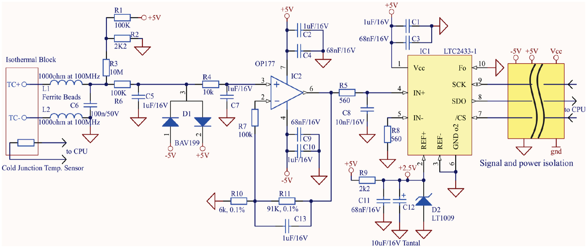
Block scheme of the thermocouple transducer practical implementation.

It can be calculated that the average sensitivity of type B thermocouples is about 7.6 µV/°C, which implies that components with good stability, small temperature coefficients, and final calibration of the whole measurement chain are strongly required. Even in that case, if the operating temperature of transducer electronics varies by ±20°C, then a temperature measurement error of ±1°C can be expected.

Considering a very small input signal value of the thermocouple, if a measurement device has several input and output signals, electrical insulation is almost certainly necessary, in order to eliminate errors caused by ground mass differences. This will prevent dangerous common voltage signals exceeding the input limits of the amplifier. Electrical insulation provides excellent CMRR value (“Common-mode rejection ratio”), especially for low frequency signals, from 100 dB to 140 dB. This enables proper implementations with single-ended configurations of the input amplifier, to have easier filtering, voltage limiting, and implementation of the input saturation circuit for the case of the thermocouple breaking. The Sigma-delta ADC with 16-bits of resolution chosen in the circuit provides notch filtering for 50 Hz/60 Hz noise frequency with the rectification of at least 87 dB, in addition.

The implemented ADC circuit allows a negative voltage of about 300 mV, which is sufficient to cover the negative segment of the thermocouple characteristics, even with required signal amplification of A = 16.2, calculated based on the positive ADC input range of 1250 mV. This input range is defined by reference voltage of U_ref = +2.5 V and ADC range of ±U_ref/2.

Any error in the cold junction measurement will reflect on the calculation of the hot junction temperature value. The on-board temperature sensor needs to be located very close to the input terminals, if possible in the thermostatic chamber with the connector. A typical procedure for software-based linearization of the thermocouple transfer characteristic includes conversion of the cold junction temperature, T_0, to voltage U_0, using the direct function relation between voltage and temperature U₀ = f(T₀). In the next step, the obtained voltage value U₀ needs to be added to the thermocouple output voltage U_T, then inverse function converts the voltage to the measurement temperature according to the formula $T = f^{- 1} (U_{T} + U_{0})$ .^9,20 Due to the nonlinearity of the thermocouple characteristic, adding the cold junction temperature directly to the inverse function of the thermocouple voltage is not correct, as the required $T = f^{- 1} (U_{T} + f (T_{0}))$ is not equal to $T = f^{- 1} (U_{T}) + T_{0}$ .

The block diagram of the data flow algorithm in the measurement transducer, suitable for measurement with various types of thermocouples, is shown in Figure 2. The relation between the results of ADC conversion and the input voltage is the same for all thermocouple types. Usually, in the production of a transducer, it is necessary to change coefficients a_d and b_d, within the calibration procedure. After that, the voltage from the thermocouple should be increased for the voltage obtained from the cold junction sensor. To simplify the linearization method for various types of thermocouples, and to reduce the errors in integer calculations, the signal is then scaled to cover a maximum range of used unsigned int16 variables, from 0 to 65535, for the boundaries of the voltage range for selected the TC type, and the temperature measurement range.

Figure 2.

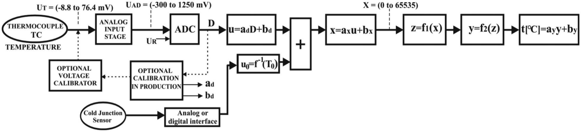
Data flow inside a thermocouple measurement transducer.

The next stage is taking the inverse function of the particular thermocouple. In the given block diagram, this inverse function is decomposed into functions f₁ and f₂, according to the proposed two-stage linearization method. Finally, the calculated temperature integer value in the range from 0 to 65535 can be converted into the final result of temperature measurement in fixed-point arithmetic, by coefficients a_y and b_y (also different for each type of thermocouple), to reach a temperature in the form of yyyy.y [°C]. Thus, with decimal point equal to 1, the resolution will be 0.1°C, still an integer value, but in the signed int16 range.

Introduction of the two-stage linear approximation method applied to standard thermocouples

Thermocouple transfer characteristics are in some parts significantly nonlinear. The linearization method defined by NIST considers the division of the entire measurement range in several unequal segments, so the determination of the specific segment in which the current measurement point is located must be performed in a loop. The main goal of using a two-stage linear segment approximation method, first time proposed in previously published papers,^12,21 is to perform all calculations in integer arithmetic, and also to avoid runtime determination of which of the non-equal segments the input value belongs to.

A non-linear transfer characteristic can be approximated by multiple linear segments, where it is usually required that the segments are connected, as the approximate function should be continuous. One way to define each of the segments is to use the least square deviation method, starting from an array of points from the original function¹² or performed measurements, if the function is unknown. Then, to ensure that the approximated function is continual, segments are joined together by finding boundary ordinate values as the mean value of segments ordinates.

Piece-wise linearization is mostly implemented with equal abscissa segment size. To reduce the error of approximation, increasing the number of segments is required in the areas where the transfer characteristic is strongly nonlinear, usually in a smaller part of the whole characteristic. That leads to non-equal segment sizes. If segments are equal, the response of the linearization algorithm will be fast in finding the index of the current segment and position of points inside, by integer division of input abscissa, that is, x value with the size of the segment. If the number of the segment is given as the power of 2, it is possible to achieve an even faster response, by replacing division with the right bit shifting of the current x value. For example, if the number of segments is 32, right shifting by 5 bits is required to find the rest of x value inside the segment, while those 5 most significant bits represent the current segment number.

Different segment sizes cause the linearization method to be slow, as determining the index of the current segment is performed by comparison of the input variable with a whole table of segment borders in a loop. One way to keep the total number of required segments low, but not to slow down the calculation of the linearization response, due to unequal segments, is the two-stage linearization method proposed in Živanović et al.¹² In that method, parts of the transfer function where the nonlinearity is expressed are determined. Then, the X-axis transformation is performed so that these parts are expanded relative to the rest of the function. This transformation of the X-axis is also performed using a piece-wise linear method. Then, the piece-wise linearization is applied again to the resulting function. The error of this approximation will be lower than without stretching of the non-linear areas. Transformation of the X-axis is realised here in a different manner to the implementation in Živanović et al.¹² because it is based on an iterative process explained in the further text, and not directly based on the range of function’s derivative inside the segments.

The proposed linearization method can be applied to various types of sensors. In the paper, the two-stage linearization method is applied to the standard types of thermocouples: B, E, J, K, R, S, T, and N type are presented. The main requirement for the linearization is that its approximation error is lower than the limit error values defined by NIST and BIPM standards for thermocouples, suitable for practical application and temperature measurements.^1,2 The final error of the linearization in this paper will be calculated as the maximal difference between the ordinate of approximate function and ordinate value of the NIST inverse polynomial function, over the whole range of the voltage for the particular thermocouple. The entire procedure, with the corresponding graphical presentations of the obtained thermocouple characteristics and transfer curves, is performed using software algorithms developed in the LabVIEW programming environment.

The implemented software application enables graphical presentation of the obtained transfer curves for a selected type of thermocouple, presentation of linearized transfer curves, tables with linearization coefficients, and presentation of obtained thermocouple approximation errors. The front panel of the LabVIEW virtual instrument for the presentation of normalized inverse transfer curves obtained for selected an E type of thermocouple is presented in Figure 3. In this diagram, two transfer curves are shown. The first curve, with a white full-line, presents a nominal polynomial approximation of the thermocouple transfer curve - the temperature as a function of the input voltage. This is a monotonically increasing function with a certain level of nonlinearity. This polynomial transfer curve is obtained according to the NIST approximation functions,¹ by scaling the X and Y-axis to the range from 0 to 65535.

Figure 3.

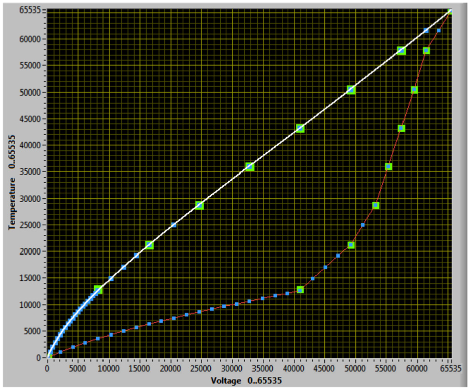
LabVIEW front panel for the presentation of normalized inverse transfer curves for E type of thermocouple – original curve (white) and curve with transformed X-axis (red).

The second, red, transfer curve shows the resulting thermocouple transfer characteristic obtained after the transformation of the X axis. Green dots, shown on both transfer curves, correspond to the initial division of the white (original) transfer curve into eight segments. The red transfer curve, after replacing the X-axis with Z, becomes a function Y = f(Z). This transfer curve is divided into 32 segments, uniformly on the abscissa – the Z axis (shown as blue dots on the red transfer curve). These dots are used as boundaries of the second stage linearization segments. By transferring back the blue dots from the red curve to the white original transfer curve, one can see that practically a segment approximation with unequal division at X-axis will be reached.

Thus, the final linearization of the thermocouple inverse characteristic, and calculation of temperature based on normalized voltage as input, is done according to the relation:

Y = f_{2} (Z) = f_{2} (f_{1} (X)) = f_{T} (X)

(1)

Function Z = f₁(X), which transforms the X-axis on eight equal segments in the range from 0 to 65535 into Z-axis, by the first piece-wise table, is presented at Figure 4, including the arrays of segment input and output values, X and Z.

Figure 4.

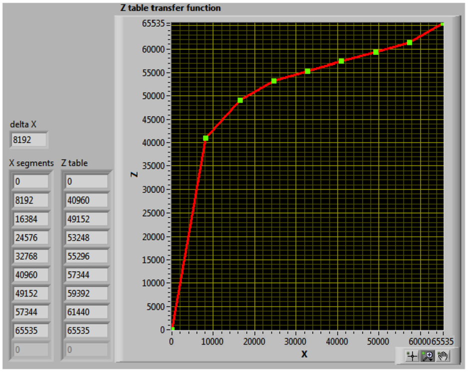
First piece-wise table, which transforms the X-axis on eight equal segments.

LabVIEW block diagram of the software application for the calculation of the segments inside two-stage linearization methods for the thermocouples, including the calculation of the approximation errors, is presented in Figure 5. Iterative calculation of both piece-wise tables is performed in the loop. Input parameters for the operation of this loop are a selection of the number of segments M of the first table, the target value of the maximal allowed overall approximation error (TargetError[°C] in the LabVIEW block diagram), and the maximal allowed number of the segments of the second linearization table (MaxN). In the block diagram, M is left from the While Loop, MaxN and TargetError[°C] are upper right in the stop condition of the While Loop. The loop stops with iteration when one of the two conditions is satisfied.

Figure 5.

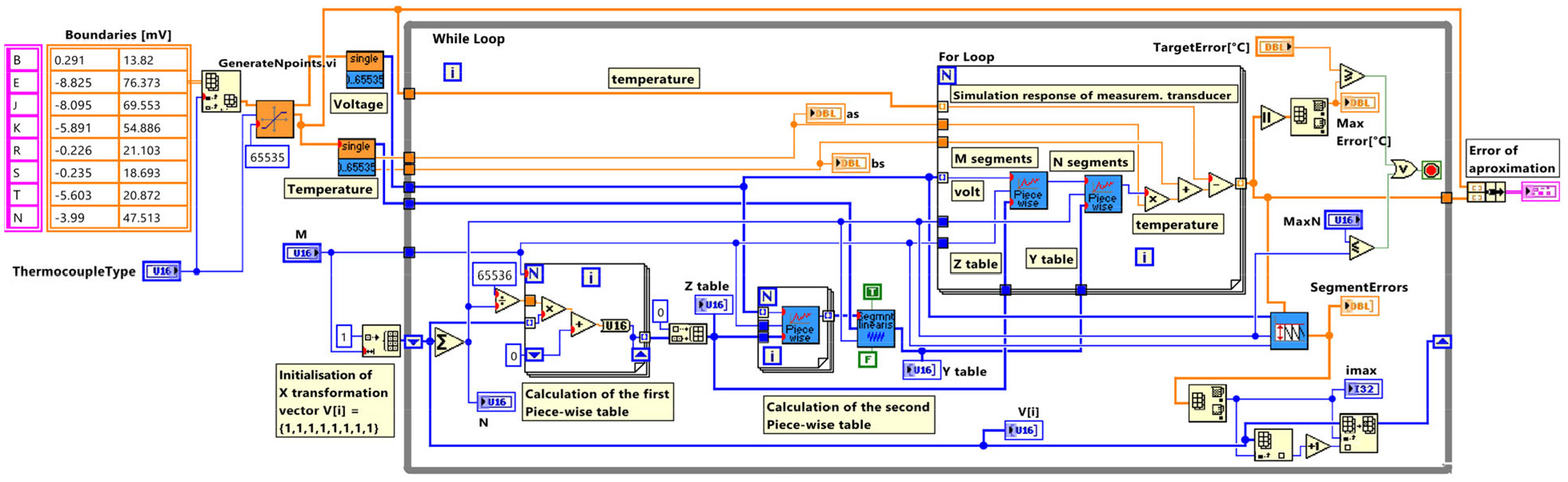
LabVIEW block diagram (software code) for iterative determination of the two-segment linearization tables, and calculation of the final approximation error.

On the left side of the block diagram, one can see the selection of a thermocouple type, which then selects corresponding endpoints of the input voltage measuring range. Based on the thermocouple selection, 65536 couples of points for voltage and temperature are generated in the defined voltage range, using thermocouple calculation functions, implemented in the LabVIEW software, according to NIST approximation polynomials. Then, these voltage and temperature values are normalized to the range from 0 to 65535.

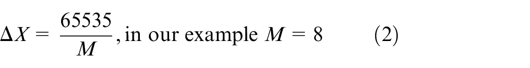
In the lower part of the block diagram, one can see the described procedure for obtaining the required Z and Y tables. Stretching the X-axis, that is, function Z_i = f₁(X_i) is based on the first piece-wise table, with the equal-sized X segments in the range from 0 to 65535. Each point on the X-axis is calculated as X_i = ΔX·i, for i = 0,…,M, where the value of segment ΔX can be calculated by the following equation:

Δ X = \frac{65535}{M}, in our example M = 8

(2)

Parameters of the new transformed function Z_i can be determined by the following calculations:

Z_{0} = 0, Z_{i} = Z_{i - 1} + V [i] Δ Z

(3)

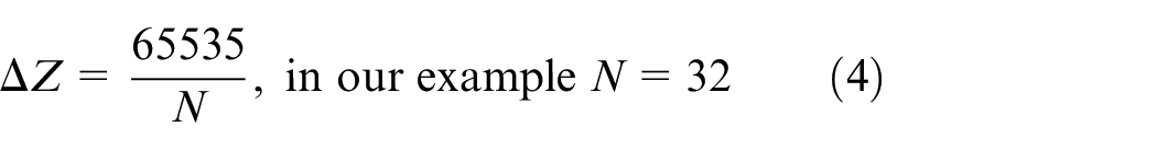
Segment ΔZ is calculated using the equation:

Δ Z = \frac{65535}{N}, in our example N = 32

(4)

The first linearization table is practically defined by the X transformation vector V[i], that is, array of coefficients in equation (3). For selected M = 8 segments of the first linearization table, initial value of this vector is V[i] = {1,1,1,1,1,1,1,1,1}. Such value of the vector means that the second linearization table has only one segment in each of the eight measurement voltage ranges. During the iteration process of the program, this vector is changed in a way that more nonlinear segments with bigger initial approximation errors increase V[i] numbers, which will be explained later.

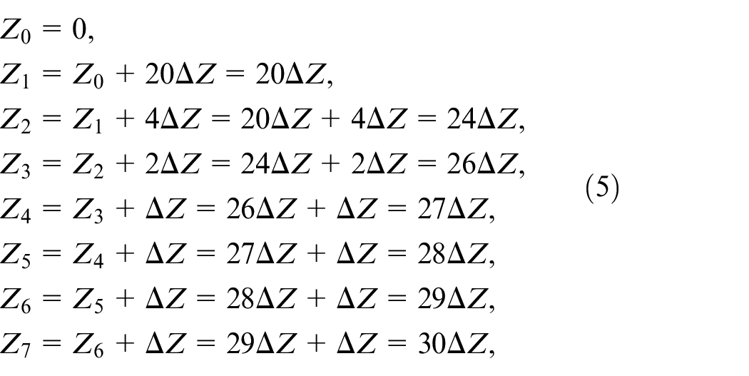
Transformation of the X-axis presented in Figure 3, for E type of a standard thermocouple is based on the final iteration result of the X transformation vector V[i] = {20, 4, 2, 1, 1, 1, 1, 2}, as presented at Figure 6 as the second row of the matrix, which contains finally reached coefficients for all types of thermocouples. The sum for all elements V[i] for each particular row is 32, based on the required number of the segments for the second piece-wise method. In this example, and by using V[i] according to relation (3), points of the Z table are calculated in the following manner:

\begin{matrix} Z_{0} = 0, \\ Z_{1} = Z_{0} + 20 Δ Z = 20 Δ Z, \\ Z_{2} = Z_{1} + 4 Δ Z = 20 Δ Z + 4 Δ Z = 24 Δ Z, \\ Z_{3} = Z_{2} + 2 Δ Z = 24 Δ Z + 2 Δ Z = 26 Δ Z, \\ Z_{4} = Z_{3} + Δ Z = 26 Δ Z + Δ Z = 27 Δ Z, \\ Z_{5} = Z_{4} + Δ Z = 27 Δ Z + Δ Z = 28 Δ Z, \\ Z_{6} = Z_{5} + Δ Z = 28 Δ Z + Δ Z = 29 Δ Z, \\ Z_{7} = Z_{6} + Δ Z = 29 Δ Z + Δ Z = 30 Δ Z, \end{matrix}

(5)

Figure 6.

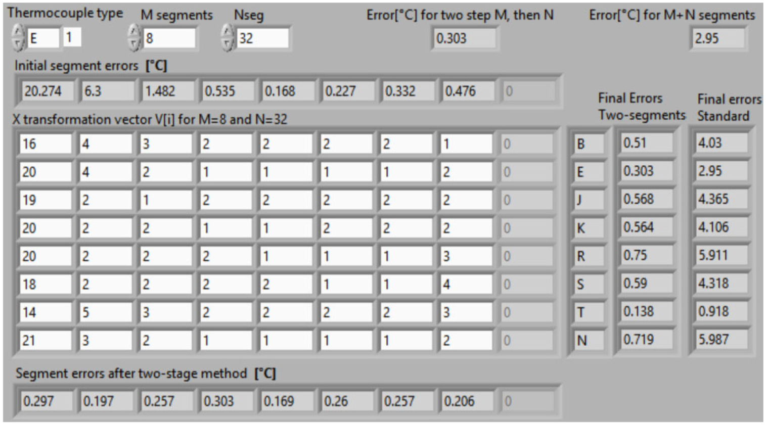
Front panel with coefficients for the first piece-wise table, and final errors comparison between two-stage 8 + 32 segments with standard 40 segments approximations, for eight standard types of thermocouples.

$Z_{8} = Z_{7} + 2 Δ Z = 30 Δ Z + 2 Δ Z = 32 Δ Z = 65536$ , used 65535 as a maximum – unsigned int16

Transformed X values, that is, Z = f₁(X), are calculated in the whole working range, based on the obtained Z table. The inverse transfer curve as a function of the transformed X-axis is then analyzed to determine the piece-wise approximation points for the 32 segments of the second stage linearization. This second piece-wise approximation, based on the least square deviation method is encapsulated inside a Sub VI block, same as the calculation of values based on the piece-wise table, named in the block diagram as “Segment Linearis” and “Piece_Wise.”

Based on the obtained Z and Y tables in the current iteration, a simulation of measurement transducer response in a “For Loop” is given at the right part of the block diagram. In those calculations, with a normalized input voltage as an input, in the range from 0 to 65535, a sub-VI performs the piece-wise calculation two times to approximate the inverse transfer characteristic. Finally, the obtained result is scaled back to the temperature value. In comparison to the temperatures obtained directly using the NIST polynomial, the approximation errors are calculated. Maximal errors of the approximation at each of eight segments form a vector named “SegmentErrors” in the block diagram. In the bottom of the block diagram, the LabVIEW functions whose job is to determine in which of the eight segments the error is the largest, are located. Once the segment with the biggest error, the segment “imax,” is determined, the iteration process increases the number of second linearization stage segments used on imax, V[imax]. The loop continues into the next iteration with a changed X transformation vector V[i], and in such way, that the total number of the segments N is increased by one.

In the example of E type of thermocouple, initial segment errors in degrees Celsius for each of the eight segments are 20.274, 6.3, 1.482, 0.535, 0.168, 0.227, 0.332, and 0.476, as can be seen in the top of Figure 6. It can be noticed that the maximal error of the piece-wise linear approximation is in the first segment, and it is 20.274°C. Thus, vector V[i] will be transformed from initial value to {2,1,1,1,1,1,1,1,1}, and so on, in iterative process up to previously mentioned final value of {20,4,2,1,1,1,1,1,2}. At this moment, the maximal error of approximation over the complete working range, 0.303°C will be achieved. This error can be seen in the fourth segment of the working range, Figure 6 bottom. Comparison of final approximation errors with a two-stage method using 8 + 32 segments, to one stage method with 40 segments for all eight standard types of thermocouples is given in Figure 6, right part of the front panel. The reduction of the errors is from 6 to 10 times. This final temperature approximation error obtained for the given example of E type of thermocouple, after completed two-stage linear approximation is significantly reduced from 2.95°C to 0.303°C, taking into account the same amount of the memory, that is, the total number of 40 segments.

The front panel with a graphical presentation of the obtained E-type thermocouple approximation errors for the two methods is given in Figure 7. The white colored curve shows the approximation error using the standard piece-wise method with 40 linearization segments. The diagram shown in red color presents the approximation error obtained after the complete procedure for two-stage linear segment approximation, where the first stage is based on eight segments, and the second on 32 segments. It can be seen that implementation of two-stage linear segment approximation enables a significant reduction of the thermocouple approximation error compared to the initial error value of the one-stage approximation, with the same number of table points used overall.

Figure 7.

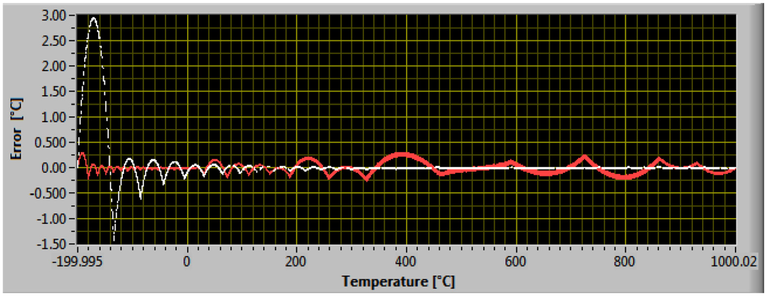
LabVIEW front panel with diagrams of obtained approximation errors after one-stage and two-stage linear segment approximation. White: one-stage, 8 + 32 = 40 segments; red: two-stage, eight, then 32 segments.

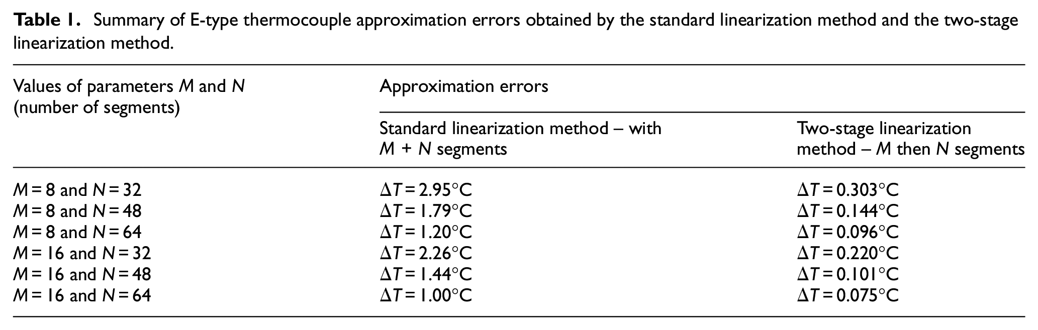
To make a more detailed comparison between the approximation errors using the standard piece-wise and the two-stage linearization method, additional calculations with various numbers of linearization segments (M and N) are performed for E-type thermocouple. The numbers of segments used in the comparison are: M = 8, M = 16, N = 32, N = 48, and N = 64. Obtained errors are presented in Table 1. It can be noticed that increasing the number of linearization segments slightly increases the advantage of the two-stage segment linearization method compared to the standard method with M + N segments. In the case of segment parameter values M = 8 and N = 32, the two-stage linearization method reduces approximation error 9.73 times, while for M = 16 and N = 64 this method reduces error 13.3 times.

Table 1.

Summary of E-type thermocouple approximation errors obtained by the standard linearization method and the two-stage linearization method.

Values of parameters M and N(number of segments)	Approximation errors
	Standard linearization method – withM + N segments	Two-stage linearization method –M then N segments
M = 8 and N = 32	ΔT = 2.95°C	ΔT = 0.303°C
M = 8 and N = 48	ΔT = 1.79°C	ΔT = 0.144°C
M = 8 and N = 64	ΔT = 1.20°C	ΔT = 0.096°C
M = 16 and N = 32	ΔT = 2.26°C	ΔT = 0.220°C
M = 16 and N = 48	ΔT = 1.44°C	ΔT = 0.101°C
M = 16 and N = 64	ΔT = 1.00°C	ΔT = 0.075°C

The comparison between the standard and the two-stage method is also given in graphical form at Figure 8, for thermocouple K in the whole working range from −200°C to 1372°C. Abscissa presents the overall number of segments used. As the number of used segments increases up to 8 + 86 segments, the two-stage method (red color) reaches an error up to 11 times smaller than the standard method, that is, an error of 0.1°C, compared to the error of the standard method, which is 1.14°C.

Figure 8.

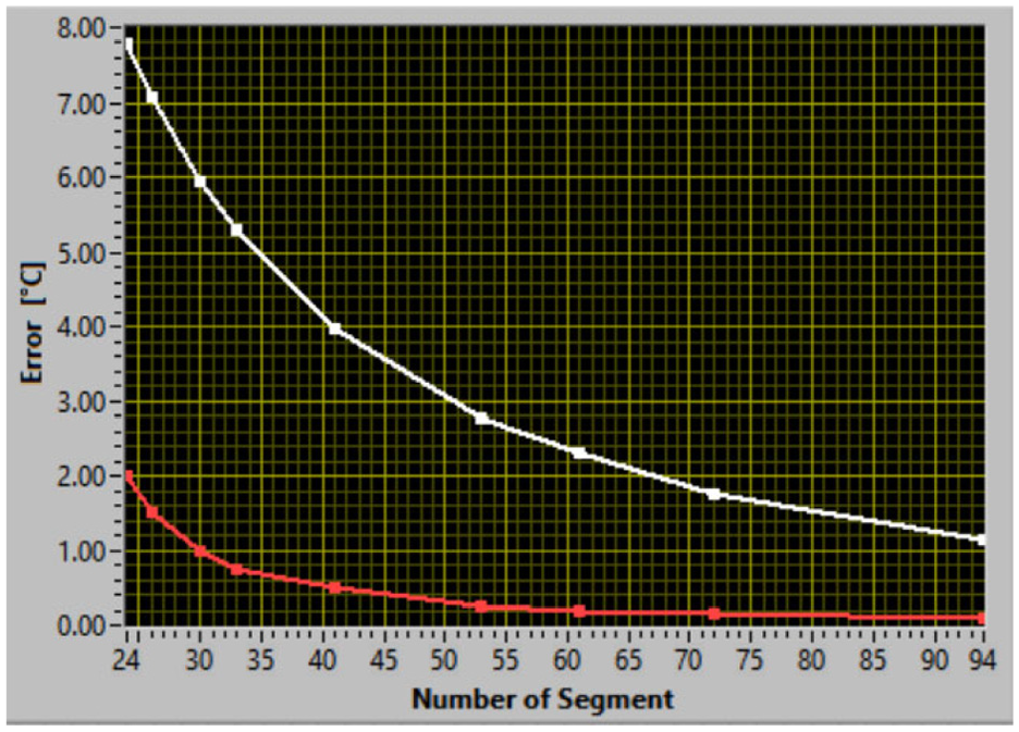
The approximation errors after one-stage (white) and two-stage (red) linear segment approximation for K type of thermocouple as a function of the overall number of segments.

The calculated linearization error for a different distribution of segments between M and N for thermocouple type S is given in Figure 9. There are 4 plots for different total number of segments (M + N) of 32 (white), 48 (red), 64 (blue), and 100 segments (green curve). On the abscissa is M, while the ordinate is the achieved approximation error. For a given total number of segments, M is in the range from 1 to (M+N)/2. For M = 1, when the whole input range is one segment, the error is the same as in the one-step method, while for the larger values of M, there are not enough segments left for the second linearization. It can be seen that in a wide range for the value of M between these two boundary cases, the error is weakly dependent on M, that is, for 100 segments it is almost the same from M = 8 to M = 41, for 64 segments the error is similar from M = 8 to M = 24. It is convenient to select M at the middle of this range of (N + M)/2 segments, that is, to select M = (N + M)/4, where the values for M is of the form 2^K (e.g. values 8 and 16) contribute to faster calculation. Anyway, this error is clearly smaller than for the one-step method error, as is shown in Figure 8.

Figure 9.

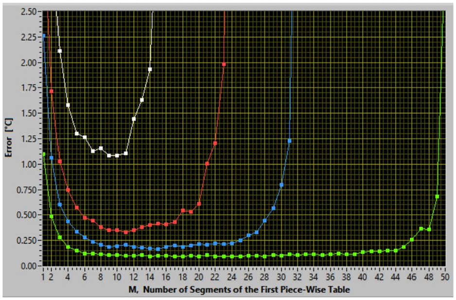
Approximation errors after two-stage method linear segment approximation as a function of the first piece-wise table size, for thermocouple type S. Four plots: M + N = 32 (white), 48 (red), 64 (blues), and 100 (green).

For a particular thermocouple, the whole temperature working range according to standard is considered, in the paper up to now. If a part of the operating range is required, the approach to linearization will be the same, the chosen range will always be stretched to the whole range of integer numbers that is, from 0 to 65535, and then the method will be implemented. However, a different error of approximation will be reached.

On the bar chart, Figure 10, the effect of reducing the operating range of type S thermocouple on the achieved error for standard linearization (number of segments 24, 32, and 48) and two-stage linearization with the corresponding number of segments of M = 8, and N = 16, 24, 40 is presented. The reduction of the range will relieve linearization, that is, decrease the number of segments to achieve the required error. With most thermocouples, not using part of the working range with negative temperatures, significantly reduces the error of the approximation, please see the third and fourth ranges in Figure 10.

Figure 10.

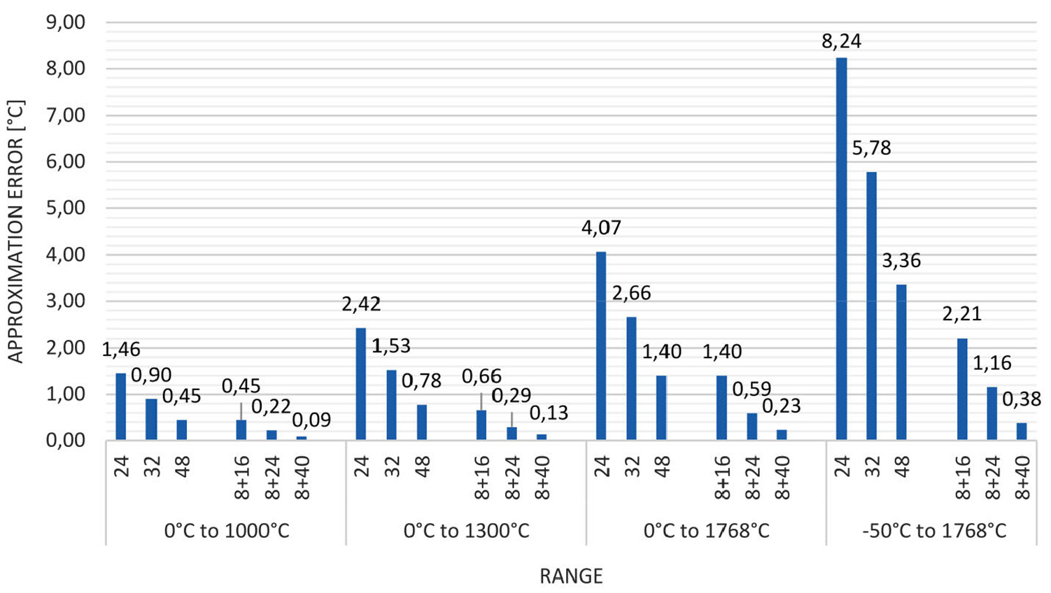
Approximation errors after one, and two-stage method linear segment approximation for different working ranges of thermocouple type S, and different number of segments.

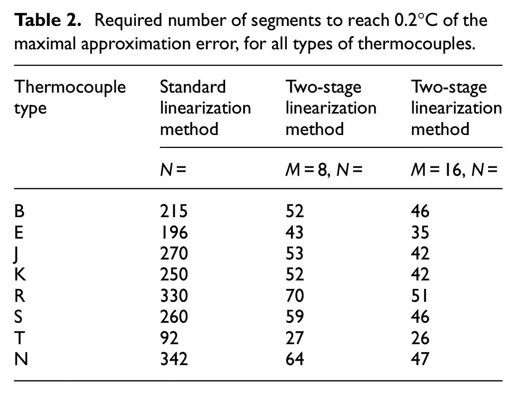
Taking into account other sources of errors in the thermocouple measurement chain, a goal error of 0.2°C can be a proper target value for the given iterative process of piece-wise tables calculation. In Table 2, the required number of segments for standard and two-steps piece-wise methods in order to reach this error is presented. The two-stage method is exposed by two columns in the table, with 8 and 16 segments in the first step.

Table 2.

Required number of segments to reach 0.2°C of the maximal approximation error, for all types of thermocouples.

Thermocoupletype	Standard linearization method	Two-stage linearization method	Two-stage linearization method
	N =	M = 8, N =	M = 16, N =
B	215	52	46
E	196	43	35
J	270	53	42
K	250	52	42
R	330	70	51
S	260	59	46
T	92	27	26
N	342	64	47

Conclusion

In the first part of the paper, the whole thermocouple measurement chain of a microprocessor transducer is presented and possible error is analysed in order to determine the required level of accuracy for the linearization of the transfer characteristics. The digital part of the measurement chain, that is, required calculations and data flow are pointed out. Inverse characteristic is used in the transducers, and analysed in the paper, as the goal is to calculate the temperature as function of the measured thermocouple voltage.

The linearization is implemented based on the two-stage piece-wise method proposed in Živanović et al.¹² The method is found appropriate for thermocouples, as the nonlinearity of the transfer characteristic is present in a different amount over the range of input values. LabVIEW software application for calculation of a linearization table coefficients and analysis of the obtained thermocouple approximation errors is explained in the paper. The basic principle of this two-stage linearization is to transform X-axis before final linearization in such a way that significantly nonlinear parts of the input range are expanded relative to the rest of the function.

In the calculations presented in the paper, the transformation of the X-axis is implemented based on an iterative process, where input is the final number of segments in the second piece-wise table, and linearization error is decreased by redistribution of the number of second stage segments which belong to particular segment used in the first transformation. The end of the iterative process can be also reached at the assigned maximal approximation error.

The proposed two-stage linearization method is compared to the standard piece-wise linearization method for the given examples of nonlinear transfer functions of standard thermocouples, with significantly better results. Using the two-stage approximation method for eight standard types of thermocouples: B, E, J, K, R, S, T, and N type, approximation errors are reduced from 6 to 13 times compared to the standard piece-wise method with similar execution time and equal memory consumption for storing the tables of linearization coefficients.

Presented linearization can be easily implemented by integer arithmetic, reducing the number of processor cycles required for calculations, and memory required for linearization tables and implementation of calculating procedures, in contrast to polynomial approximation, for example. The use of the two-step method is validated on the example of thermocouples. The presented iterative method can be used for two stage linearization of other sensor transfer characteristics.

Footnotes

Declaration of conflicting interests

The author(s) declared no potential conflicts of interest with respect to the research, authorship, and/or publication of this article.

Funding

The author(s) received no financial support for the research, authorship, and/or publication of this article.

ORCID iDs

Dragan Živanović

Milan Simić

References

Burns

Scroger

Strouse

, et al. NIST Monograph 175: Temperature-Electromotive Force Reference Functions and Tables for the Letter-Designated Thermocouple Types Based on the ITS-90, April 1993.

Bedford

Bonnier

Maas

Pavese

. Techniques for approximating the ITS-90, monograph BIPM, Bureau International des Poids et Mesures. Sèvres, France, 1990.

Measuresoft. DATASCAN 7000 distributed data acquisition system thermocouple accuracy, datascan.measuresoft.com/docs/TC.pdf (accessed November 2019).

Chen

Evaluation of piecewise polynomial equations for two types of thermocouples. Sensors 2013; 13(12): 17084–17097.

Wang

Wei

Sun

Free knot recursive B-spline for compensation of nonlinear smart sensors. Measurement 2011; 44(5): 888–894.

Nadi

Margo

Kouider

, et al. Embedded system design and implementation of standard auto-calibrated measurement chain. Int J Smart Sens Intell Syst 2008; 1(1): 21–33.

Danismana

Dalkirana

Celebib

FV.

Design of a high precision temperature measurement system based on artificial neural network for different thermocouple types. Measurement 2006; 39(8): 695–700.

Rivera

Carrillo

Chacón

, et al. Self-calibration and optimal response in intelligent sensors design based on artificial neural networks. Sensors 2007; 7(8): 1509–1529.

Dey

Munshi

A new intelligent scheme for simultaneous cold junction compensation and linearization of thermocouples. Leonardo Electron J Pract Technol 2011; 19: 13–28.

10.

Bengtsson

LE.

Lookup table optimization for sensor linearization in small embedded systems. J Sens Technol 2012; 2(4): 177–184.

11.

Erdem

Implementation of software-based sensor linearization algorithms on low-cost microcontrollers. ISA Trans 2010; 49(4): 552–558.

12.

Živanović

Arsić

Djordjević

Two-stage piece-wise linearization method. Int J Model Simul 2004; 24(2): 85–89.

13.

Grützmacher

Beichler

Hein

, et al. Time and memory efﬁcient online piecewise linear approximation of sensor signals. Sensors (Basel) 2018; 18(6): 1672.

14.

Sarma

Boruah

PK.

Design and development of a high precision thermocouple based smart industrial thermometer with on line linearisation and data logging feature. Measurement 2010; 43(10): 1589–1594.

15.

Islam

Mukhopadhyay

SC.

Linearization of the sensors characteristics: a review. Int J Smart Sens Intell Syst 2019; 12(1): 1–21.

16.

Živanović

Lukić

Denić

A novel linearization method of sin/cos sensor signals used for angular position determination. J Electr Eng Technol JEET 2014; 9(4): 1437–1445.

17.

Jovanović

Denić

A cost-effective method for resolution increase of the two-stage piecewise linear ADC used for sensor linearization. Meas Sci Rev 2016; 16(1): 28–34.

18.

JUMO GmbH & Co. KG. Data sheet 90.1000, Construction and application of thermocouples, www.jumo.net/attachments/JUMO/attachmentdownload?id=4121 (2009, accessed November 2019).

19.

Texas Instruments. TI designs, Optimized sensor linearization for thermocouple, www.ti.com/lit/ug/tidua11a/tidua11a.pdf (2015, accessed November 2019).

20.

Duff

Towey

Two ways to measure temperature using thermocouples feature simplicity, accuracy and flexibility. Analog Dialogue 2010; 44(10): 1–6.

21.

Živanović

Arsić

Djordjević

, et al. Two stages piece-wise linearization method for intelligent transducers. In: International scientific conference—ICEST 2003, Sofia, Bulgaria, December 2003, pp.383–386.

Two-stage segment linearization as part of the thermocouple measurement chain

Abstract

Keywords

Introduction

Thermocouple input stage

Introduction of the two-stage linear approximation method applied to standard thermocouples

Conclusion

Footnotes

Declaration of conflicting interests

Funding

ORCID iDs

References