
Abstract
In this paper, a short-term wind speed prediction model, called CEEMDAN-SE-Improved PIO-GRNN, is proposed to optimize the accuracy of the short-term wind speed forecast. This model is established on account of the optimized General Regression Neural Network (GRNN) method optimized by three algorithms, which are Complete Ensemble Empirical Mode Decomposition with Adaptive Noise (CEEMDAN), Sample Entropy (SE), and Pigeon Inspired Optimization (PIO), separately. Firstly, decomposing the original wind speed sequences into several subsequences with different complexity by CEEMDAN. Then, the complexity of each subsequence is judged by SE and the similar subsequences are combined into a new sequence to reduce the scale of calculation. Afterwards, the GRNN model optimized by improved PIO is used to predict each new sequence. Finally, the predicted results are superposed as the eventual predicted value. Implementing the prediction for the wind speed data of a wind field in north China within 30 days by applying the different prediction models, namely, GRNN, CEEMDAN-GRNN, Improved PIO-GRNN, and CEEMDAN-SE-Improved PIO-GRNN which are proposed in this paper. Comparing the prediction curves of different models with the fitting curve of the actual wind speed shows that the optimal fitting effect and minimum error value are included in CEEMDAN-SE-Improved PIO-GRNN model. Specifically, the values of mean squared error (MSE), mean absolute error (MAE) and weighted mean absolute percentage error (WMAPE) separately decrease by 0.6222, 0.3334, and 8.5766%, which compare with the single prediction model GRNN. Meanwhile, diebold-mariano (DM) test shows that the prediction ability of the two models is significantly different. The above statements indicate the proposed model does great advance in the precision of short-term wind speed prediction.
Keywords
Introduction
Time in recent decade, with the rapid deterioration of the global climate, the wind power, a kind of renewable clean energy, is gradually developed and utilized in many countries and cities because of its advantages of abundant reserves and wide distribution region.1,2 By the end of 2019, Europe’s cumulative installed capacity of wind power is 205 GW, accounting for 15% of Europe’s electricity demand. 3 China’s cumulative installed capacity is 210 GW, accounting for 32.3% of the total global installed capacity (650 GW). In the same year, the wind power generation of China also developed rapidly, with 26.2 GW of new installed capacity, accounting for 43.4% of the new global installed capacity (60.4 GW), ranking the first in the world.
Wind speed is one of the most important factors for wind power generation. Nevertheless, the fluctuation, stochasticity, and uncontrollability of wind speed result in the instability for wind power, the difficulties in grid connection and wind turbines control problems, which all will pose huge difficulty to the stable and safe operation for the power system. The precise short-term wind speed prediction can not only decrease some operation cost for the power network, but also is beneficial for power system departments to conduct power dispatch. 4
In recent decades, physical methods 5 and statistical methods 6 are mainly used to optimize the precision of wind speed prediction. The physical method mainly uses the numerical weather forecast data, establishes the expression through the relation of wind speed and air pressure, air density, air humidity, and so on. Finally, the wind speed forecast is realized. However, due to the high complexity of wind speed and regional differences in wind location, it is difficult to establish high-precision short-term prediction for different regions. Comparatively, the mathematical model of the statistical method involves time series analysis, which is more accurate than the physical method to realize the short-term wind speed forecast. Time series prediction method, based on the time series of historical statistical data, predicts, and analyzes the future trend of change. This method uses the historical data of wind speed to establish the mapping relationship between the input and output of the system, and predicts the future wind speed. This modeling process is simple and feasible with low cost. 7
Literature 8 applied WD (Wavelet Decomposition) and AdaBoost neural network to implement wind speed short-term prediction. However, the effect of WD is influenced by the selection of wavelet base and decomposition scale. Once determined, the result obtained by decomposition is fixed frequency band, 9 and the range of this frequency band is only related to the sampling period. Hence, it does not have self-adaptability. Compared with this defect, literature 10 used EMD and CNNSVM (Convolutional Support Vector Machine) to conduct wind speed short-term prediction. Specially, EMD was used to extract the fluctuation characteristics of wind speed data and decompose the time series of wind speed into several sub- sequences. Although EMD has strong self-adaptability, there are phenomena of modal aliasing, over-envelope and under envelope. In order to suppress these, the hybrid model including data processing, data clustering and data prediction in literature 11 was proposed to predict future wind speed data. Among them, Kerny-based Fuzzy C-means Clustering was applied in data clustering, data prediction is applied in Wavelet Neural Networks, and data processing is applied in EEMD. However, the amplitude selection of this noise is very important. If it is too low, modal aliasing cannot be suppressed; On the contrary, calculation amount will be increased and more pseudo-components will appear. In normal, the amplitude is selected according to human experience, which leads to certain errors in decomposition.
Compared with EEMD, the adaptive gaussian white noise is appended in each stage through the CEEMDAN.12–14 Each modal component is obtained through operating the unique residual signal, which effectively figures out the problem of low decomposition efficiency for EEMD and the difficulty of completely eliminating the noise.
The following contents are the contributions of this paper:
In view of strong instability and volatility for the original wind speed sequence, CEEMDAN is employed to decompose it into a sequence of IMF components with different complexity. However, there are many similar complexity IMF components. If a prediction model is established for each IMF, it will not only increase the amount of modeling and the time of prediction, but also accumulate errors in the final superposition process and reduce the accuracy of prediction. Therefore, SE is used to quantify the degree of irregularity of each IMF component, and sequences with similar SE values are combined to enhance the speed and precision for forecast.
GRNN model is used to predict the new combined sequence, but traditional GRNN needed to be tested and compared again and again to determine the size of the smooth factor in the kernel function of hidden regression unit. In this paper, the PIO algorithm is introduced to automatically optimize the smooth factor of GRNN.
The original PIO is prone to trap its result in a local optimum, which is essential to be optimized. A dynamic adaptive geomagnetic operator based on an objective function is proposed to replace the method of setting a fixed value of R for a geomagnetic operator in the original method. The performances of improved PIO, standard PIO and standard PSO are respectively tested by four kinds of nonlinear multi-peak function. By comparing the algorithm optimization performance diagram, optimal solutions, the worst values, the mean values, and the variance values, it shows that the improvements of PIO algorithm can effectively alleviate the issue which the algorithm is prone to trap its result in a local optimum, and is able to strengthen the optimization speed and accuracy for the algorithm.
The prediction model is established based on CEEMDAN-SE-Improved PIO-GRNN. The wind speed data which derived from a power plant in north China within 30 days is employed to implement the simulation experiment by the different models, namely, GRNN, Improved PIO-GRNN, CEEMDAN-GRNN, CEEMDAN-SE-GRNN, and CEEMDAN-SE-Improved PIO-GRNN. The comparison of the prediction curves, and following error evaluation criteria, which is MSE, MAE and WMAPE, certificates the proposed model possesses the superior prediction effect.
The following is the organization for the remaining paper. The section 2 presents the wind speed data’s source and the pretreatment and complexity analysis method. The section 3 introduces the establishment of the prediction model, including model establishment, model parameter optimization method and improvement of the optimization method. The simulation analysis is implemented in the section 4. The section 5 summarizes the full text.
Preprocessing and complexity analysis of wind speed data
The data sources
For wind speed prediction, total 2880 sets of wind speed data, which were collected at 15-min sampling intervals in January from a wind field of Zhangjiakou city located between north China plain and inner Mongolia plateau, were selected. Figure 1 shows the sequence for the wind speed data.
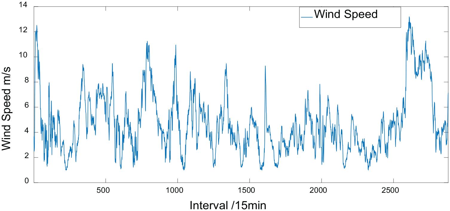
Wind speed data sequence diagram.
It could be discovered in Figure 1 that the wind speed sequence involves the feature of strongly instable and fluctuant, which is the reason why it is difficult to capture its characteristics with a single prediction model, thereby affecting the prediction accuracy.
Complete ensemble empirical mode decomposition with adaptive noise
Aiming at the problem of strong fluctuation of wind speed data in north China wind field, Complete Empirical Mode Decomposition with Adaptive Noise (CEEMDAN) algorithm 15 was adopted to decompose the wind speed sequence with strong instability into a series of eigenmode functions to reduce its fluctuation. It is widely used in processing nonlinear and nonstationary signals because it synchronously overcomes the problem of EMD mode aliasing and the difficulty of determining the amplitude of Gaussian white noise in EEMD decomposition. Specially, it has a better effect in the decomposition of wind speed sequence, so it has a greater advantage. The principle of this algorithm is as follows:
The white noise sequence
1) Add white noise
At this point, the residual signal
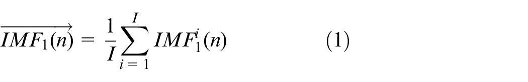
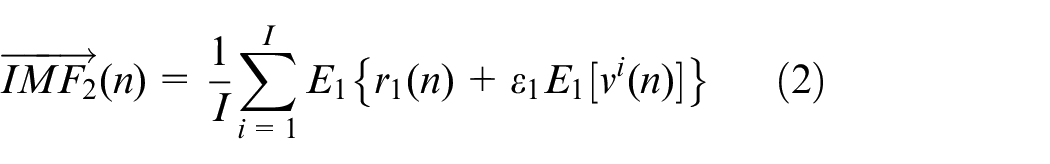
2) Add the IMF component
3) The k-th residual signal
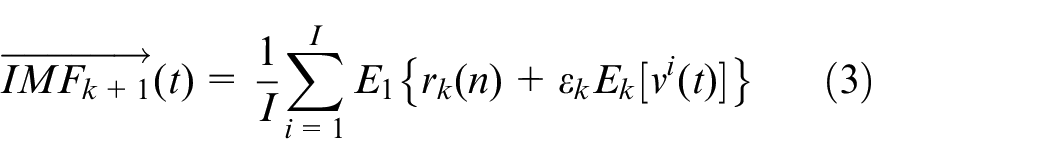
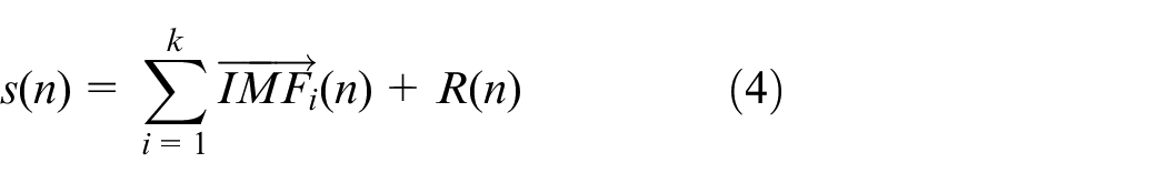
4) Repeat step 3 until the remaining components fail to meet the decomposition conditions of EMD. Eventually, the original signal is decomposed as follows:
Sample entropy calculation for each IMF component
To resolve the issue that many sequences with similar complexity are produced after CEEMDAN decomposition, the Sample Entropy is applied to quantify the complexity of each IMF component.
Sequences with similar SE values also include similar complexity and wind speed characteristics. Hence, SE values can be selected as indicators to classify IMF components, and combine the sequences with similar SE values. Consequently, it can avoid redundancy, reduce error accumulation, and improve the prediction speed and accuracy.
Sample Entropy (SE)16–18 is an improved method for measuring the complexity of time series based on Approximate Entropy (ApEn) proposed by Richman et al. It is easy to calculate and extremely fast, which has an excellent effect on the calculation of long data series.
Set a time series consisted of N points, which can be defined as
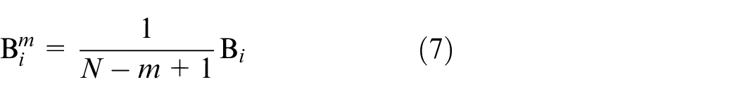
1) (N-m+1) m-dimensional vector

where
2)

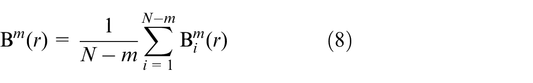
3) Given a threshold
4) Take the mean value for all
5) Increase the dimension by 1. That is, when dimension is
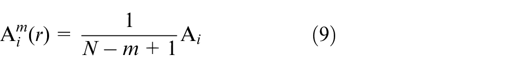
where
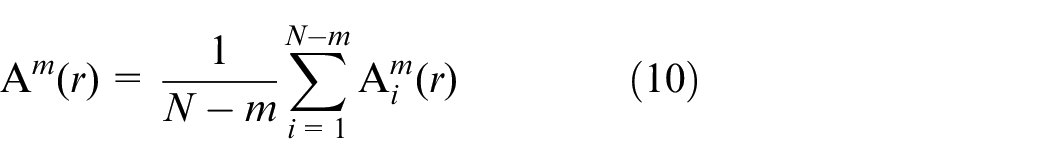
6) Therefore, when the threshold

When N is set as a finite value, the estimated value of SE is as equation (12):

For each IMF component, SE is used to quantify the clutter degree to provide theoretical basis for the combination of IMF components and simplification of model in subsequent steps. Specifically, the larger the SE values, the stronger the randomness of the sequences, and vice versa. 19
Establishment of PIO-GRNN prediction model
General regression neural network
In this paper, General Regression Neural Network (GRNN) is used to predict the above combined IMF sequences. GRNN20,21 is an improved radial basis neural network. Compared with other traditional neural networks, GRNN is more suitable for predicting nonlinear and nonstationary sequences with the advantages of faster computation speed, greater fault tolerance and better robustness.
In Figure 2, it could found that the GRNN is simply consisted of four layers, namely, the input layer, the pattern layer, the summation layer, and the output layer
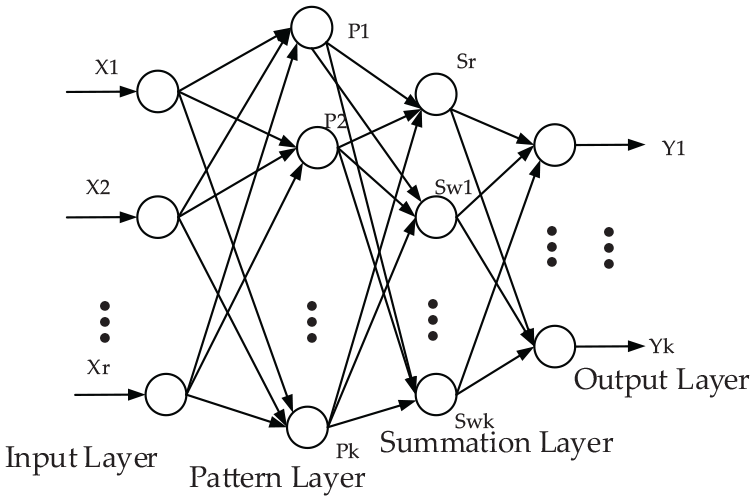
The structure of GRNN.
Input layer
In the learning sample, the counts of the input layer’s neurons are equivalent to the input vector’s dimension. For each neuron, the input variable is directly passed to the pattern layer as a simple distribution unit.22,23
Pattern layer
The counts of pattern layer’s neurons are equivalent to the counts of learning samples n. Specifically, each neuron corresponds to diverse samples. The transfer function for i-th pattern layer’s neuron is as follows 24 :
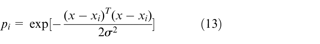
where
Summation layer
In the summation layer, two kinds of neurons are involved. For one kind of neuron, the transfer function can be shown as follows:
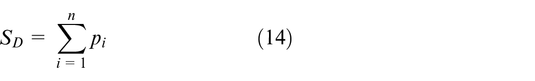
For output of each neuron in the pattern layer, conducting the arithmetic sum. For another kind of neuron, the transfer function is shown as follows:
where
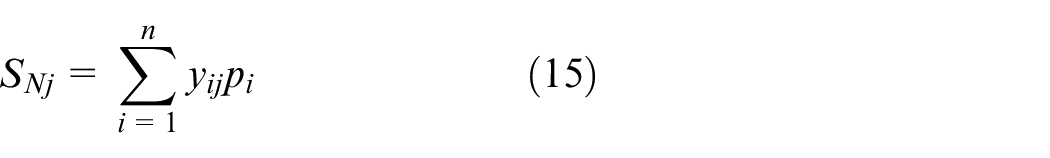
For the outputs of pattern layer’s each neuron, they are weighted and summed by using the equation (15), where
Output layer
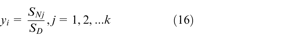
The counts of output layer’s neurons are equivalent to the output vector’s dimension in the learning sample. The output result is the quotient of the results obtained by the two kinds of summation methods in the summation layer, namely:
Parameters optimization for GRNN based on pigeon inspired optimization
Standard pigeon inspired optimization
By studying the model of GRNN can be found that there are relatively few factors that need manual adjustment. However, the value of the smoothing factor
Pigeon Inspired Optimization (PIO)25,26 was proposed by professor Duane Haibin in 2014. This algorithm derives from simulating the homing behavior of pigeons. The pigeons determine the general direction through the geomagnetic field in priority. Then the actual direction is corrected according to the practical geomorphic landscape. Eventually, they can accurately locate the nest location. The specific steps are as follows:
1) Initialize spatial dimension D, population scale
2) Set the random speed and route for each pigeon. Then implement the operation of the fitness value for each pigeon to find the best route.
3) Determine the approximate flight direction according to the geomagnetic field. Update the speed and route of each pigeon based on the following formulas. After calculating the updated pigeon’s fitness value, the best novel route can be searched.
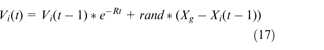

where t is the counts of current iteration, R is geomagnetic operator,
4) If
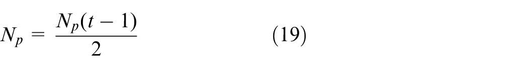
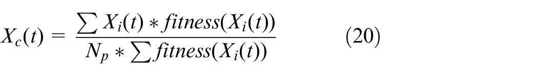
5) Firstly, sorting the fitness values of the pigeons by descending order. Then, halving the pigeons with low fitness according to equation (19). Moreover, finding the center of the remaining pigeons, namely, the ideal destination, according to the equation (20). Eventually, adjusting the specific flight direction according to the equation (21) when all pigeons arrive at the destination.

6) If
Improved pigeon inspired optimization
Compared with other swarm intelligence optimization algorithms, the PIO includes the advantages of concise principle, strong robustness, fewer parameters to tune, easily implementing and rapid convergence speed. However, there may be still some problems with this algorithm, such as, low convergence accuracy, easily falling into local optimum, 27 and relatively poor stability. Therefore, the adaptive geomagnetic operator is proposed for optimizing PIO.
The standard PIO possesses the advantages of less arguments and easily implementing. Meanwhile, the algorithm still contains the disadvantages of poor convergence precision and easily trapping in the local optimum. To get rid of the local optimum, it is vital to select the geomagnetic operator R. The value of
In this paper, the method of setting fixed value for the geomagnetic operator R in the original method is abandoned. Instead, a dynamic adaptive geomagnetic operator based on objective function is proposed. In priority,
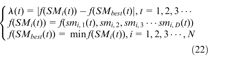
where the iterations times of the pigeons is expressed as t.
What’s more, the geomagnetic operator R can be calculated by the equation (23).
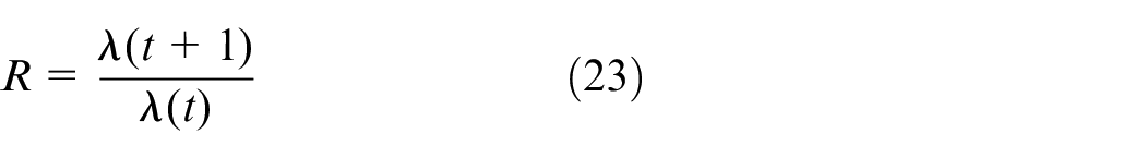
where
Equation (23) is used to calculate the geomagnetic operator, which results in the change of geomagnetic operator is relatively smooth and varies within the range of [0,1]. As the value of
Forecasting process
To validate the availability of the model, a wind speed prediction model based on CEEMDAN-SE-Improved PIO-GRNN is established. Under situation
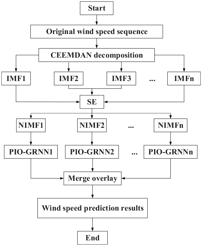
Wind speed prediction flow chart based on CEEMDAN-SE-Improved PIO-GRNN.
The specific implementation steps are as follows:
To carry out the stabilization of the wind speed sequence, the original wind speed sequence is decomposed by CEEMDAN technology to generate a series of IMF components with disparate characteristic scales.
Furthermore, calculating the SE of each IMF component. Then, the IMF components with similar entropy are combined to form a new component, which reduces the calculation scale of the prediction model and the error accumulation.
In addition, the smoothing factor of GRNN is optimized with improved PIO algorithm. Assuming that the summation of output error’s absolute value from GRNN model’s training data is set as fitness function. Next, operating the Improved PIO-GRNN prediction for each new component.
Each new component’s predicted values are weighted and combined to achieve the result of the original wind speed prediction.
Simulation analysis
To validate the rationality for the proposed model, the actual measured historical data mentioned in section I are applied for simulation experiment. Total 2880 sets of windspeed data collected at 15-min sampling intervals are selected to establish the prediction model. Data from days 1 to 29, namely, 2784 sets of data, are applied to train models, and the remaining 96 sets of data are utilized to forecast the wind speed in coming day. Specially, the simulation is carried out on MATLAB 2016a platform.
The actually measured wind speed data shown in Figure 1 are highly nonlinear and volatile. For the purpose of fully grasping the variation characteristics of the original wind speed sequences, the wind speed sequences are decomposed by CEEMDAN. The added white noise can be set as follows: the noise amplitude is 0.2 times of the standard deviation for the sequences which waiting to be decomposed, the number of white noise additions is 100, and the number of iterations is 1000. The white noise added in the second and third decomposition is shown in Figures 4 and 5, and the residual generated by each decomposition is shown in Figure 6.
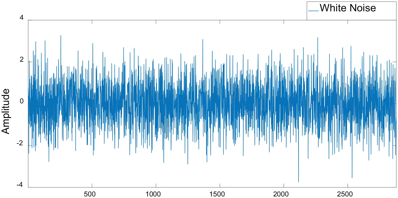
The white noise added during the second decomposition.
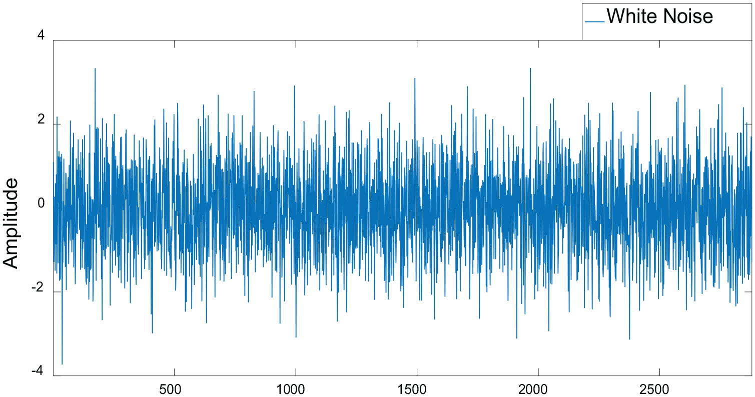
The white noise added during the third decomposition.
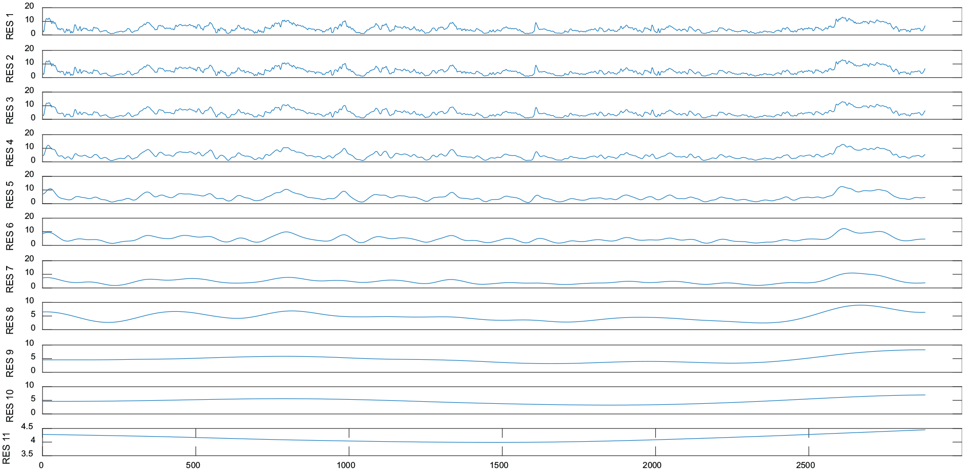
The residual diagram of each order decomposition.
The original wind speed sequence is decomposed by CEEMDAN to generate a series of IMF components with different complexity, which are displayed in the Figure 7.
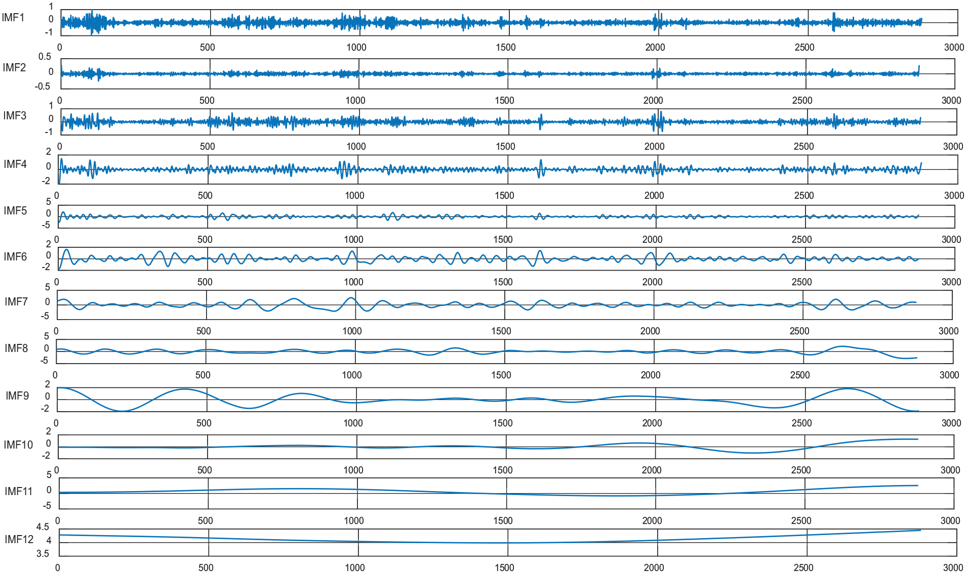
CEEMDAN decomposition diagram.
Nevertheless, it could be discovered from Figure 7 that the wind speed sequence obviously retains non-stationary, including many IMF components, among which IMF1 can be characterized by the highest frequency, the strongest randomness of the sequences and the maximum complexity; Relatively, IMF12 can be characterized by the lowest frequency, the strongest regularity of the sequences, and the minimum complexity. It would increase the superposition of errors if each component is predicted directly and the predicted results are superposed. To reduce the scale of modeling and the accumulation of errors, SE is introduced. After decomposing each modal component by CEEMDAN, each decomposed component is calculated to obtain the SE values and analyzed the complexity. Then, the sequences with similar SE values are merged into new sequences. Eventually, implementing the wind speed prediction by the proposed model.
It can be seen from the flow of SE algorithm that two important parameters directly affect the calculation results, namely, similar tolerance
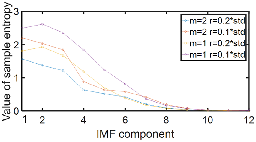
The SE of the IMF.
As is revealed in the Figure 8, when
Under the situation
The SE values of 12 modal components.
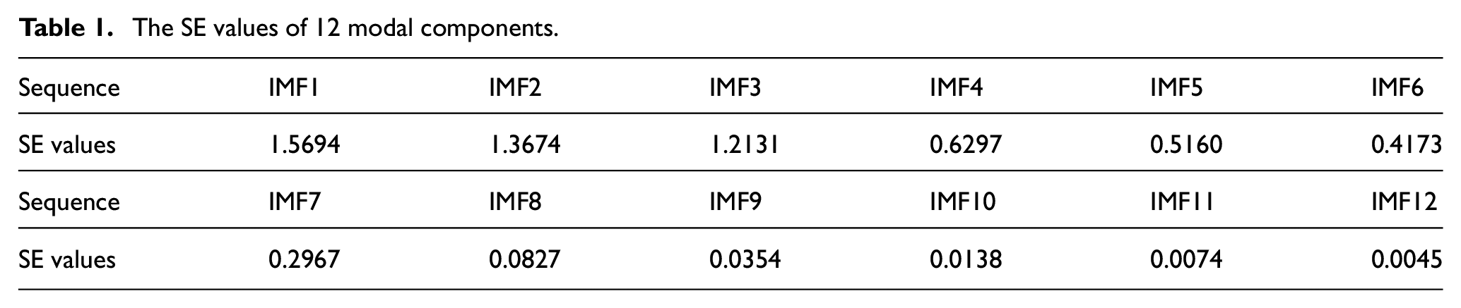
The larger the SE value, the greater the complexity of the corresponding sequence. The closer the SE values are, the closer the corresponding subsequences’ complexities are. As is shown in the Table 1, IMF1 possesses the maximum SE value, and IMF12 possesses the minimum one. This is consistent with the result obtained by observing the complexity of the modal components in Figure 4.
IMF1, IMF2, and IMF3 are characterized by high complexity, strong randomness for sequences, and significantly higher entropy values than other components. Therefore, they can be restructured as component NIMF1. The waveforms of IMF4, IMF5, IMF6, and IMF7 reveal the certain randomness, and their entropy values are similar, which can be merged into component NIMF2. The waveforms of IMF8 and IMF9 show the regularity, and their entropy values are relatively similar with each other. Therefore, they are restructured as component NIMF3. The waveforms of IMF10, IMF11, and IMF12 tend to be gentle, and the entropy value approaches 0, so they can be reconstituted into component NIMF4.
After the decomposition by CEEMDAN, modal components are recombined with better stability and smoothness. And it is also more convenient to extract the variation rules of the wind speed sequences.
Improved PIO algorithm
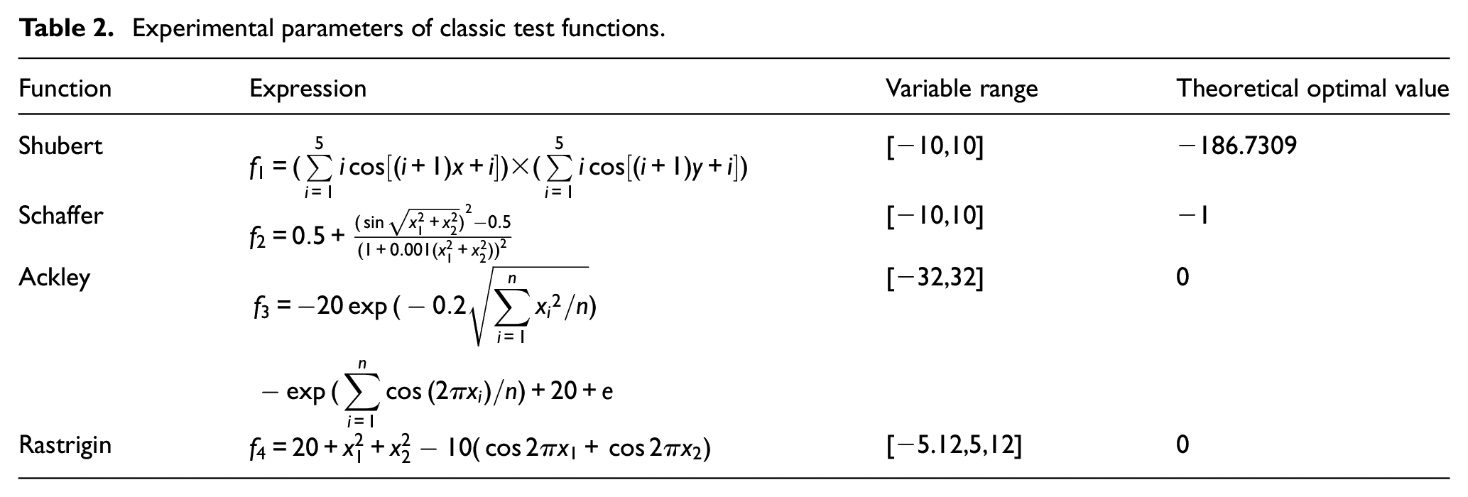
In this paper, the smoothing factor of GRNN is enhanced by the improved PIO. For the sake of verifying the advantages of improved PIO algorithm, four diverse classical test functions are selected to be simulated and tested by improved PIO, standard PIO, and standard PSO, separately. 50 times independent experiments should be operated for each algorithm. The four kinds of test functions totally are complicated nonlinear multi-peak functions, which are equipped with a mass of multiple local optimal solutions, and the capability of effectively checking global search for the algorithm and getting rid of the local optimal.
The expressions, range of variables, and ideal optimal values are shown in the Table 2.
Experimental parameters of classic test functions.
The four test functions will be separately operated 50 times independent experiments. In each independent experiment, the population number is 20 and cycle times are 200. Then, the optimal population solutions are achieved and shown in Figure 9, in which the x-axis presents the experiments’ counts, and the y-axis denotes the optimal solution. It is prone to obtain that the optimum curve of improved PIO closely approaches to the optimal solution. In detail, the minimum number of results trapped in the local optimum occurs in the improved PIO, which indicating that the improved PIO algorithm is easier to avoid the local optimum.
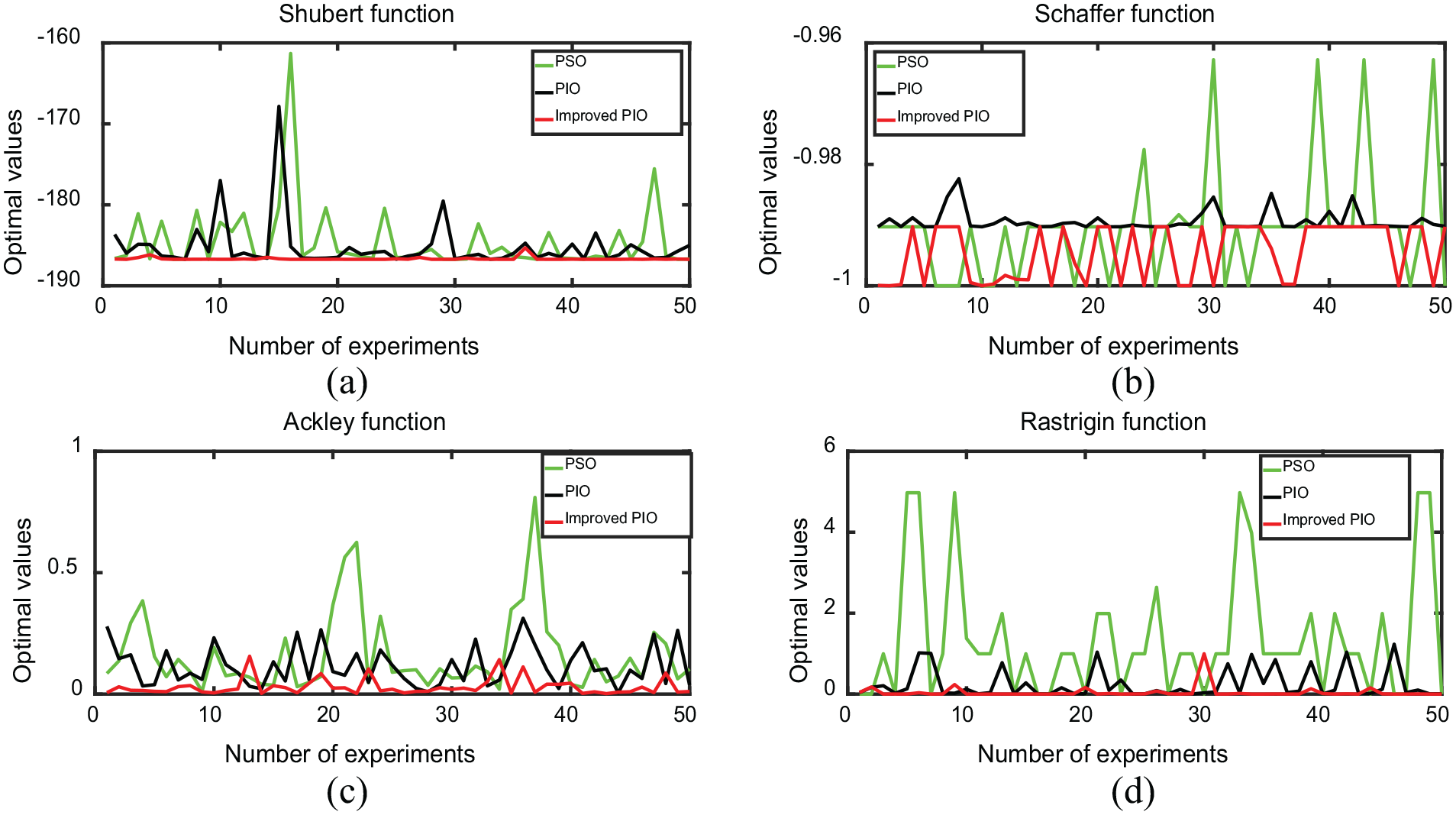
The comparison diagram of three algorithms optimization: (a) convergence curve of Shubert function, (b) convergence curve of Schaffer function, (c) convergence curve of Ackley function, and (d) convergence curve of Rastrigin function.
To further evaluate the performance of the improved PIO, each test function is independently operated for 50 times to obtain the optimum solution, the worst solution, mean value, and the variance from the optimized results. The algorithm performances for PSO, PIO, and improved PIO are compared and displayed in Table 3, where the optimum results of each function are highlighted in bold.
The comparison of three algorithms.
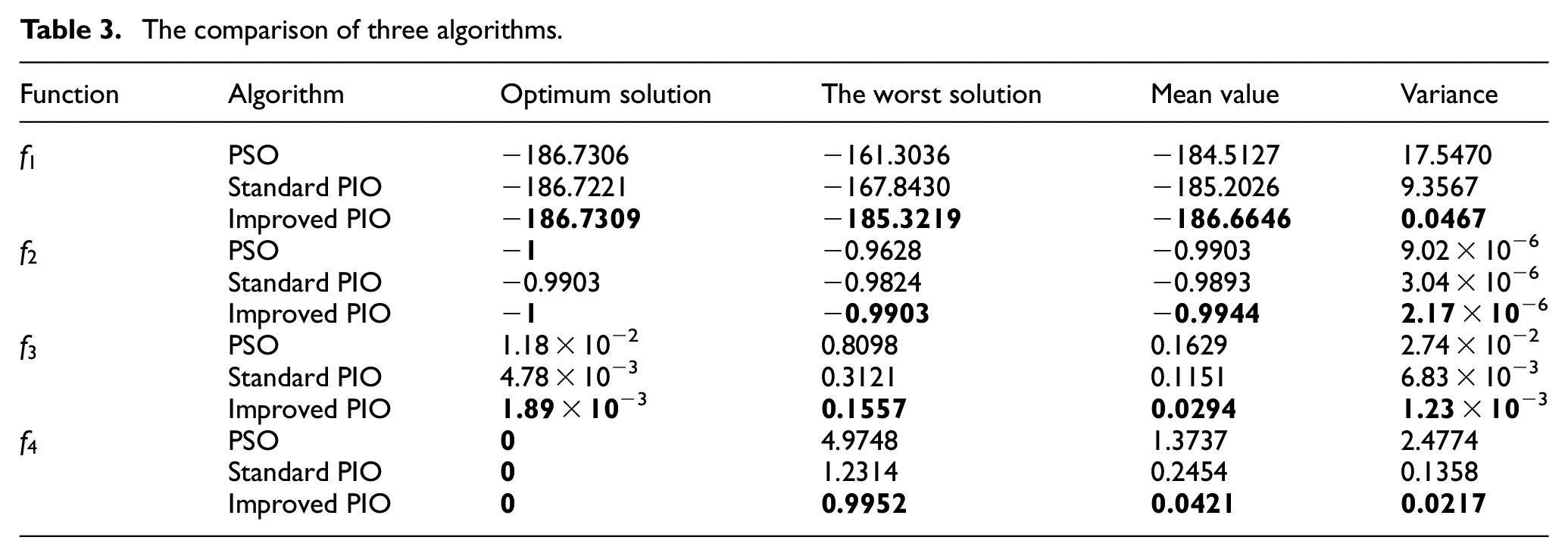
With regard to the four multimodal functions
According to the above diagrams, it can be learned that the optimization accuracy and stability of the PIO can be enhanced through improved PIO algorithm, and prevent the algorithm from being trapped in the local optimum. In sum, the improved PIO algorithm is effective and applicable for the complex function optimization problem.
The wind speed prediction based on CEEMDAN-Se-improved-PIO-GRNN
The Improved PIO-GRNN models are established for four new modal components to implement the forecasting. After the prediction, the each NIMF component’s results are superimposed and merged to achieve the final prediction results, which are displayed in Figure 10(a–d). Obviously, the overall fitting degree of NIMF1 is not satisfied because of the largest prediction error among all modal components. Relatively, the result of NIMF2 has been improved to a certain extent. However, there are still some problems happened to the positions of wave crest, wave trough, and the transition. The overall prediction result of NIMF3 is better than NIMF1 and NIMF2. However, a slight deviation happened in the prediction of wind speed in the last hour. By overall comparison, the fitting effect of NIMF4 is the best one with rare deviation from the actual wind speed.
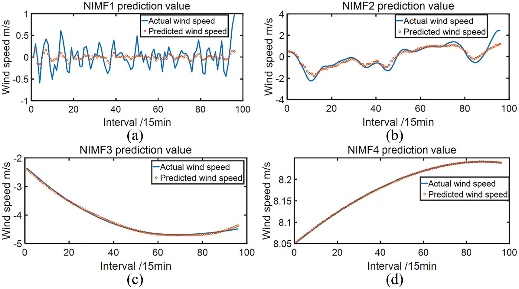
The prediction results for four new sequences: (a) prediction result of NIMF1, (b) prediction result of NIMF2, (c) prediction result of NIMF3, and (d) prediction result of NIMF4.
By superimposing the above prediction results, the final prediction results can be obtained, which are displayed in CEEMDAN-SE-Improved PIO-GRNN curve of Figure 12.
For verifying the superiority of the proposed model, five diverse models are separately established to operate the prediction for the 30-days data derived from a wind farm in north China. The models are GRNN, CEEMDAN-GRNN, CEEMDAN-SE-GRNN, Improved PIO-GRNN, and CEEMDAN- SE-Improved PIO-GRNN, respectively. For the sake of more intuitionistic comparison, the fitting degree of the predicted value and the actual value for each model are displayed in Figures 11 and 12.
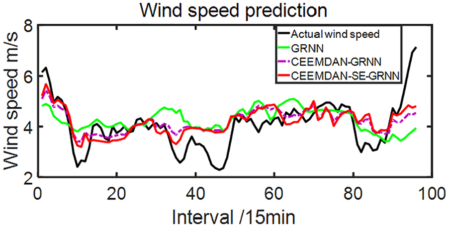
Prediction results diagram.
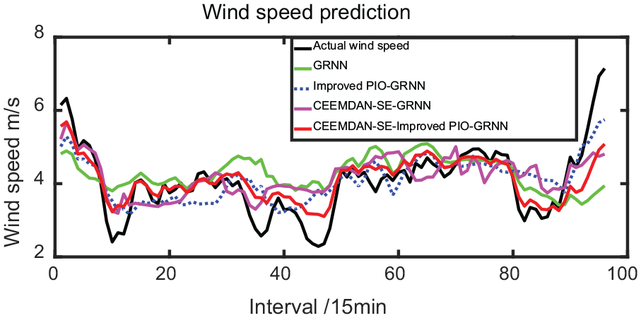
Prediction results diagram.
As can be seen from Figure 11, the fitting effect of CEEMDAN-GRNN prediction curve is better than the one of GRNN, and the fitting degree of CEEMDAN-SE-GRNN model is close to that of CEEMDAN-GRNN model. It can be seen from Figure 12 that Improved PIO-GRNN model has better prediction effect than GRNN. The CEEMDAN- SE-Improved PIO-GRNN has the best prediction curve fitting effect, and can be well predicted at both peak and trough.
If solely depending on the fitting degree of wind speed curve, it will be difficult to know by which method the best prediction effect can be obtained. Hence, it is necessary to judge the merits and demerits for each method according to several error evaluation criteria. Mean squared error (MSE), 31 mean absolute error (MAE) 32 and weighted mean absolute percentage error (WMAPE) 33 are three different indicators, which can be applied to estimate the prediction outcomes. The tinier the values of the three indicators are, the more precise the prediction accuracy of the model will be. The following expressions are the three error indicators.
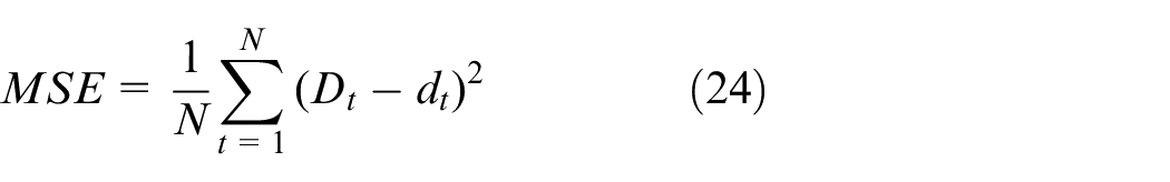
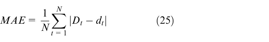
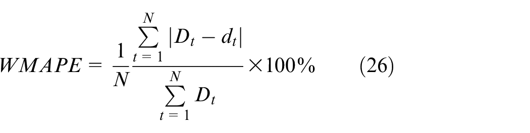
where
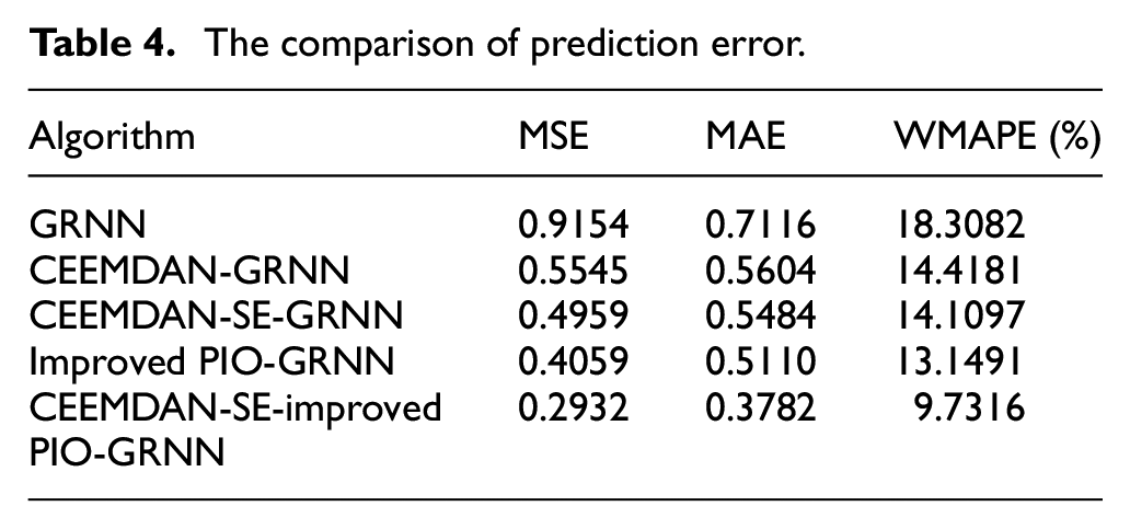
It can be seen from Table 4 that MSE, MAE and WMAPE have consistent evaluation on the predictive ability of the five prediction models. The descending order of predictive power is as follows: CEEMDAN-SE-Improved PIO-GRNN > Improved PIO-GRNN > CEEMDAN-SE-GRNN > CEEMDAN-GRNN > GRNN.
The comparison of prediction error.
The larger the value of the commonly used prediction evaluation indicator, the easier it is to see the difference in the predictive power of each model. However, what extent can be decided to judge it needs to be verified by DM test. To avoid the length of paper too long, specific theory will not be elaborated in detail in this paper. Please refer to the literature.34–36 By means of DM test, quantitative test can be carried out, so that it is easier to see the difference of prediction ability for each model. Only when the numerical difference of the above indicators for the models is significantly greater than 0, the predictive ability of one certain model is sufficient to be considered superior to other models.
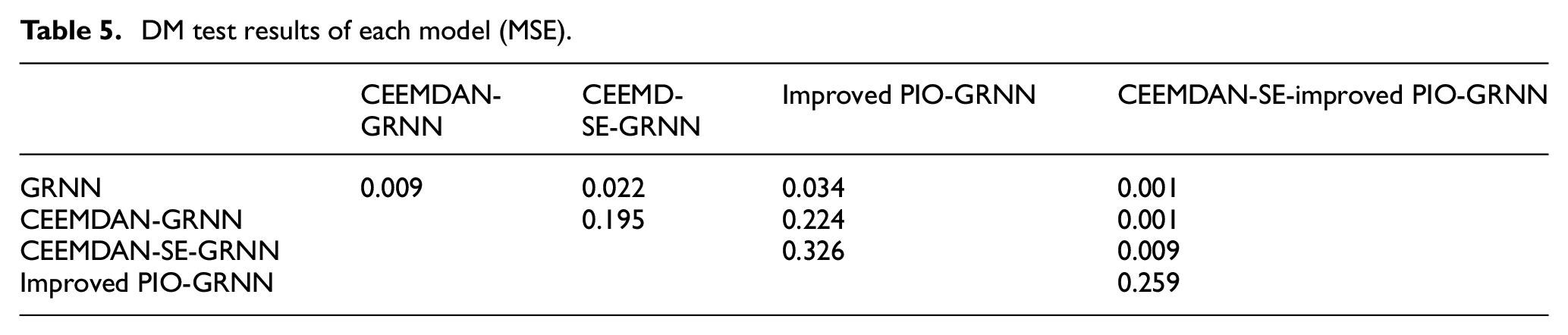
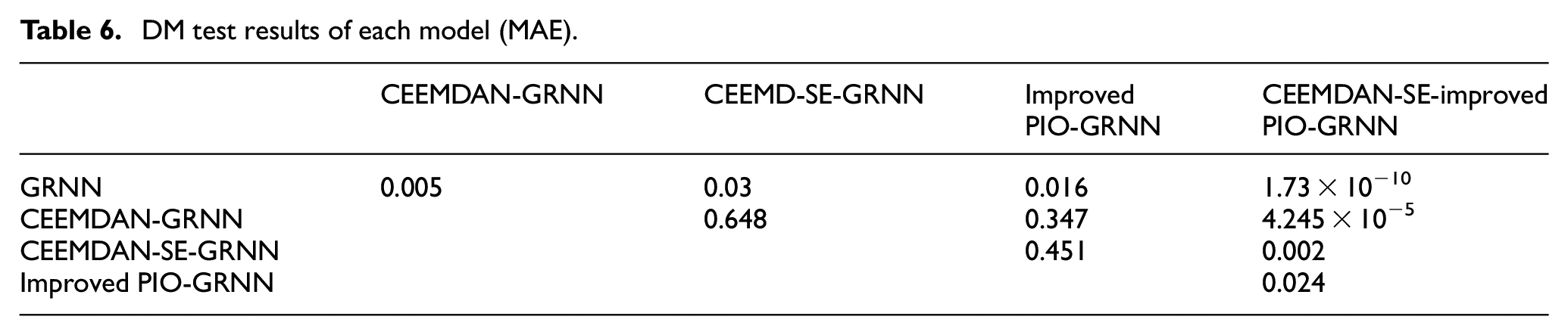
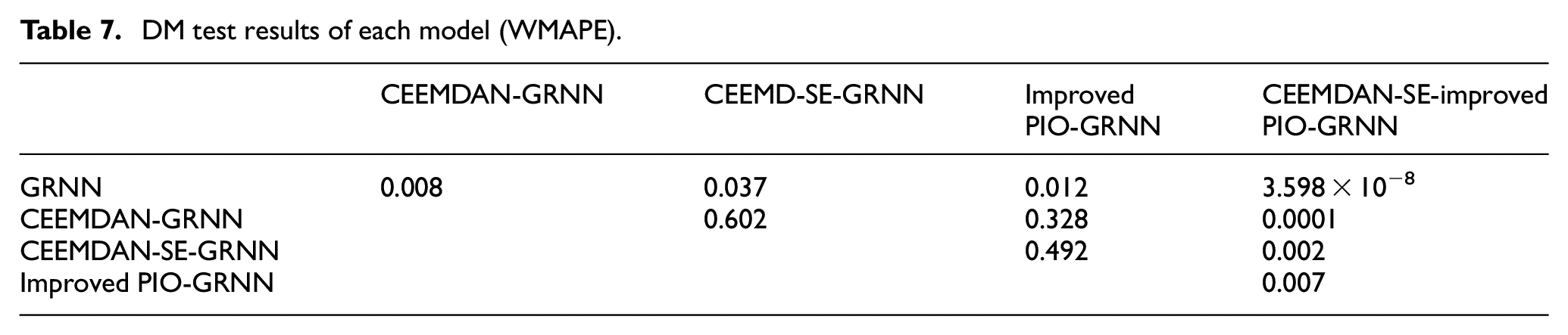
Compared with models GRNN, CEEMDAN-GRNN, CEEMDAN-SE GRNN, Improved PIO-GRNN, CEEMDAN-SE-GRNN, and CEEMDAN-SE-Improved PIO-GRNN, the DM test results based on MSE, MAE and WMAPE are calculated. The details are shown in Tables 5–7.
DM test results of each model (MSE).
DM test results of each model (MAE).
DM test results of each model (WMAPE).
As can be seen from Table 5, the DM test results in the MSE sense are as follows:
The model GRNN has the significant differences in predictive ability from CEEMDAN-GRNN, CEEMDAN-SE-GRNN, Improved PIO-GRNN, and CEEMDAN-SE- Improved PIO-GRNN, which indicates that the prediction ability of the latter four models is better than that of the GRNN model. Likewise, it can confidently indicate the prediction ability of CEEMDAN-SE-Improved PIO-GRNN is better than that of CEEMDAN-GRNN and CEEMDAN-SE-GRNN.
Correspondingly, the DM test value of CEEMDAN- GRNN and CEEMDAN-SE-GRNN in the model is 0.195, revealing that the prediction ability of CEEMDAN- SE-GRNN in the model is stronger than that of CEEMDAN-GRNN at the 20% significance level. Meanwhile, we can obtain the result that the difference in test result between the models CEEMDAN-GRNN and Improved PIO-GRNN is tiny. This result indicates that the original hypothesis with similar predictive ability cannot be obviously rejected, this may be due to some random factors. Likewise, for the model group CEEDMAN-SE-GRNN and Improved PIO-GRNN, and the model group Improved PIO-GRNN and CEEMDAN-SE-Improved PIO-GRNN, the same conclusion can be obtained.
It can be seen from Tables 6 and 7 that the DM test results in the meaning of MAE and WMAPE are as follows:
The predictive ability of the model GRNN is significantly different from that of the other four models, so it can be believed that the predictive ability of the other four models is indeed superior to GRNN. The significantly difference in predictive ability between CEEMDAN-GRNN and CEEMDAN-SE-Improved PIO-GRNN indicates the prediction ability of the latter is better than that of the former. Likewise, it also can confidently indicate the prediction ability of CEEMDAN-SE-Improved PIO-GRNN is better than that of CEEMD-SE-GRNN and Improved PIO-GRNN.
The difference in predictive ability between the models CEEMDAN-GRNN and CEEMDAN-SE-GRNN is tiny. This may be caused by random factors. Likewise, for the model group CEEMDAN-GRNN and Improved PIO-GRNN, and the model group CEEMDAN-SE-GRNN and Improved PIO-GRNN, the same conclusion can be obtained.
Combining Figures 11 and 12, Table 4 and DM test results, the fitting effect of CEEMDAN-GRNN prediction curve is better than that of GRNN. The MSE, MAE and WMAPE of CEEMDAN-GRNN are respectively 0.3609, 0.1512, and 3.8901% lower than that of GRNN, and the prediction ability difference is significant, which indicates that CEEMDAN decomposition can effectively reduce the interaction effect between various frequency components, thereby effectively improving the prediction accuracy. Hence, the variation trend of wind speed time sequences can be more well traced by this model.
The fitting degree and accuracy of prediction curve for CEEMDAN-SE-GRNN model are close to that of CEEMDAN-GRNN model. As revealed in the Table 4, MSE, MAE, and WMAPE of CEEMDAN-SE-GRNN model are separately decreased by 0.0586, 0.012, and 0.3084% compared with CEEMDAN-GRNN model. Results in the MSE meaning, it indicates that the prediction ability of CEEMDAN-SE-GRNN is stronger than that of CEEMDAN-GRNN at the 20% significant level. The reason is that the superposition of the error values for a single IMF is decreased within prediction procedure of CEEMDAN-SE-GRNN model. Therefore, the accuracy for the prediction is improved.
However, it is prone to be trapped in local optimum at several extremum points. Hence, the smoothing factor of GRNN is strengthened by applying the improved PIO. As displayed in Figure 12, Improved PIO-GRNN model has better effect of curve fitting than that of GRNN. Specifically, MSE, MAE, WMAPE are respectively decreased by 0.5095, 0.2006, and 5.1591%. And the DM test results show that there is a significant difference in their predictive ability. Therefore, the prediction effect of PIO-GRNN model is better than that of GRNN model.
The fitting effect of prediction curve for CEEMDAN-SE Improved PIO-GRNN is the best, and it can well forecast at wave crest and wave trough. Moreover, compared with the single prediction model, the prediction errors of MSE, MAE and WMAPE decreased by 0.6222, 0.3334, and 8.5766%, respectively. And the DM test results show that there is a significant difference in their predictive ability. It well illustrates that the prediction effect of the model proposed in this paper is better.
Conclusion
For the issue of intense fluctuation for wind speed time sequences, a short-term wind speed forecast method on account of CEEMDAN-SE-Improved PIO-GRNN model is proposed in this paper. The following are the conclusions.
Firstly, reducing the complexity of the wind speed sequences through decomposing these into a series of modes with different frequency bands by CEEMDAN. Then, merging the sequences with similar complexity into new sequences with the method SE. Moreover, separately establishing the new models for new sequences to implement the prediction. Consequently, both of prediction accuracy and arithmetic speed are effectively optimized.
To optimize the model’s forecast precision, the parameters of the Improved PIO algorithm are optimized by using improved the PIO. Firstly, optimizing the PIO algorithm by orthogonally designing the initial population so that the pigeons are distributed as evenly as possible in the whole space and the searching results are more accurate; Then, a dynamic adaptive geomagnetic operator is applied to keep the algorithm away from the local optimum.
The results of simulation experiments indicate that the forecast effect of the proposed model in this paper is relatively great.
Footnotes
Appendix
Notation
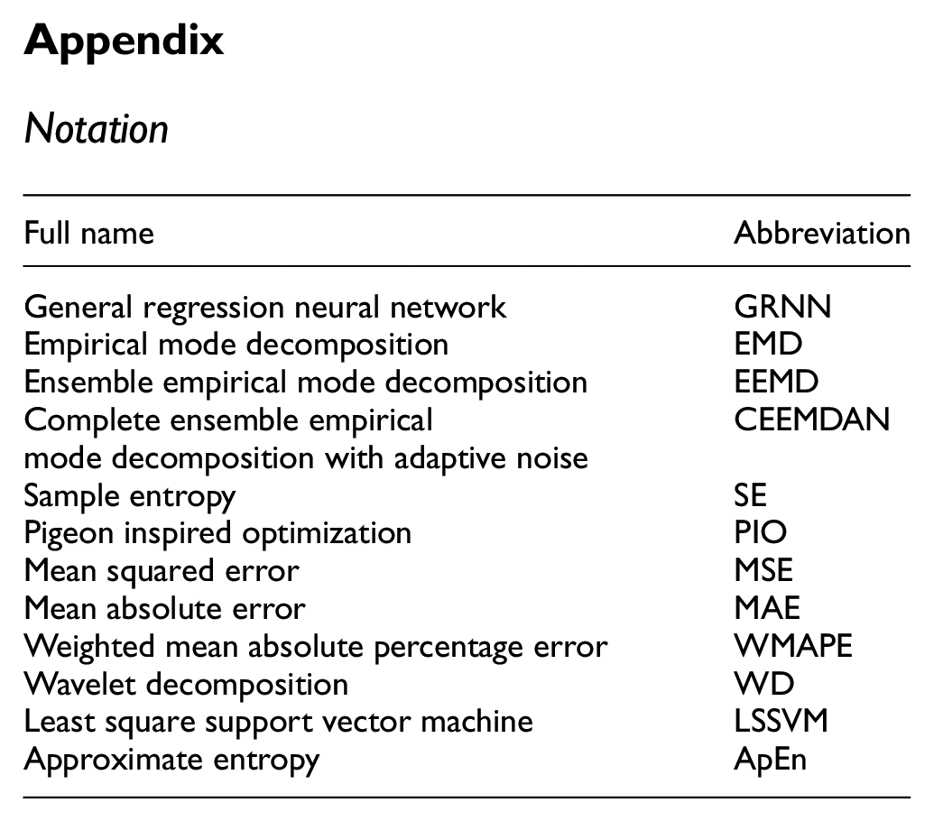
| Full name | Abbreviation |
|---|---|
| General regression neural network | GRNN |
| Empirical mode decomposition | EMD |
| Ensemble empirical mode decomposition | EEMD |
| Complete ensemble empirical mode decomposition with adaptive noise | CEEMDAN |
| Sample entropy | SE |
| Pigeon inspired optimization | PIO |
| Mean squared error | MSE |
| Mean absolute error | MAE |
| Weighted mean absolute percentage error | WMAPE |
| Wavelet decomposition | WD |
| Least square support vector machine | LSSVM |
| Approximate entropy | ApEn |
Declaration of conflicting interests
The author(s) declared no potential conflicts of interest with respect to the research, authorship, and/or publication of this article.
Funding
The author(s) disclosed receipt of the following financial support for the research, authorship, and/or publication of this article: This research was funded by Shanghai Science and Technology Commission scientific research project “Research on real-time simulation of grid-connected test platform and certification test technology for high-power wind turbines”, grant number “17DZ1201200”.