Sage Journals: Discover world-class research

Abstract

As a clean energy engine, the gas turbine is widely used for the generation of the power plant and the propulsion of the warship. Its control is becoming more and more challenging for the reason that internal coupling exists and the load command changes frequently and extensively. However, advanced controllers are difficult to implement on the distributed control system and conventional proportional–integral–derivative controllers are unable to handle with aforementioned challenges. To solve this problem, this article designs a decentralized active disturbance rejection control for the power and exhaust temperature of the gas turbine. Simulation results illustrate that the decentralized active disturbance rejection control is able to obtain satisfactory tracking and disturbance rejection performance with strong robustness. Eventually, a numerical simulation is carried out which shows advantages of active disturbance rejection control in the control of power and exhaust temperature when the gas turbine is under variable working condition. This successful application of decentralized active disturbance rejection control to the gas turbine indicates its promising prospect of field tests in future power industry with increasing demand on integrating more renewable energy into the grid.

Keywords

Gas turbine active disturbance rejection control power control exhaust temperature control variable working condition operation

Introduction

The gas turbine (GT) is a typical internal combustion engine which is widely used for the generation of power plants and the propulsion of warships. It consists of the combustion chamber, the compressor, and turbines. When a GT is in its common operating mode, the working medium inside it completes a thermodynamic cycle which can be regarded as a simple Brayton cycle. According to their structures, GTs are generally classified by three categories: the heavy-duty gas turbine (HDGT), the light-duty gas turbine (LDGT), and the micro gas turbine (MGT). Because of its long service life and high efficiency, the HDGT is mostly applied in modern industry.

In a generation system of power plant with the GT, the shaft of the generator and the output shaft of the prime motor are connected. As a result, the generator and the GT are driven by the same shaft which converts the mechanical energy to electricity. The output power of the GT is of significance for the reason that it decides the electricity generation of the power plant. The power demand is varying with the load command which requires the output power of the GT should track the set point actively when the working condition is changing. Moreover, the inlet temperature of the turbine is critical for the control of a GT but it is difficult to measure. As a result, researchers focus on the control of exhaust temperature in turn.

In the past decades, there were previous studies proposed for multivariable control of the GT. Model predictive controller (MPC) was applied to the control of shaft speed and exhaust temperature for a GT power plant. Compared with the SpeedTronic control system, it was able to maintain the rotor speed more accurate using simultaneous exhaust temperature control.¹ In addition, a H_∞ robust controller is designed for an identified model of MONTAZER GHAEM power plant GT (GE9001E).² Simulation results show the robust controller has the better performance on the control of the rotor speed and the exhaust temperature than the proportional–integral–derivative (PID) controller when the demand power is varying.

However, in terms of field applications, these advanced control strategies are challenging to implement on the distributed control system (DCS) of an HDGT. Nowadays, conventional PID controllers are commonly used in the control system of HDGT, but their hysteretic regulating characteristics limit the response speed of the system and the ability of rejection of possible disturbances such as the sharp increase of valve opening and the fluctuation of air temperature.³ Therefore, it is of necessity to find a simple controller which is able to obtain better control performance than PID.

Active disturbance rejection control (ADRC), proposed by Chinese scholar J Han,⁴ is considered as the successor of PID in modern industry. The core idea of ADRC is that uncertainties, external disturbances, and the modeling errors are all integrated as an extended state which is estimated and compensated by the extended state observer (ESO).⁵ Compared with the conventional PID controller, ADRC inherits its advantages and has less dependency on the accurate mathematical model of the process. However, the nonlinear ADRC is unavailable for the configuration of DCS. To solve this problem, Z Gao⁶ simplified ADRC into linear form and standardized the tuning procedure of parameters of linear ADRC (LADRC) on the basis of the bandwidth-parameterization method. This simplification enabled ADRC to be applied in industrial systems such as superheated steam temperature,^7,8 gyroscopes,⁹ gasifiers,¹⁰ hydroturbine speed,¹¹ the secondary air flow,¹² fuel-cell temperature,¹³ DC–DC buck converter,¹⁴ chemical system,¹⁵ and waste heat recovery system.¹⁶

The rest of this paper is organized as follows: In the next section, the mechanism model and transfer function models are established to describe the multivariable process of the power and exhaust temperature of the GT. Based on the models established in section “2,” control difficulties such as strong nonlinearity and coupling are analyzed in section “Control difficulties analysis.” Section “Design of the control systems” briefly introduces the theory of LADRC and followed by the design of comparative control strategies including decentralized proportional–integral (PI) and inverted decoupling PI (IDPI) controller. In section “Simulation results,” the decentralized LADRC is applied to the multivariable system of the GT by numerical simulations. Eventually, concluding remarks are offered in the last section.

The model of the GT

Figure 1 shows the configuration of a GT. The pressure, the temperature, the flow rate, and the enthalpy are defined as P, T, G, and H, respectively. Several assumptions are proposed in order to simplify the modeling of the GT:

Ignore the thermal inertia of all components and the combustion delay.

Ignore the influence of altitude.

The flow of gas in the GT is regarded as one-dimensional flow.

The working medium is considered as ideal gas.

Compression and expansion of gas are approximated as adiabatic processes.

Constant thermo-physical properties are assumed such as the air constant (γ_air), the gas constant (γ_gas), and lower heating value of the fuel (LHV).

All volumes are constant.

Figure 1.

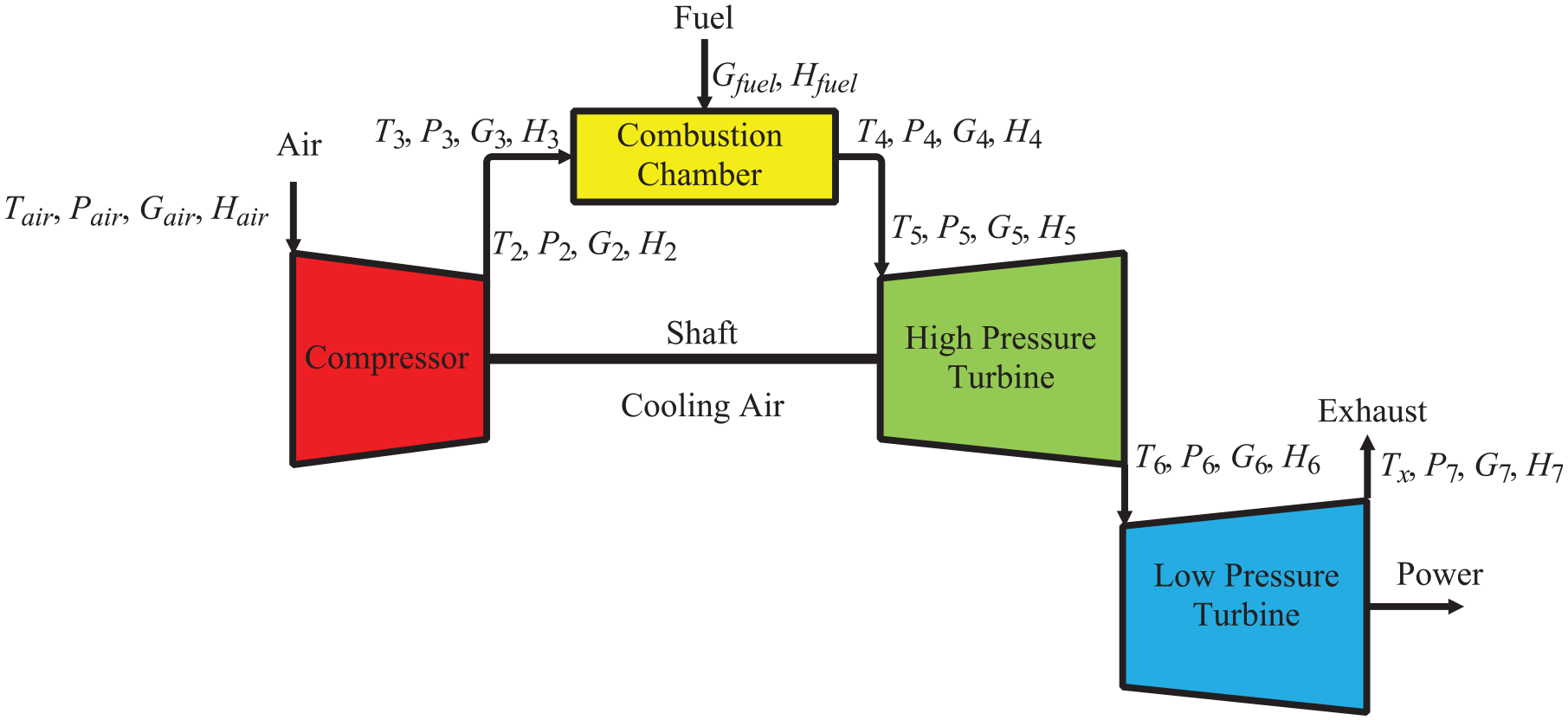
The configuration of the gas turbine.

Moreover, since the working medium is regarded as the ideal gas, its enthalpy is the monotropic function of the temperature.

Mechanism model

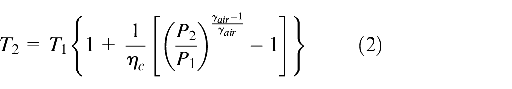
The compressor map is two-dimensional (2D) which can evaluate the efficiency (η_c) and the corrected mass flow rate (G_c) of compressor as follows

(\frac{\sqrt{T_{1}}}{P_{1}}, \frac{n}{\sqrt{T_{1}}}) \overset{compressor map}{\to} (G_{c}, η_{c})

(1)

T_{2} = T_{1} {1 + \frac{1}{η_{c}} [{(\frac{P_{2}}{P_{1}})}^{\frac{γ_{air} - 1}{γ_{air}}} - 1]}

(2)

P_{c} = G_{c} (H_{2} - H_{1})

(3)

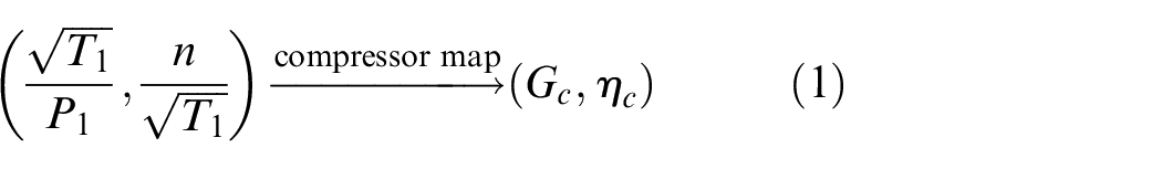
where n represents the shaft speed and P_c refers to the power of the compressor.

In Figure 1, G_fuel and H_fuel are defined as the flow rate and enthalpy of the fuel, respectively. The pressure of the gas (P₄) and the heat balance in the chamber are depicted as follows

P_{4} = σ_{cb} P_{3}

(4)

G_{4} H_{4} = G_{3} H_{3} + G_{fuel} (H_{fuel} + η_{cb} LHV)

(5)

where σ_cb represents the combustion pressure recovery factor. η_cb is denoted as the efficiency of combustion.

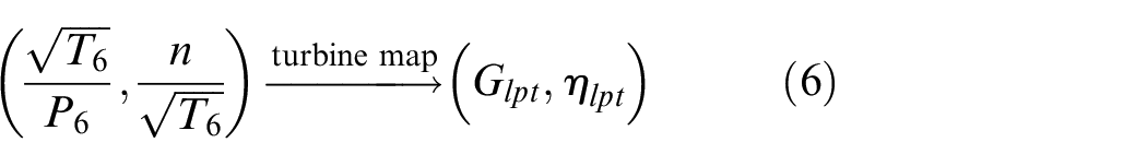
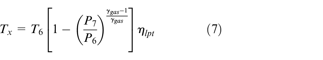
In this paper, the power and the exhaust temperature are regarded as the controlled variables of the GT. Therefore, in this subsection, the low-pressure turbine (LPT) is taken as an example. The efficiency (η_lpt) and the corrected mass flow rate (G_lpt) of LPT are able to be obtained by the 2D turbine map. According to Figure 1, the power (P_t) and the exhaust temperature (T_x) are depicted as

(\frac{\sqrt{T_{6}}}{P_{6}}, \frac{n}{\sqrt{T_{6}}}) \overset{turbine map}{\to} (G_{lpt}, η_{lpt})

(6)

T_{x} = T_{6} [1 - {(\frac{P_{7}}{P_{6}})}^{\frac{γ_{gas} - 1}{γ_{gas}}}] η_{lpt}

(7)

P_{t} = G_{6} (H_{6} - H_{7})

(8)

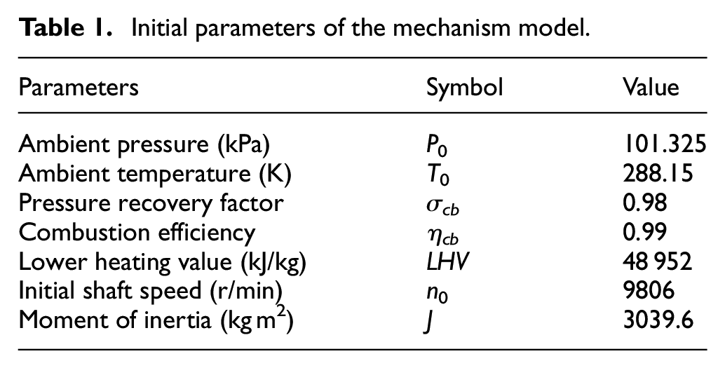
In addition, several initial parameters are set as shown in Table 1 to complete the iterative calculations in the model.

Table 1.

Initial parameters of the mechanism model.

Parameters	Symbol	Value
Ambient pressure (kPa)	P ₀	101.325
Ambient temperature (K)	T ₀	288.15
Pressure recovery factor	σ_cb	0.98
Combustion efficiency	η_cb	0.99
Lower heating value (kJ/kg)	LHV	48 952
Initial shaft speed (r/min)	n ₀	9806
Moment of inertia (kg m²)	J	3039.6

Transfer function model

For the simple analysis of the GT, its mechanism model is identified as the 2 × 2 transfer function matrix as follow

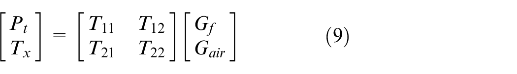
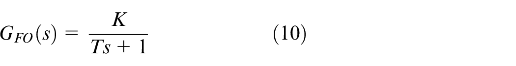
[\begin{matrix} P_{t} \\ T_{x} \end{matrix}] = [\begin{matrix} T_{11} & T_{12} \\ T_{21} & T_{22} \end{matrix}] [\begin{matrix} G_{f} \\ G_{air} \end{matrix}]

(9)

where T₁₁ and T₂₁ are identified as first-order (FO) transfer functions which are depicted as equation (10); T₁₂ and T₂₂ are identified as second-order transfer functions plus zero (SOPZ) which are depicted as equation (11)

G_{FO} (s) = \frac{K}{Ts + 1}

(10)

G_{SOPZ} (s) = \frac{K (1 - ps)}{(T_{1} s + 1) (T_{2} s + 1)}

(11)

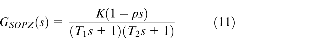
Besides, G_air is denoted as the flow rate of air. To analyze the characteristics and control difficulties of the GT, we identify the transfer function matrix under four different working conditions including 100% load, 76% load, 60% load, 51% load, and 31% load. Table 2 lists these steady-state working conditions.

Table 2.

Steady-state working conditions.

Load (%)	G_fuel (kg/s)	G_air (kg/s)	P_t (kW)	T_x (°C)
31	0.772	50.321	11,639.166	472.155
51	1.043	61.983	15,888.511	501.675
60	1.203	68.480	18,688.209	513.257
76	1.464	78.375	23,808.253	525.976
100	1.795	86.300	30,330.191	556.412

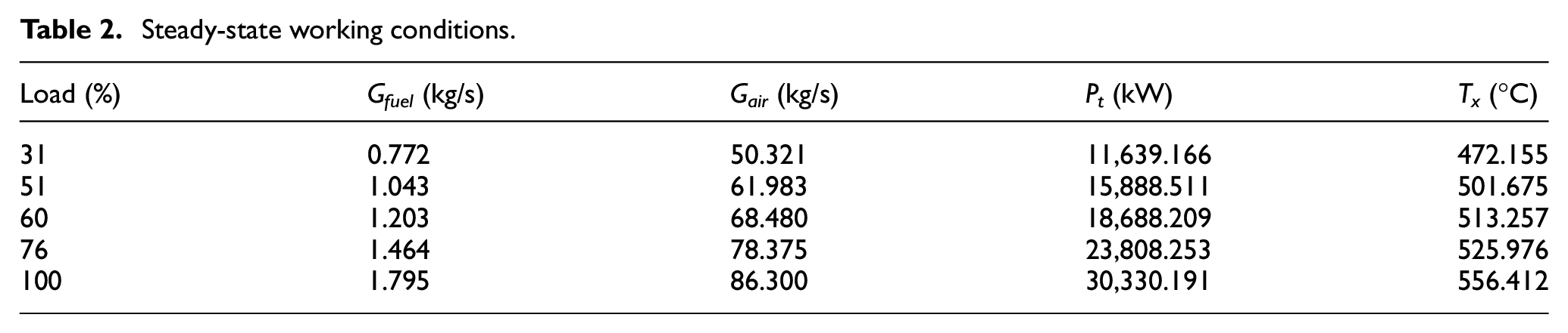
Based on Table 2, transfer functions of different working conditions are identified as equation (12)–(16).

T_{100 %} = [\begin{matrix} \frac{13047.070}{0.133 s + 1} & \frac{303.262 (5.490 s + 1)}{(0.697 s + 1) (0.870 s + 1)} \\ \frac{227.351}{0.242 s + 1} & \frac{- 6.631 (1 - 21.452 s)}{(1.049 s + 1) (1.035 s + 1)} \end{matrix}]

(12)

T_{76 %} = [\begin{matrix} \frac{12445.155}{0.213 s + 1} & \frac{262.373 (5.791 s + 1)}{(0.751 s + 1) (0.927 s + 1)} \\ \frac{275.885}{0.329 s + 1} & \frac{- 6.906 (1 - 22.221 s)}{(1.005 s + 1) (0.979 s + 1)} \end{matrix}]

(13)

T_{60 %} = [\begin{matrix} \frac{11818.950}{0.213 s + 1} & \frac{177.346 (6.511 s + 1)}{(0.874 s + 1) (0.845 s + 1)} \\ \frac{338.420}{0.395 s + 1} & \frac{- 7.060 (1 - 31.776 s)}{(1.145 s + 1) (1.505 s + 1)} \end{matrix}]

(14)

T_{51 %} = [\begin{matrix} \frac{11234.165}{0.253 s + 1} & \frac{53.017 (37.812 s + 1)}{(1.193 s + 1) (1.219 s + 1)} \\ \frac{379.315}{0.375 s + 1} & \frac{- 6.457 (1 - 25.239 s)}{(1.005 s + 1) (0.979 s + 1)} \end{matrix}]

(15)

T_{31 %} = [\begin{matrix} \frac{11180.315}{0.327 s + 1} & \frac{250.507 (0.249 s + 1)}{(0.270 s + 1) (0.860 s + 1)} \\ \frac{497.330}{0.475 s + 1} & \frac{- 10.534 (1 - 37.953 s)}{(2.820 s + 1) (0.911 s + 1)} \end{matrix}]

(16)

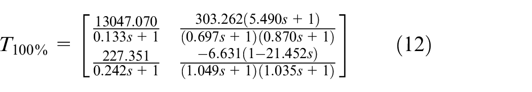
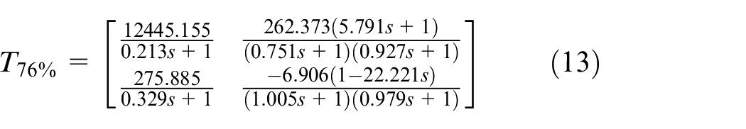
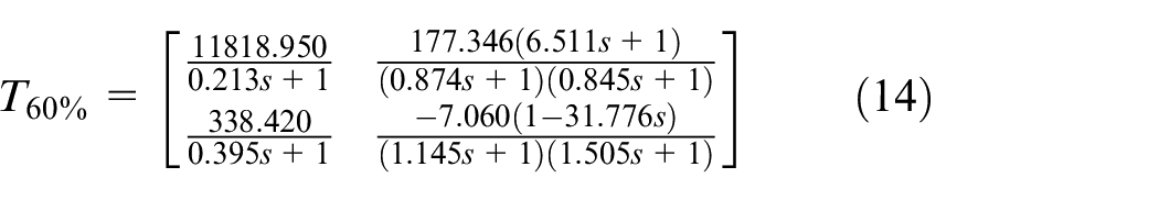
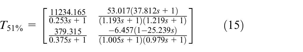
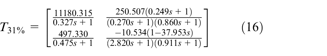
Note that control difficulties of the GT such as strong nonlinearity and coupling are all analyzed based on transfer functions of aforementioned working conditions.

Control difficulties analysis

Components of the GT are connected by pipelines, which may form strong nonlinearities. As a result, the dynamic characteristics of GT vary significantly at different working conditions. Figure 2 shows open-loop responses of the system at operating points mentioned in subsection “Transfer function model.”N is denoted as the load. In this paper, the nonlinearity of the multivariable control system is evaluated by gap metric, which is regarded as a measurement of the distance between two linear time-invariant (LTI) systems.^17,18

Figure 2.

Open-loop responses at different working conditions.

The gap between two systems is denoted as δ which can be depicted as

δ (G_{1}, G_{2}) = max [\vec{δ} (G_{1}, G_{2}), \vec{δ} (G_{2}, G_{1})]

(17)

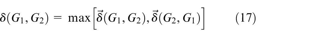
where G₁ and G₂ are transfer functions linearized around two different working conditions. $\vec{δ} (G_{1}, G_{2})$ represents the direct gap which is defined as

\vec{δ} (G_{1}, G_{2}) = inf_{A \in H_{\infty}} ‖ [\begin{matrix} P_{1} \\ Q_{1} \end{matrix}] - [\begin{matrix} P_{2} \\ Q_{2} \end{matrix}] A ‖

(18)

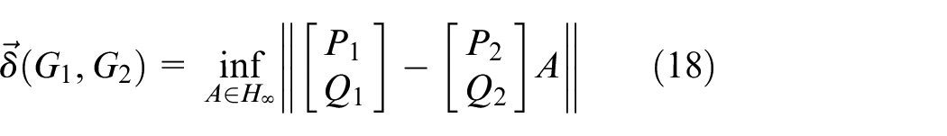
where G₁ = Q₁P₁⁻¹ and G₂ = Q₂P₂⁻¹. A is a matrix parameter which has H_∞ form. The gap is restricted as

0 \leq \vec{δ} (G_{1}, G_{2}) \leq 1

(19)

The high value of gap means strong nonlinearity and vice versa. In this section, G₁ is set as the nominal transfer function which is linearized around 31% load. The gap is plotted as Figure 3.

Figure 3.

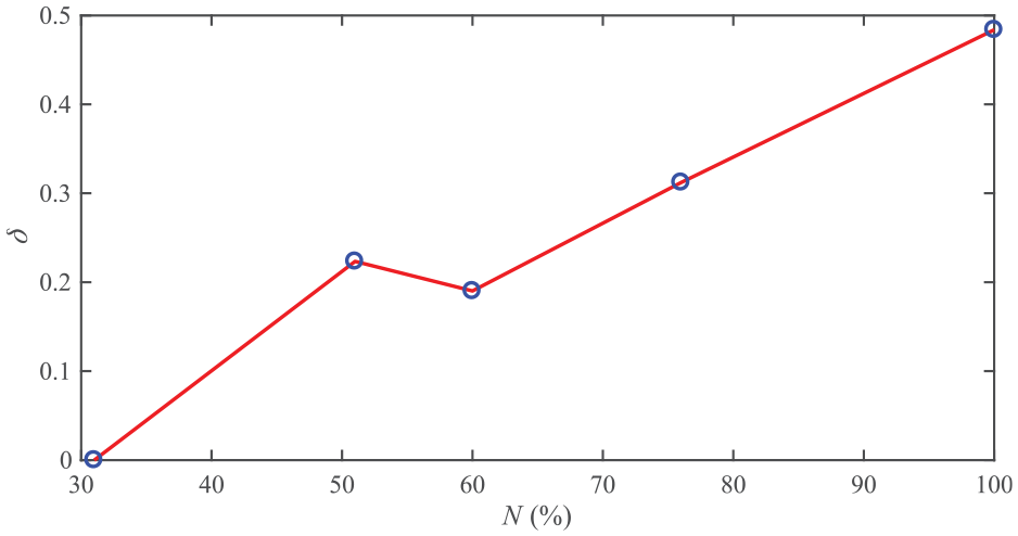
Gap measurement of different working conditions.

From Figure 3, it is evident that the gap is big when the load is high. Since the big gap represents the significant difference between two systems, it is easy to understand that the transfer function of 31% load is irrelevant to those of other working conditions. As a result, the dynamic characteristics at 31% load is different with those at 51% load, 60% load, 76% load, and 100% load. In addition, from equations (12)–(16), gains and time constants of each transfer function in two-input two-output (TITO) system at different operating points are totally different. Therefore, the dynamic characteristics of the TITO system change significantly with the working condition. Besides, the control strategy designed for this system should be robust enough in order to obtain satisfactory control performance at off-design operating points.

Moreover, in a multivariable control system, the coupling refers to the interactions between controlled variables and manipulated variables. According to the coupling degree, the decoupling technology is considered to be nor not to be applied to eliminate the interaction. The relative gain array (RGA) is a matrix to evaluate the coupling degree in a TITO system. Figure 4 illustrates the frequency-dependent RGA of different working conditions.

Figure 4.

Frequency-dependent RGA for the gas turbine under all working conditions.

According to Figure 4, it is obvious that the coupling degree in this TITO system is low, which means that the interaction between controlled variables and manipulated variables are weak. Therefore, the decentralized control structure is able to be applied to this TITO system.

Design of the control systems

Structures of the multivariable control system

Decentralized control and decoupling control are main control structures for a TITO system. Besides, as for decoupling control, it consists of inverted decoupling control, simple decoupling control and ideal decoupling control. In this paper, decentralized control structure and inverted decoupling structure are applied to the TITO system depicted as equation (9).

In Figure 5, the power demand and the set point of exhaust temperature change with the load command. As mentioned in section 3, the decoupling degree in this TITO system is strong so that inverted decouplers may be applied to it. Besides, d_fuel, d_air, and d_tamb are denoted as disturbances caused by the flow rate of fuel, the flow rate of air, and the ambient temperature, respectively. Figure 6 shows the block diagram of the inverted decoupling control.

Figure 5.

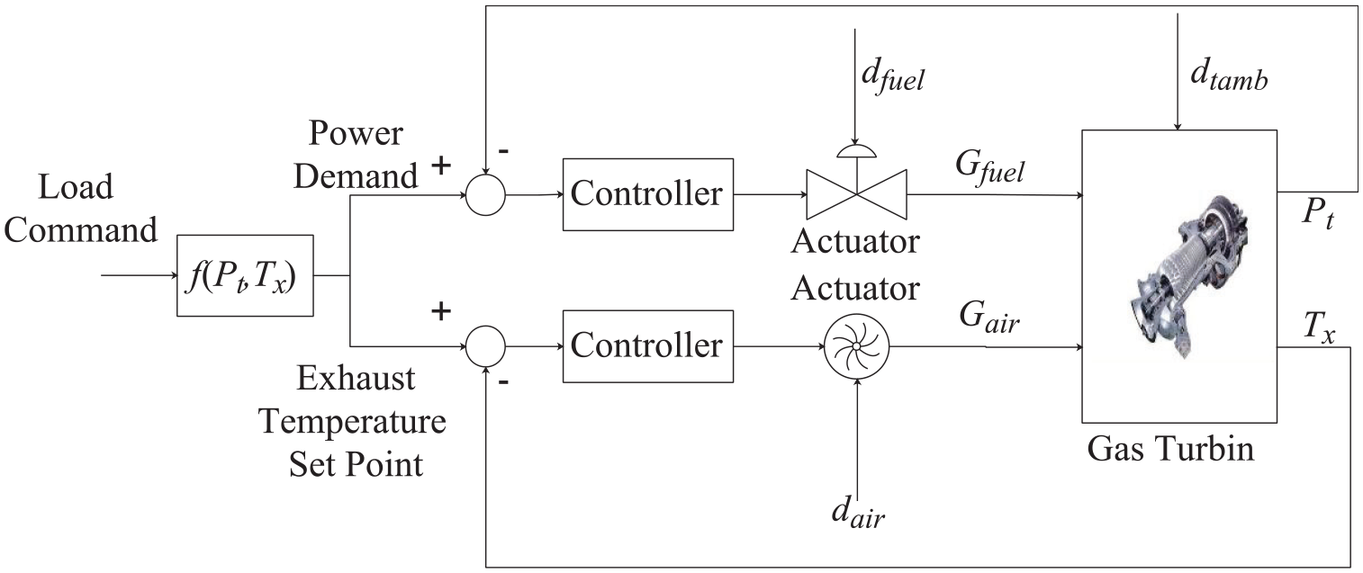
Block diagram of decentralized control.

Figure 6.

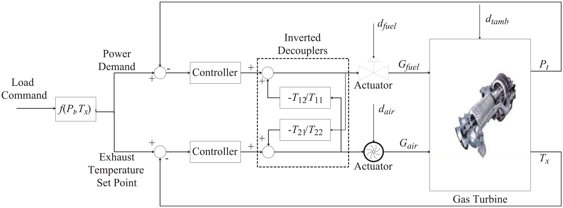
Block diagram of inverted decoupling control.

where T₁₁, T₁₂, T₂₁, and T₂₂ have been defined in equation (9).

ADRC

In this paper, we apply the FO LADRC to the GT control system. As for LADRC, it consists of two parts: the state feedback control law (SFCL) and the ESO. Suppose that the controlled object is able to be regarded as a general FO system

\overset{\cdot}{y} = g (t, y, \overset{\cdot\cdot}{y}, \overset{\dots}{y}, \dots, d) + bu

(20)

where g is the synthesis of high-order dynamics, modeling error, and external disturbances of the system. u and y are denoted as the input and output, respectively. b refers to the critical gain whose value may be uncertain for a process.¹⁹ Consequently, equation (17) can be rewritten as

\overset{\cdot}{y} = f + b_{0} u

(21)

where b₀ is the estimation of b and f is defined as the total disturbance of the system which equals g + (b – b₀). Let the state vector of the FO system x = [x₁x₂]^T = [y f]^T, where x₂ is considered as the extended state. Therefore, the expressions of the general FO system is able to be depicted as

{\begin{matrix} {\overset{\cdot}{x}}_{1} = x_{2} + b_{0} u \\ {\overset{\cdot}{x}}_{2} = \overset{\cdot}{f} \\ y = x_{1} \end{matrix}

(22)

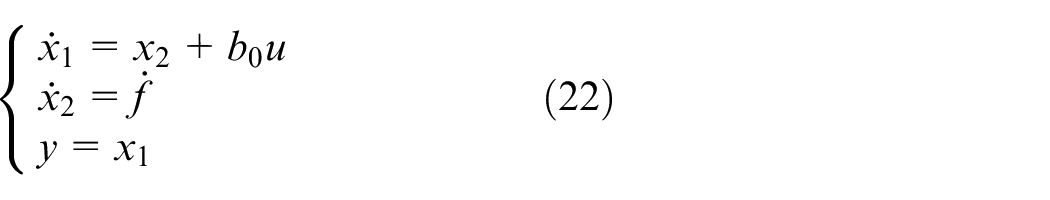
The ESO is designed for the system as

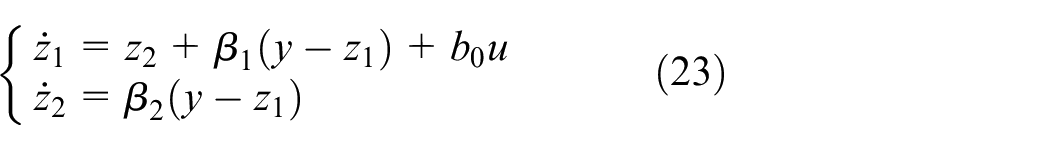
{\begin{matrix} {\dot{z}}_{1} = z_{2} + β_{1} (y - z_{1}) + b_{0} u \\ {\dot{z}}_{2} = β_{2} (y - z_{1}) \end{matrix}

(23)

where β₁ and β₂ are gains of ESO.

The SFCL is designed as

u = \frac{k_{p} (r - z_{1}) - z_{2}}{b_{0}}

(24)

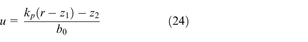
where r is denoted as the set point and k_p is the tunable parameter of the controller. Z Gao⁶ proposed a tuning method of the FO LADRC based on bandwidth-parameterization in order to simplify its tuning procedure.

If β₁ and β₂ are chosen appropriately, z = [z₁z₂]^T is able to track x accurately.²⁰ Therefore, the process is reduced to a unit FO integrator. Equation (18) can be derived as

\overset{\cdot}{y} + k_{p} y = k_{p} r

(25)

The closed-loop characteristic polynomial G(s) enables to be written as

G (s) = s + k_{p} = s + ω_{c}

(26)

where ω_c is denoted as the bandwidth of the feedback control system. The characteristic polynomial of the ESO is able to be depicted as

s^{2} + β_{1} s + β_{2} = {(s + ω_{o})}^{2}

(27)

where ω_o is denoted as the bandwidth of ESO. Consequently, parameters of the FO LADRC can be summarized as

k_{p} = ω_{c}, β_{1} = 2 ω_{o}, β_{2} = {ω_{o}}^{2}

(28)

Note that b₀ is regarded as a tunable parameter of the FO LADRC as well. Figure 7 shows the block diagram of FO LADRC.

Figure 7.

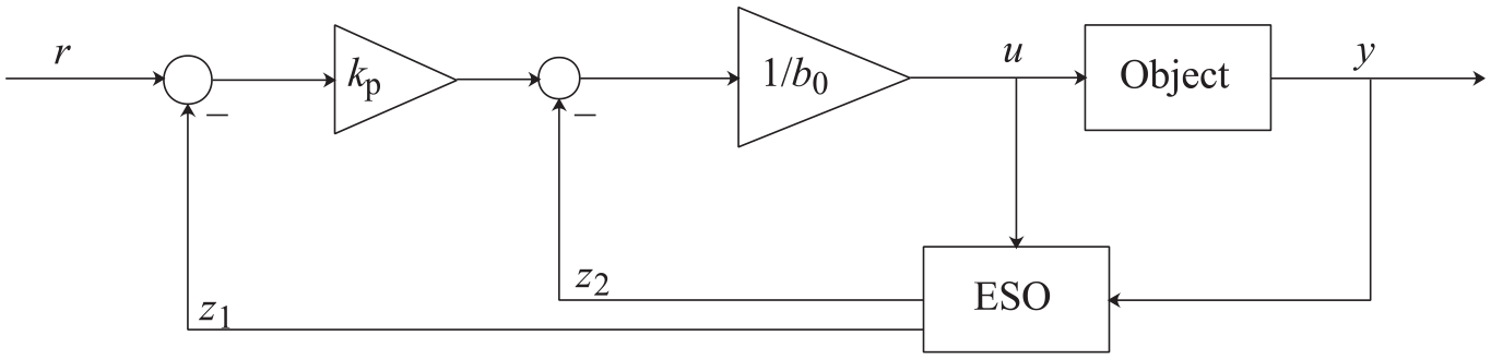
The block diagram of first-order ADRC.

It has been proven that the decentralized LADRC has the ability to decouple.²¹ As a result, the LADRC is designed for the TITO system of GT based on the decentralized control structure.

Following rules are able to be regarded as the guidance of ADRC tuning:

With the increase of ω_o, the ability of ESO to estimate and compensate disturbances will enhance. Note that ω_o is unable to be augmented infinitely for the reason that the noise sensitivity of ESO will increase simultaneously. As a result, ω_o should be gradually augmented from a small value until the output has no obvious change. Generally, it is recommended to be set as 3–5 ω_c.⁶

A larger ω_c or a smaller b₀ means faster output response. However, with the increase of ω_c or the decrease of b₀, the overshoot will be larger and the oscillation will be fiercer. Actually, b₀ should not be far from b in order to obtain satisfactory control performance.

Comparative control strategies

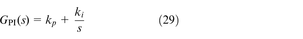
In this paper, the decentralized PI and IDPI are set as comparative control strategies. The transfer function of PI controller is depicted as

G_{PI} (s) = k_{p} + \frac{k_{i}}{s}

(29)

All parameters of PI controllers are tuned based on Skogastad Internal Model Control (SIMC).²² Besides, the inverted decouplers are derived under the same working condition which are depicted as

D_{1} (s) = - \frac{T_{12} (s)}{T_{11} (s)} = - \frac{0.023 (5.490 s + 1) (0.133 s + 1)}{(0.697 s + 1) (0.870 s + 1)}

(30)

D_{2} (s) = - \frac{T_{21} (s)}{T_{22} (s)} = \frac{34.286 (1.049 s + 1) (1.035 s + 1)}{(0.242 s + 1) (1 - 21.452 s)}

(31)

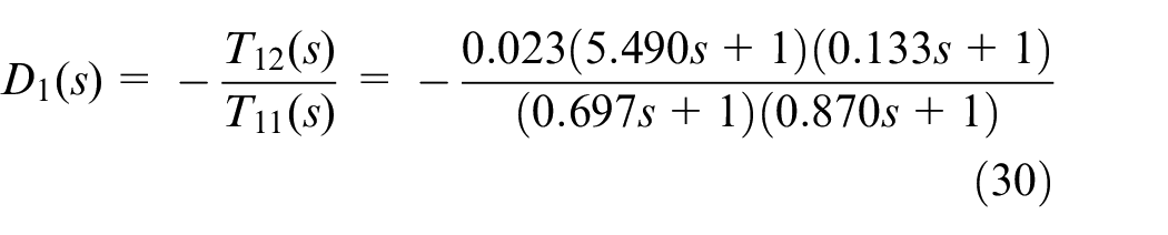
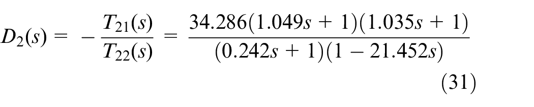
where D₁(s) and D₂(s) are denoted as decouplers as shown in Figure 5. Table 3 illustrates the parameters of different control strategies.

Table 3.

Parameters of different control strategies.

Controlstrategies	Loop	Parameters
PI	Loop 1	k_p ₁ = 3.832 × 10⁵, k_i₁ = 2.881 × 10⁴
PI	Loop 2	k_p ₂ = −0.0167, k_i₂ = −0.504
IDPI	Loop 1	k_p ₁ = 3.066 × 10⁵, k_i₁ = 2.305 × 10⁴
IDPI	Loop 2	k_p ₂ = −0.101, k_i₂ = −0.704
ADRC	Loop 1	ω_c ₁ = 4, ω_o₁ = 16, b₀₁ = 7.5244 × 10⁴
ADRC	Loop 2	ω_c ₂ = 75, ω_o₂ = 100, b₀₂ = −4 × 10³

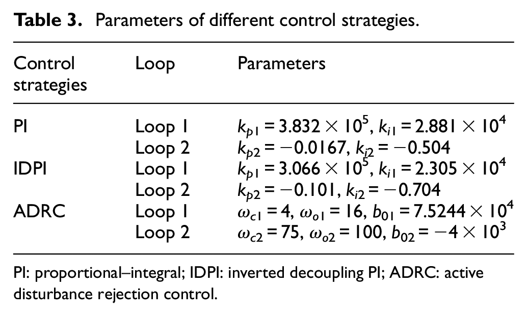
PI: proportional–integral; IDPI: inverted decoupling PI; ADRC: active disturbance rejection control.

In Table 3, parameters with subscribe “1” are denoted as the parameters of the control strategy of the G_fuel–P_t loop (Loop 1), while those with subscribe “2” are denoted as the parameters of the control strategy of the G_air–T_x loop (Loop 2).

Simulation results

Reference tracking

In this subsection, dynamic indices such as the overshoot or undershoot (σ) and the settling time (T_s) are selected to evaluate the tracking performance of a controller. The settling time is recorded based on 2% principle. Moreover, the integral absolute error (IAE) is a comprehensive index to measure the dynamic performance of the control strategy. IAE is depicted as

IAE = \int_{o}^{T} | e (t) | dt

(32)

where e(t) is defined as the tracking error of the controller variable. IAE tends to produce responses with less sustained oscillation.²³ IAE_sp refers to the IAE of tracking in this paper.

The full working condition is regarded as the nominal operating point for the reason that all control strategies are designed under 100% load. In this subsection, set points are changing under at the nominal operating point in order to evaluate the tracking performance of different control strategies. The set point of power is changing from 30,330.191 kW to 27,613.167 kW, while that of exhaust temperature is changing from 556.413 °C to 543.764°C. Figures 8 and 9 illustrate the tracking performance of power and exhaust temperature with different control strategies. In addition, Figure 10 shows variations of manipulated variables of the TITO system.

Figure 8.

The tracking performance of power.

Figure 9.

The tracking performance of exhaust temperature.

Figure 10.

Variations of manipulated variables.

From Figure 8, as for the control of power, it is obvious that ADRC has the smallest undershoot compared with PI and IDPI; from Figure 9, in terms of the control of exhaust temperature, IDPI is able to track the set point more sufficiently than PI and ADRC.

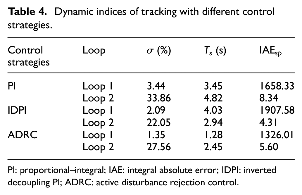
Table 4 shows the dynamic indices of tracking with different control strategies. In this section, the undershoot, the settling time, and IAE_sp are recorded from 10 to 19 s.

Table 4.

Dynamic indices of tracking with different control strategies.

Control strategies	Loop	σ (%)	T_s (s)	IAE_sp
PI	Loop 1	3.44	3.45	1658.33
PI	Loop 2	33.86	4.82	8.34
IDPI	Loop 1	2.09	4.03	1907.58
IDPI	Loop 2	22.05	2.94	4.31
ADRC	Loop 1	1.35	1.28	1326.01
ADRC	Loop 2	27.56	2.45	5.60

PI: proportional–integral; IAE: integral absolute error; IDPI: inverted decoupling PI; ADRC: active disturbance rejection control.

We expect that outputs of the multivariable control system have the smallest overshoot or undershoot, the shortest settling time and the smallest IAE. According to Table 4, some remarks are given as follows:

In terms of Loop 1, ADRC has the smallest undershoot, the shortest settling time and the smallest IAE_sp.

As for Loop 2, IDPI has the smallest undershoot and IAE_sp. However, its settling time is a bit longer than ADRC. Although IDPI shows its advantages in tracking of exhaust temperature at the nominal operating point, its tracking performance is worse at off-design operating points which will be discussed in the following subsection.

Disturbance rejection

In the GT, various external disturbances which caused by the environment and fuel may greatly impact on dynamic performance of control strategies. Therefore, it is important to verify the disturbance rejection abilities. In this subsection, disturbances such as the sharp ascent or descent of the fuel flow rate (d_fuel), the fluctuation of ambient temperature (d_tamb), and the sudden ascent or descent of the air flow rate (d_air) are added to the GT. All these disturbances are produced under the nominal working condition, that is, 100% load. In order to evaluate the disturbance rejection performance of different control strategies, IAE is chosen as the dynamic index as well. Besides, IAE_ud1, IAE_ud2 and IAE_ud3 are denoted as the IAE of rejecting disturbances caused by fuel flow rate, the air flow disturbance, and the ambient temperature, respectively.

First, the control signal of the fuel valve is disturbed by other signals in the field so that the flow rate of fuel will step up. Therefore, suppose that d_fuel is a positive step signal whose amplitude is 0.2. It is added at 20 s. Figure 11 shows outputs with different control strategies under the disturbance of fuel flow rate.

Figure 11.

Rejection performance with different control strategies under the disturbance of fuel flow rate.

From Figure 11, it is obvious that outputs of ADRC are able to recover to set points faster than those of PI and IDPI. This means that ADRC can reject disturbances caused by the flow rate of fuel more effectively.

Second, the position of the inlet guide vane (IGV) may be perturbed by external signals which will lead to the sharp ascent or descent of the air flow rate. In this subsection, d_air is considered as a negative step signal whose amplitude is 2. It is added at 30 s. Figure 12 illustrates outputs with different control strategies under the disturbance of air flow rate.

Figure 12.

Rejection performance with different control strategies under the disturbance of air flow rate

According to Figure 12, it is evident that ADRC enables outputs to track the set point faster than PI and IDPI when the disturbance of air flow rate exists. Hence, ADRC has better rejection performance of disturbances caused by the flow rate of air than other comparative control strategies.

Third, during the operation of the GT, the ambient temperature is fluctuating which may influence the generation efficiency. Assume that d_tamb is a periodical signal. The ambient temperature starts to fluctuate at 50 s. Figure 13 shows outputs with different control strategies under the disturbance of ambient temperature.

Figure 13.

Rejection performance with different control strategies under the disturbance of ambient temperature.

Obviously, the power and exhaust temperature have the smallest fluctuating amplitudes under the periodical disturbance caused by the ambient temperature when ADRC is applied to the system. As a result, ADRC is able to reject the fluctuation of ambient temperature more effectively than PI and IDPI.

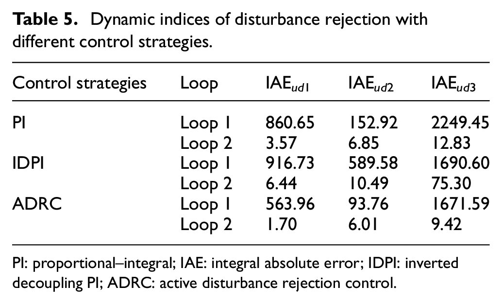
Finally, IAE_ud1, IAE_ud2 and IAE_ud3 are recorded in order to evaluate disturbance rejection performance of different control strategies. They are recorded from 19 to 23 s, 29 to 33 s, and 50 to 75 s, respectively. Table 4 shows dynamic indices of disturbance rejection with different control strategies.

According to Table 5, ADRC shows its advantages in disturbance rejection. Following are some remarks:

In terms of Loop 1, ADRC has the smaller IAE_ud1, IAE_ud2 and IAE_ud3 than other comparative control strategies.

As for Loop 2, the IAE_ud1, IAE_ud2, and IAE_ud3 of ADRC are smaller than those of other comparative control strategies.

Table 5.

Dynamic indices of disturbance rejection with different control strategies.

Control strategies	Loop	IAE_ud1	IAE_ud2	IAE_ud3
PI	Loop 1	860.65	152.92	2249.45
PI	Loop 2	3.57	6.85	12.83
IDPI	Loop 1	916.73	589.58	1690.60
IDPI	Loop 2	6.44	10.49	75.30
ADRC	Loop 1	563.96	93.76	1671.59
	Loop 2	1.70	6.01	9.42

PI: proportional–integral; IAE: integral absolute error; IDPI: inverted decoupling PI; ADRC: active disturbance rejection control.

Robustness test

From Figure 2, it is obvious that open-loop responses of power and exhaust temperature change significantly with the operating point. As a result, it is of importance that a controller is able to obtain satisfactory control performance when the load command is varying. A system is robust when it has acceptable changes in performance due to model changes or inaccuracies.¹⁷ Monte Carlo trial is an effective method to test the robustness of a controller. It is able to intuitively indicate the system with which controller will obtain strongest robustness and best dynamic performance.

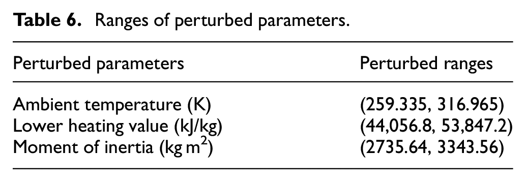
In this subsection, parameters such as the moment of inertia, lower heating value of the fuel, and the ambient temperature are perturbed within a range of ±10%. Ranges of these perturbed parameters are listed in Table 6.

Table 6.

Ranges of perturbed parameters.

Perturbed parameters	Perturbed ranges
Ambient temperature (K)	(259.335, 316.965)
Lower heating value (kJ/kg)	(44,056.8, 53,847.2)
Moment of inertia (kg m²)	(2735.64, 3343.56)

The simulation is repeated by 200 times for the perturbed system. During the simulation, IAE_sp, IAE_ud1, and IAE_ud2 of both Loop 1 and Loop 2 are recorded to test the robustness of different control strategies. Figure 14 shows the results of Monte Carlo trials.

Figure 14.

Records of IAE_sp, IAE_ud1, and IAE_ud2 for the perturbed system.

If scatter points are more intensive, the controller is more robust. In addition, smaller dynamic indices mean better dynamic performance. Therefore, if scatter points are nearer to the origin, the controller has better dynamic control performance. In Figure 14, it is obvious that scatter points of ADRC are nearest to the origin and the most intensive.

In order to evaluate the robustness of different control strategies quantitatively, we calculate the fluctuation ranges of IAE_sp, IAE_ud1, and IAE_ud2 which are as illustrated in Table 7.

Table 7.

Ranges of IAE_sp, IAE_ud1, and IAE_ud2 of the perturbed system.

Control strategies	Loop	IAE_sp	IAE_ud1	IAE_ud2
PI	Loop 1	(1331.67, 1978.65)	(697.21, 1022.64)	(125.09, 180.99)
PI	Loop 2	(6.71, 9.97)	(2.91, 4.25)	(5.60, 8.11)
IDPI	Loop 1	(1552.95, 2261.30)	(742.73, 1092.61)	(482.63, 697.42)
IDPI	Loop 2	(3.51, 5.11)	(5.20, 7.67)	(8.58, 12.37)
ADRC	Loop 1	(1132.06, 1528.98)	(480.13, 646.13)	(79.15, 108.32)
ADRC	Loop 2	(4.75, 6.45)	(1.45, 1.96)	(5.14, 6.90)

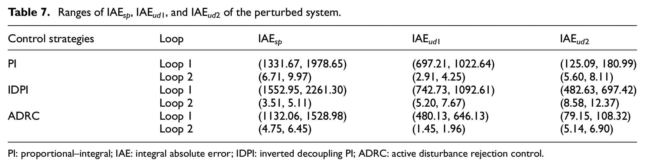
PI: proportional–integral; IAE: integral absolute error; IDPI: inverted decoupling PI; ADRC: active disturbance rejection control.

According to Table 7, ADRC indicates its advantages in robustness. Following are some remarks.

In terms of Loop 1, ADRC has the narrowest ranges of IAE_sp, IAE_ud1, and IAE_ud2. In addition, all indices of ADRC have smallest upper-lower limits

As for Loop 2, the IAE_ud1 and IAE_ud2 of ADRC are perturbed within narrowest ranges. However, IAE_sp of IDPI has the smallest upper-lower limit and narrowest perturbed range, which illustrates the advantage of IDPI in tracking of Loop 2.

Generally speaking, superiorities of ADRC in the power control and exhaust temperature control of the GT have been validated by simulations with respect to reference tracking, disturbance rejection, and robustness.

Variable working condition operation

In the daily operation of a power plant generated by the GT, the unit operates in the wide load range of 50%–100% and the load command is regulated frequently. However, as mentioned in section “Control difficulties analysis,” the nonlinearity of the system is strong. As a result, the dynamic characteristics of power and exhaust temperature change significantly during the variable working condition operation of the GT.

In this subsection, suppose that the load command is changing during the simulation. The set points of the power and the exhaust temperature are changing with the load command. The variation of the load command is illustrated in Figure 15.

Figure 15.

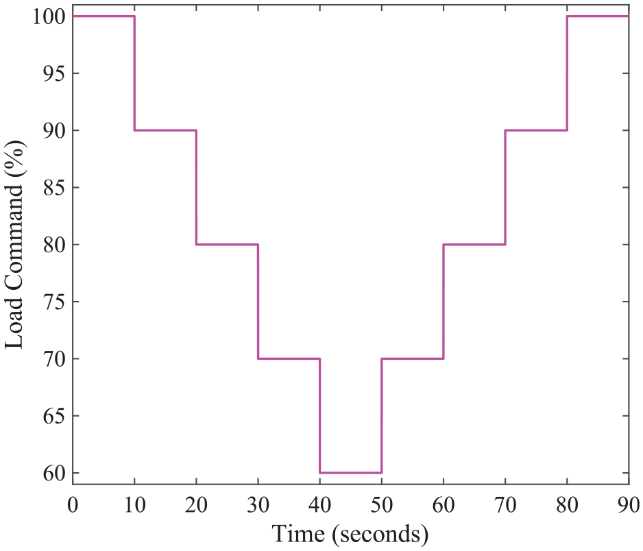
The variation of load command.

According to Figure 15, the load command varies between 100% load and 60% load. It is decreasing in first 40 s and start to increase at 50 s.

Figures 16 and 17 illustrate the variations of power and exhaust temperature when the GT is under the variable working condition operation. In addition, Figure 18 shows variations of manipulated variables.

Figure 16.

Variations of power under variable working condition operation.

Figure 17.

Variations of exhaust temperature under variable working condition operation.

Figure 18.

Variations of manipulated variables under variable working condition operation.

From Figure 16, in terms of power control, it is obvious that ADRC has the smallest overshoot or undershoot at all working conditions. Moreover, the output of ADRC is able to track the set point fastest.

According to Figure 17, as for the control of exhaust temperature, IDPI illustrates its advantages in tracking around the nominal working condition. However, it is unable to track the set point accurately at off-design operating points when the GT is under the variable working condition operating. On the contrary, ADRC is able to track the set point precisely at all working conditions. Besides, it has smaller overshoot or undershoot and faster tracking speed than PI.

Eventually, some remarks are summarized as follows:

The output power of ADRC is able to track the set point effectively when the GT is under the variable working condition operation.

As for the control of exhaust temperature, IDPI is unable to track the set point at off-design operating points for the reason that inverted decouplers are designed based on the nominal transfer functions. However, note that the transfer function is the approximation of the nonlinear mechanism model which may be inexplicit.

Compared with PI, ADRC has better control performance of exhaust temperature when the working condition is changing frequently.

Conclusion

The GT is a typical internal combustion engine with coupling between different control loops and the dynamic characteristic which changes significantly with the working condition. In this article, the decentralized ADRC is designed for the control of power and exhaust temperature of the GT in order to solve these problems. The control difficulties such as strong nonlinearity and coupling are analyzed based on the gap measurement and the frequency-dependent RGA, respectively. Then the design of ADRC is derived theoretically which illustrates ADRC has the ability to estimate and compensate uncertainties of the process. Based on the decentralized structure, numerical simulations are carried out to illustrate that ADRC is able to obtain satisfactory tracking performance and disturbance rejection performance at the nominal operating point. Moreover, the advantage of ADRC in robustness is validated by Monte Carlo trials. Finally, the GT is under the variable working condition operation to test the control performance of ADRC at off-design operating points. Simulation results show that using ADRC is able to enhance the control performance of power and exhaust temperature when the working condition is changing frequently. This successful application indicates the promising prospect in future field tests of multivariable control of the GT based on ADRC. The future work will focus on the field implementation of the decentralized ADRC to the GT.

Footnotes

Declaration of conflicting interests

The author(s) declared no potential conflicts of interest with respect to the research, authorship, and/or publication of this article.

Funding

The author(s) disclosed receipt of the following financial support for the research, authorship, and/or publication of this article: This study was funded by the National Science and Technology Major Project of China 2017-V-0005-0055. The authors also received financial support from the State Key Lab of Power systems, Tsinghua University.

ORCID iD

Gengjin Shi

References

Ghorbani

Ghaffari

Rahnama

Constrained model predictive control implementation for a heavy-duty gas turbine power plant. WSEAS Trans Syst Cont 2008; 3: 507–516.

Najimi

Ramezani

MH.

Robust control of speed and temperature in a power plant gas turbine. ISA Trans 2012; 51: 304–308.

Design and optimization on speed controller of gas turbine. Master’s thesis, Northeastern University, Shenyang, China, 2016.

Han

From PID to active disturbance rejection control. IEEE Trans Ind Electron 2009; 56: 900–906.

Shi

, et al. Research on cascade active disturbance rejection control of superheated steam temperature based on gain scheduling. In: Proceedings of the 19th international conference on control, automation and systems, Jeju, Korea, 15−18 October 2019, pp. 1426–1431. New York: IEEE.

Gao

Scaling and bandwidth-parameterization based controller tuning. In: Proceedings of the American control conference, Denver, CO, 4–6 June 2003, pp. 4989–4996. New York: IEEE.

, et al. Superheated steam temperature control based on modified active disturbance rejection control. Control Eng Pract 2018; 83: 83–97.

Shi

Guo

, et al. Superheated steam temperature based on a hybrid active disturbance rejection control. Energies 2020; 13: 1757.

Zheng

Dong

Lee

, et al. Active disturbance rejection control for MEMS gyroscopes. IEEE Trans Control Syst Technol 2009; 17: 1432–1438.

10.

Huang

Xue

Active disturbance rejection control for the ALSTOM gasifier benchmark problem. Control Eng Pract 2013; 21: 556–564.

11.

Fang

Yuan

Liu

Active-disturbance rejection-control and fractional-order-proportional-integral-derivative hybrid control for hydroturbine speed governor system. Meas Control 2018; 51: 192–201.

12.

Shi

, et al. Maximum sensitivity-constrained data-driven active disturbance rejection control with application to airflow control in power plant. Energies 2019; 12: 231.

13.

Xue

Zhang

Sun

, et al. Extended state filter based disturbance and uncertainty mitigation for nonlinear uncertain systems with application to fuel cell temperature control. IEEE Trans Ind Electron. Epub ahead of print 1 January 2020. DOI: 10.1109/TIE.2019.2962426.

14.

Sun

Yang

, et al. Sample-data-based event-triggered active disturbance rejection control for disturbed systems in networked environment. IEEE T Cybern 2019; 49: 556–566.

15.

Wang

, et al. Application of LADRC with stability region for a hydrotreating back-flushing process. Control Eng Pract 2018; 79: 185–194.

16.

Zhang

Feng

Zhou

, et al. Linear active disturbance rejection control of waste heat recovery systems with organic Rankine cycles. Energies 2012; 5: 5111–5125.

17.

Yuan

Fei

, et al. Hybrid model-based feedforward and fractional-order feedback control design for the benchmark refrigeration system. Ind Eng Chem Res 2019; 58: 17889.

18.

Xue

, et al. Gain scheduling design based on active disturbance rejection control for thermal power plant under full operating conditions. Energy 2019; 185: 744–762.

19.

Sun

Hua

Shen

, et al. Multi-objective optimization for advanced superheater steam temperature control in a 300MW power plant. Appl Energy 2017; 208: 592–606.

20.

Guo

Zhao

On the convergence of an extended state observer for nonlinear systems with uncertainty. Syst Control Lett 2011; 60: 420–430.

21.

Active disturbance rejection control design and application in thermal energy system. PhD thesis, Tsinghua University, Beijing, China, 2019.

22.

Skogestad

Simple analytic rules for model reduction and PID controller tuning. J Process Control 2003; 13: 291–309.

23.

Zhang

Xue

, et al. On the flexible operation of supercritical circulating fluidized bed: burning carbon based decentralized active disturbance rejection control. Energies 2019; 12: 1132.

Decentralized active disturbance rejection control design for the gas turbine

Abstract

Keywords

Introduction

The model of the GT

Mechanism model

Transfer function model

Control difficulties analysis

Design of the control systems

Structures of the multivariable control system

ADRC

Comparative control strategies

Simulation results

Reference tracking

Disturbance rejection

Robustness test

Variable working condition operation

Conclusion

Footnotes

Declaration of conflicting interests

Funding

ORCID iD

References