Dynamic flexible job shop scheduling method based on improved gene expression programming

Abstract

Dynamic scheduling is one of the most important key technologies in production and flexible job shop is widespread. Therefore, this paper considers a dynamic flexible job shop scheduling problem considering setup time and random job arrival. To solve this problem, a dynamic scheduling framework based on the improved gene expression programming algorithm is proposed to construct scheduling rules. In this framework, the variable neighborhood search using four efficient neighborhood structures is combined with gene expression programming algorithm. And, an adaptive method adjusting recombination rate and transposition rate in the evolutionary progress is proposed. The test results on 24 groups of instances with different scales show that the improved gene expression programming performs better than the standard gene expression programming, genetic programming, and scheduling rules.

Introduction

Production manufacturing process is vital to a manufacturing company’s survival and growth, where scheduling plays a key role in determining the overall efficiency and productivity. Scheduling has attracted lots of research attention, but much of traditional research focused on static scheduling, where system state is known in advance and not subject to change throughout the scheduling process. However, actual production environment often encounters dynamic and unexpected events. For example, new jobs may arrive randomly, job processing times may vary, and machines may break down during the production process. All these dynamic events negatively affect the manufacturing process, often rendering the static scheduling solution infeasible and thus resulting in reduced production efficiency and sapped revenue. Therefore, it is more realistic to consider dynamic events in the scheduling, and dynamic flexible job shop scheduling problem (DFJSP) emerges as a promising problem, which has received increasing research attention in the past years.^1,2

Since the work of Jackson ³ that introduced the dynamic scheduling problem in the 1950s for the first time, the dynamic scheduling problem has gained enormous popularity in the scheduling research community, and fruitful results have been reported in the literature, which can be classified into three main categories, namely, rescheduling,^4–10 robust scheduling,^11–14 and online scheduling.^15–18

Rescheduling is also known as pre-reaction scheduling, which implies to schedule again when new events occur. It consists of two stages, the first stage, the pre-scheduling stage, aims to generate a scheduling plan to be followed by actual production; and the second stage, also named as the rescheduling stage, adjusts some or all the original scheduling plans to accommodate the dynamic events happening at a certain moment during production. Usually, some algorithms are used for rescheduling and need some computation time. The rescheduling methods maybe not suitable for some real-time scheduling problems.

Robust scheduling takes into account the system robustness during the scheduling process, strives to anticipate possible future events based on the current manufacturing condition, and generates a pre-schedule that encompasses various dynamic events, which is to ensure that the performance of the scheduling system will not deteriorate when dynamic events occur. However, since the dynamic events will happen uncertainly, the robust scheduling may make the scheduling plan less effective if the dynamic events do not happen.

Online scheduling is also known as real-time scheduling, fully reactive scheduling, and so on. Unlike the above-mentioned two scheduling types, it is a real-time scheduling strategy that does not generate a schedule in advance and is usually used after dynamic events occur, where a certain strategy is used to make a decision for scheduling. In an environment where dynamic events occur frequently, online scheduling can improve system stability and is therefore widely used in actual production.

Aside from limited research on multi-agent technology, ¹⁴ online scheduling research mainly focuses on designing scheduling rules, also named as heuristic rules or dispatching rules. They are used to select jobs for machines or assign machines to jobs. There exist some well-recognized scheduling rules in the literature, including SPT (shortest processing time) rules, EDD (earliest due date) rules, and FCFS (first come first served) rules. It is observed that a particular rule may perform superior to other rules regarding a specific criterion. However, dynamic scheduling problems often involve multiple criteria, a rule suitable for a certain criterion can hardly dominate other criteria. To address this problem, a hybridization of multiple scheduling rules is more appealing to produce better scheduling results. Initial attempts have been made to produce hybrid rules manually, which is often time-consuming and not adaptive. In recent years, promising strides have been made to generate hybrid rules using artificial intelligence algorithms such as genetic programming, ¹⁹ gene expression programming (GEP),^20,21 and other data mining algorithms.

GEP^22,23 was proposed by Ferreira in 2001. It is a machine learning algorithm that combines the advantages of genetic algorithm (GA) and genetic programming (GP). GEP has been widely used in function discovery, rule construction, and prediction. Zhou et al. ²⁴ proposed a new algorithm based on simulated annealing and GEP, and used it to solve the traveling salesman problem (TSP). Guo et al. ²⁵ adopted the principle of gene silencing from biology to tackle the symbolic regression problem, and proposed an improved GEP based on the gene silencing mechanism. Zhang and Liu ²⁶ combined the tabu search with GEP for the prediction of relations between leaching rate of rare earth mineral and the density of its mother liquid. In terms of workshop schedule, Nie et al.^20,21 applied the basic GEP for dynamic job shop scheduling problems and DFJSPs with job release date. Liao ²⁷ combined GEP with biogeography-based optimization, proposed a hybrid biogeography-based gene expression programming algorithm, and constructed a corresponding framework for scheduling rule discovery.

Therefore, the GEP provides a viable approach for solving scheduling problems through extracting useful empirical knowledge and constructing effective scheduling rules. To the best of the authors’ knowledge, Nie et al. ²¹ is the only attempt in the literature to use GEP for flexible job shop dynamic scheduling problems. However, the traditional GEP suffers from disadvantages such as inferior local search capability and poor population diversity. This paper intends to overcome the disadvantages and proposes an improved GEP algorithm for the DFJSP.

In the following sections, the description and mathematical formulation of DFJSP are first introduced. Then, the improved GEP for flexible job shop scheduling problem (FJSP) is presented in detail, followed by the description of the variable neighborhood search algorithm that is used to improve the local search capability of GEP, and the transposition operators used for promoting population diversity. We also explain the framework proposed for solving dynamic scheduling problems based on the improved GEP. Testing instances are then presented and computational results are given. The final section summarizes our work.

DFJSP

Problem description

In a typical dynamic flexible job shop, there are m available machines and n jobs to be processed. The arrival times for these n jobs to the workshop are uncertain. Each operation of a job can be processed on multiple machines. It is necessary to determine the processing machine for each operation and the processing sequence of the operations on each machine so as to obtain the optimal scheduling solution. In a production workshop, before each operation of a job is processed, some preparation work will be done on the corresponding machine, such as adjustment and clamping. This period is usually called the setup time. ²⁸ In the traditional scheduling problem research, the setup time is usually ignored or used as a part of the processing time. However, in the actual processing, the switch between different processes will lead to different setup times, so the makespan of the job will be affected as well. Therefore, it is necessary to separate the setup time from the processing time in the DFJSP.

Some basic assumptions are listed as follows:

1. No order constraints exist among jobs;

2. A job can only be processed on one machine at a time;

3. A machine can only process one job at a time;

4. Machine preemption and interruption are not allowed;

5. The processing order among the operations of a job is fixed;

6. An operation can be assigned to multiple candidate machines for processing;

7. Machines are available at the initial moment, regardless of machine failure.

Mathematical model

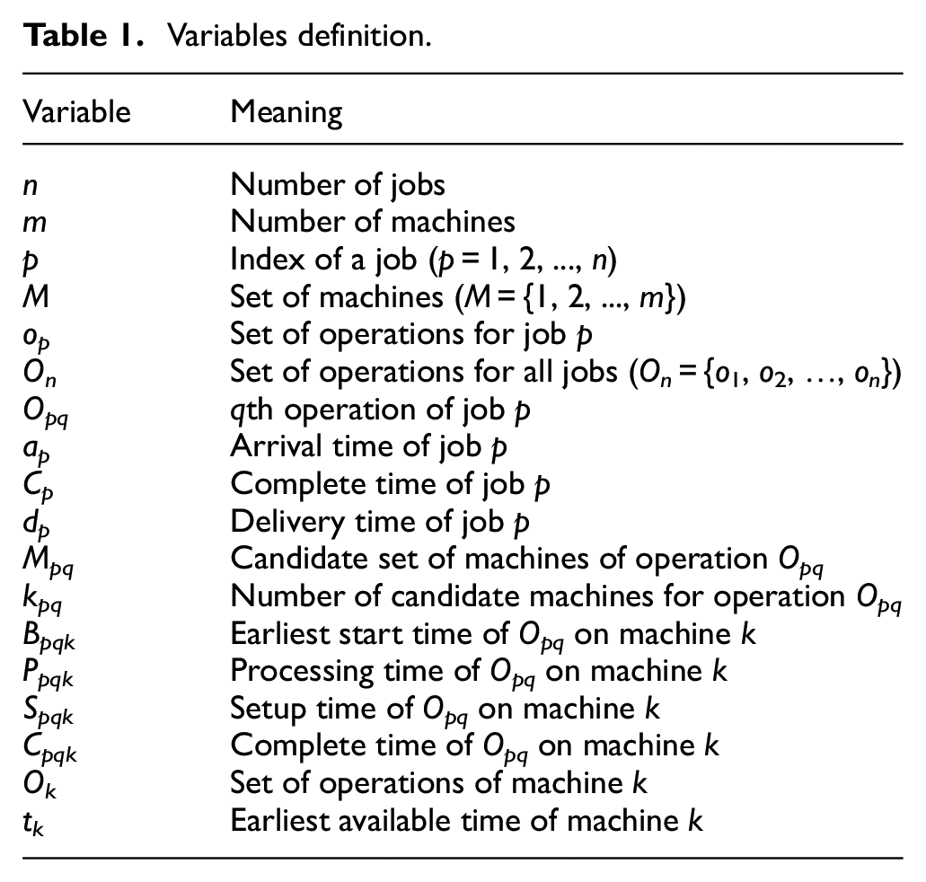
The mathematical model of the DFJSP considering separate setup time is given. The variables used in the model are listed in Table 1.

Table 1.

Variables definition.

Variable	Meaning
n	Number of jobs
m	Number of machines
p	Index of a job (p = 1, 2, …, n)
M	Set of machines (M = {1, 2, …, m})
op	Set of operations for job p
On	Set of operations for all jobs (On = {o1, o2, …, on})
Opq	qth operation of job p
ap	Arrival time of job p
Cp	Complete time of job p
dp	Delivery time of job p
Mpq	Candidate set of machines of operation Opq
kpq	Number of candidate machines for operation Opq
Bpqk	Earliest start time of Opq on machine k
Ppqk	Processing time of Opq on machine k
Spqk	Setup time of Opq on machine k
Cpqk	Complete time of Opq on machine k
Ok	Set of operations of machine k
tk	Earliest available time of machine k

All constraints are presented as follows

$$P_{\mathrm{pqk}}>0p=1,2,\dots ,n$$

(1)

$$C_{\mathrm{pq}{k}^{\prime }}\ge C_{p(q-1)k}+P_{\mathrm{pqk}\prime }p=1,2,\dots ,n$$

(2)

$$\sum _{k=1}^m{X}_{\mathrm{pqk}}=1p=1,2,\dots ,n,q=1,2,\dots ,o_p$$

(3)

$$\sum _{p=1}^n{X}_{\mathrm{pqk}}\le 1q=1,2,\dots ,o_p,k=1,2,\dots ,m$$

(4)

$$\begin{array}{c}\multicolumn{1}{c}{B_{p1k}=\max (a_p,t_k)+S_{p1k}p=1,2,\dots ,n,}\\ \multicolumn{1}{c}{k=1,2,\dots ,m}\end{array}$$

(5)

$$\begin{array}{c}\multicolumn{1}{c}{B_{\mathrm{pqk}}=\max (C_{p(q-1)k\prime },(t_k+S_{\mathrm{pqk}}))q=2,\dots ,o_p,}\\ \multicolumn{1}{c}{k,k\prime =1,2,\dots ,m}\end{array}$$

(6)

$$B_{\mathrm{pqk}}\ge C_{p\prime q\prime k}+S_{\mathrm{pqk}}$$

(7)

$$C_{\mathrm{pqk}}=B_{\mathrm{pqk}}+P_{\mathrm{pqk}}p=1,2,\dots ,n,q=1,2,\dots ,o_p$$

(8)

$$C_p=\max C_{\mathrm{pqk}}q=1,2,\dots ,n_p$$

(9)

X_pqk is the decision variable

$$X_{\mathrm{pqk}}=\{\begin{array}{cc}1\hfill & \mathrm{if}{O}_{\mathrm{pq}}\mathrm{is}\mathrm{processed}\mathrm{by}\mathrm{machine}k\hfill \\ \multicolumn{1}{c}{0}& \mathrm{otherwise}\hfill \end{array}$$

(10)

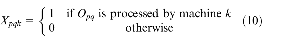
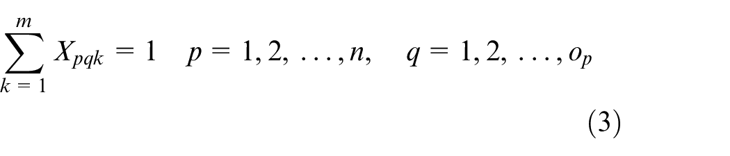
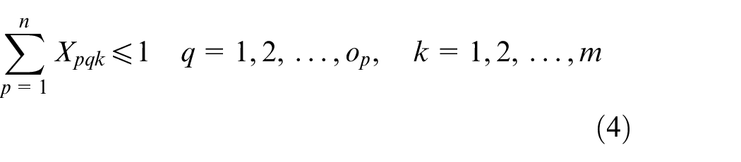
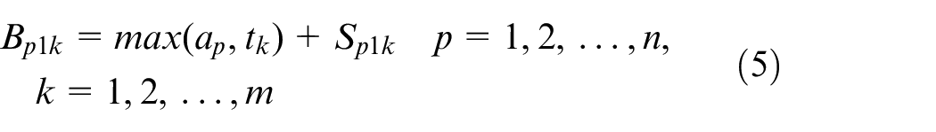
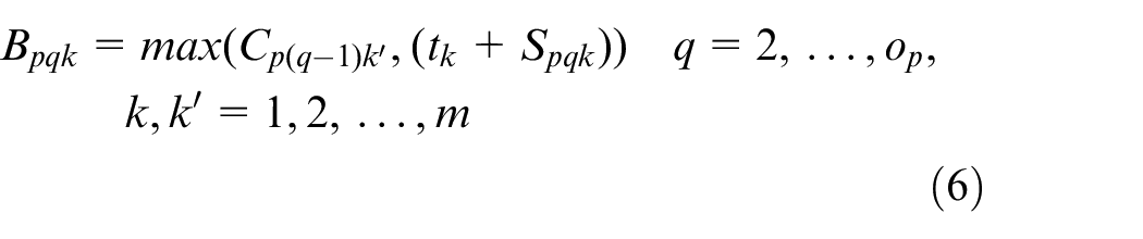
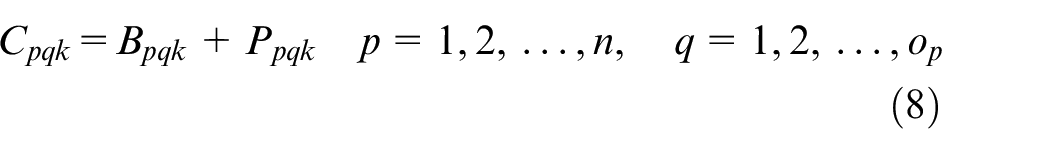
Constraint (1) ensures that the processing time for each operation is positive. Constraint (2) shows the complete time constraint between two adjacent operations. The constraint that a job can only be processed on one machine at a time is given in equation (3), and the constraint that a machine can only process one job at a time is presented in equation (4). The start time of the first operation for each job is calculated by equation (5). Since the arrival time cannot be known in advance, the start time of the first operation can be known after the job arrivals. The start time for other operations except the first operation is obtained by equation (6). Constraint (7) indicates that the operation on a machine cannot start only after the last operation on the machine and the setup is finished. The complete time for each operation is calculated by equation (8), and the complete time for a job is the complete time of its last operation, which is shown in equation (9). The objective function is to minimize the makespan t_ms shown in equation (11)

$$t_{\mathrm{ms}}=\max \left\{C_P|p=1,2,\dots ,n\right\}$$

(11)

Improved GEP for DFJSP

The original GEP

Basic steps

GEP is a variant from combining GA and GP, and its basic steps are similar to GA:

• Step 1. Set the parameters and initialize the population.

• Step 2. Calculate the fitness value for individuals in the population and check the termination condition. If the termination condition is satisfied, output the best solution found. Otherwise, go to step 3.

• Step 3. Select individuals by the roulette wheel selection.

• Step 4. Perform genetic operators for the selected individuals.

• Step 5. Generate a new population, and go to step 2.

Encoding and decoding

In the GEP, a gene is composed of a fixed-length string, which can be divided into two parts, the head and the tail, which are important components of the whole gene. The relationship between the tail length t and the head length h is shown in equation (12), where s is the number of all parameters in the predefined function set (FS) in GEP. The element in the head of the gene can be selected from FS and terminal set (TS), while the element in the tail can only be selected from TS. Chromosomes in GEP may be composed of more than one gene

$$t=h*(s-1)+1$$

(12)

The encoding of GEP adopts the “head + tail” way. After the expression tree is obtained, the depth-first traversal method can be used to traverse the expression tree to obtain the final desired expression. Conversely, using a depth-first approach can also decode strings into expression trees.

Genetic operators

Genetic operators include selection, recombination, transposition, and mutation. These operators are introduced briefly as follows:

1. Selection: the roulette wheel selection with elitism is adopted in the original GEP.

2. Recombination: GEP usually uses one-point recombination, two-point recombination, and gene recombination.

3. Transposition: transpositions are unique operators in GEP. There are three kinds of transpositions including IS (insertion sequence elements) transposition, RIS (root IS elements) transposition, and gene transposition. IS transposition means that a gene fragment is first randomly selected and then inserted into other elements except for the first element at the head of the gene. At the same time, the gene segment with the same length as the insert is deleted at the end of the head, keeping the head and tail of the entire gene to ensure the whole length unchanged. The difference between root insertion sequence elements transposition and IS transposition is that the selected inserted gene segment can only start with an element of the head, and the insertion position is only at the top of the gene head. Gene transposition is only used in multi-gene chromosomes. Firstly, a gene is randomly selected and then moved to the head of the entire chromosome and the original gene is deleted.

4. Mutation: GEP used one-point mutation which is the same as GA.

Improved GEP

GEP inherits the strong global search ability from GA, but its local search ability is limited. The variable neighborhood search ²⁹ (VNS) searches by constructing different neighborhood structures and constantly searches for new and better local optimal solutions by changing the neighborhood structure near the current local optimal solution. Because of its strong local search ability, VNS has been used to solve various combinatorial optimization problems. Embedding the VNS in GEP can greatly improve the local search capability of GEP. At the same time, in order to overcome the shortcomings of poor population diversity in the late evolution, an adaptive genetic operator is used to guide the search process of the algorithm, and part of the population is updated after evolving over a certain number of generations.

VNS

According to the characteristics of the shop scheduling problem, four neighborhood structures are constructed in the VNS:

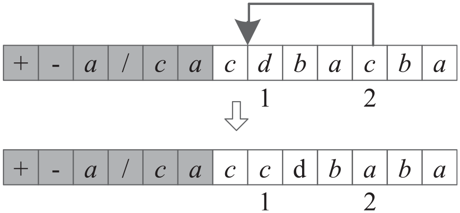
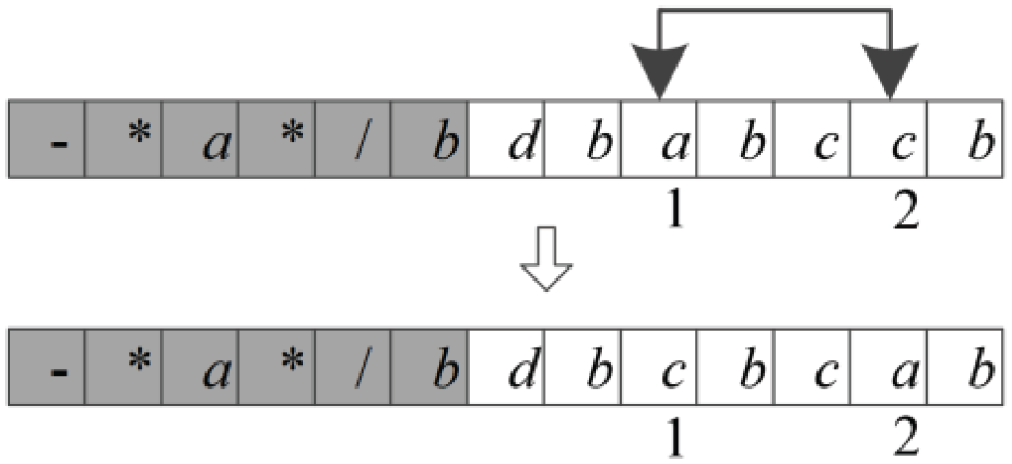
1. Insert neighborhood: randomly select two elements from the tail of the gene and insert the element in the latter position before the one in the previous position, as shown in Figure 1.

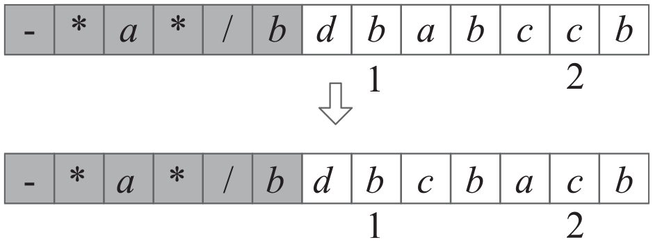
2. Swap neighborhood: two elements are randomly selected in the tail of the gene, and the elements at the two positions are swapped with each other, as shown in Figure 2.

3. Rearrangement neighborhood: randomly select four elements from the tail of the chromosome, and shuffle their positions as shown in Figure 3.

4. Inverse neighborhood: randomly select two positions in the tail of the chromosome, then arrange the elements between the two positions in reverse order, as shown in Figure 4.

Figure 1.

Insert neighborhood.

Figure 2.

Swap neighborhood.

Figure 3.

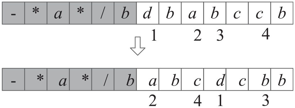
Random rearrangement neighborhood.

Figure 4.

Inverse neighborhood.

In the GEP, the population evolves by the guidance of the genetic operators, and then, some individuals are selected for executing the VNS; the steps are described as follows:

1. Rank all the individuals in the population according to their corresponding fitness values in decreasing order.

2. Select the individuals ranking on the top as the elite solutions, denoted as population M.

3. Half of the solutions selected randomly from M, and the other half selected randomly from the other solutions are executed VNS.

Adaptive genetic operator rate

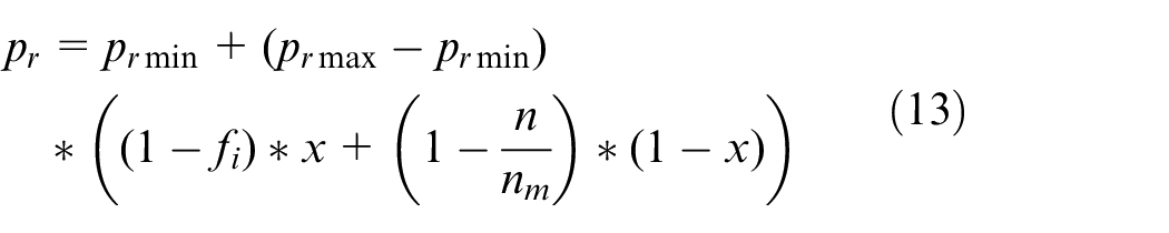
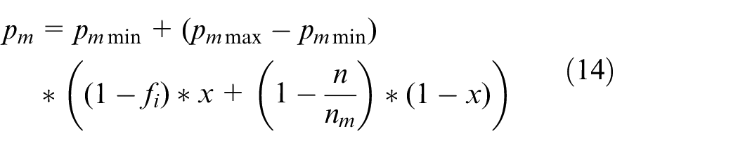
Parameters such as recombination rate and transposition rate play important roles in GEP. However, using fixed parameters throughout the whole evolutionary process is not conducive to the convergence of the algorithm. An adaptive genetic operator is proposed to autonomously adjust the parameters during the evolutionary process. The new recombination rate and transposition rate in GEP are shown in equations (13) and (14), respectively.

In equation (13), p_r is the recombination rate, p_rmin is the minimum recombination rate, p_rmax is the maximum recombination rate, f_i is the fitness value of individual i, x is a weighting factor between 0 and 1, n is the number of successive iterations that the population is not improved, and n_m is the maximum number of successive iterations that the population is not improved. This formula shows that as the iteration progresses, the fitness value of the individual and the current number of unimproved iterations both affect the recombination rate.

In equation (14), p_m is the transposition rate, p_mmin is the minimum transposition rate, p_mmax is the maximum transposition rate, and the others are the same as in equation (13).

In the early stages of population evolution, poor individuals are given a higher recombination rate and transposition rate, which may accelerate the evolution of the individuals. The individuals with better fitness values are given a lower recombination rate and transposition rate, so as to protect the good individuals. In the late stage of population evolution, there is still a certain probability for poor individuals to update to prevent the algorithm from the premature convergence. This adaptive setting method for the two genetic rates can balance the convergence and the diversity of the population

$$\begin{array}{c}\multicolumn{1}{c}{p_r=p_{rmin}+(p_{rmax}-p_{rmin})}\\ \multicolumn{1}{c}{*((1-f_i)*x+(1-\frac{n}{n_m})*(1-x))}\end{array}$$

(13)

$$\begin{array}{c}\multicolumn{1}{c}{p_m=p_{mmin}+(p_{mmax}-p_{mmin})}\\ \multicolumn{1}{c}{*((1-f_i)*x+(1-\frac{n}{n_m})*(1-x))}\end{array}$$

(14)

Improved GEP for shop dynamic scheduling

Fitness value

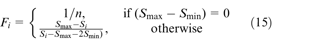
When using GEP to solve the dynamic scheduling problem, the fitness function is shown in equation (15), where F_i represents the fitness value of the ith chromosome, n is the population size, S_i represents the objective function value corresponding to the scheduling rule represented by the ith chromosome, S_max represents the maximum value of the objective function, and S_min represents the minimum value of the objective function

$$F_i=\{\begin{array}{cc}1/n,\hfill & \mathrm{if}(S_{\max }-S_{\min })=0\hfill \\ \multicolumn{1}{c}{\frac{S_{\max }-S_i}{S_i-S_{\max }-2S_{\min })},}& \mathrm{otherwise}\hfill \end{array}$$

(15)

FS and TS

Scheduling rules can be composed of a combination of parameters of jobs, machines, and so on in the workshop scheduling. Therefore, some parameters of jobs and machines are used as the element source of the TS, and the relationship between these parameters can be used to construct the FS:

1. FS.

   The elements of the FS for the improved GEP include “+, -, *, /.” When the divisor is 0, 1 will be obtained by the element “/.”

2. TS.

   The constructed elements of the TS are shown in Table 2, where JTS (job terminal set) and MTS (machine terminal set) represent the TS for job allocation and machine selection, respectively.

Table 2.

Elements in the terminal set.

(JTS) relevantto job	Meaning	(MTS) relevantto machine	Meaning
JRD	Arrival time of a job	OPT	Operation timeof the current operationprocessed by a machine
ORT	Arrival time of the currentoperation of a job	OST	Setup time of the current operation on a machine
OBT	Earliest start time of thecurrent operation of a job	MRON	Number of operations unfinished on a machine
OPT	Processing time of the currentoperation processed by a machine	MROT	Total processing time for the unfinished operationson a machine
OST	Setup time of the currentoperation on a machine	MFON	Number of finished operations on a machine
SL	Slack time for a job	MFOT	Total processing time for the finished operationson a machine
JUON	Number of operationsunfinished for a job	MT	Earliest available time for the current machine
UOPT	Sum of average processing timeof operations unfinished for a job
OT	Idle time for a job
WT	Waiting time of machines for a job
JDD	Due date for a job

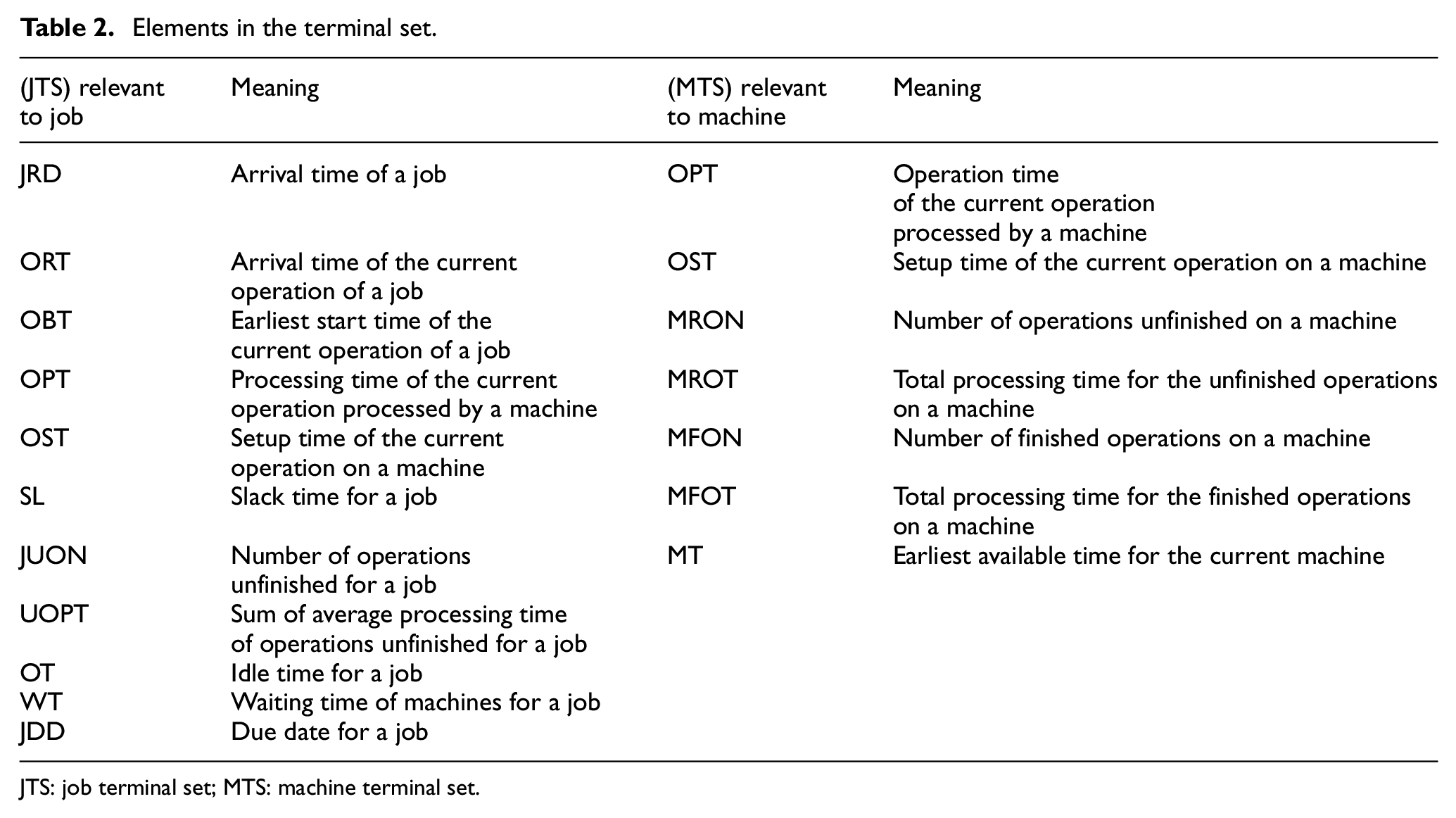
JTS: job terminal set; MTS: machine terminal set.

The average processing time $\overline{P_{\mathrm{pq}}}$ for each operation is shown in equation (16), where k_pq represents the number of candidate machines for operation O_pq, and P_pqk is the processing time of O_pq by machine k

$$\overline{P_{\mathrm{pq}}}=\frac{\sum _{k=1}^{k_{\mathrm{pq}}}{P}_{\mathrm{pqk}}}{k_{\mathrm{pq}}}$$

(16)

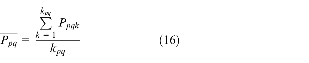
In Table 2, the arrival time of the current operation is the finish time of its last operation. The earliest start time of the current operation is shown in equation (17), where MT is the earliest available time of the assigned machine. The slack time SL is shown in equation (18), where CT is the current time. The idle time of a job is presented in equation (19), and the waiting time of a machine is shown in equation (20)

$$\mathrm{OBT}=\max (\mathrm{ORT},\mathrm{MT})$$

(17)

$$\mathrm{SL}=(\mathrm{JDD}-\mathrm{CT}-\mathrm{UOPT})$$

(18)

$$\mathrm{OT}=max(0,\mathrm{CT}-\mathrm{ORT})$$

(19)

$$\mathrm{WT}=max(0,\mathrm{ORT}-\mathrm{CT})$$

(20)

Since terminal elements include JTS and MTS, there are two parts about job and machine in the chromosome. The elements for operation assignment come from JTS and FS. The elements for machine selection are from MTS and FS. Figure 5 shows a multiple-gene chromosome constructed by the above encoding method, where one gene is used for job assignment and the other one for machine selection. The head parts are shown in shadow and other parts are the tail parts. The decoding method takes a depth-first approach.

Figure 5.

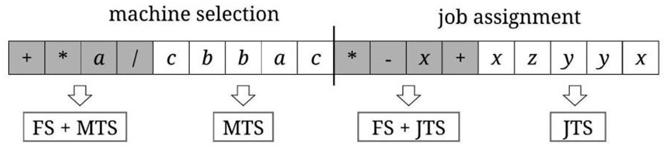
Multi-gene chromosome.

Framework and steps

A dynamic shop scheduling framework based on the improved GEP is proposed, as shown in Figure 6. In the framework, the evaluation module is the core module. Since there is no pre-determined data set and no evaluation criteria for dynamic scheduling, a simulation evaluation system is constructed based on the parameters related to jobs and machines in the shop and applied to evaluate the constructed scheduling rules. In the rule construction module, the scheduling rules generated by the population initialization are passed to the evaluation module. The evaluation module evaluates the scheduling rules according to some required performance indicators and performs a series of genetic operations on the population according to the evaluation results to form a new population. The new population is passed into the evaluation module for evaluation. The process is repeated until the termination condition is met. The final output is the scheduling rule.

Figure 6.

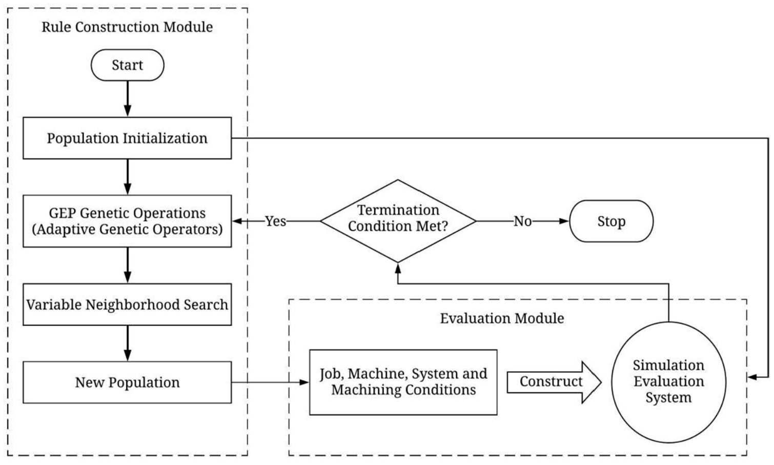
Framework of dynamic shop scheduling based on improved GEP.

The specific steps are as follows:

• Step 1. Algorithm parameters setting, including population size, termination condition, genetic operator rate, number of neighborhoods, and so on.

• Step 2. Random initialization of the population, according to the constructed FS and TS, initialize the machine selection and job allocation parts, respectively.

• Step 3. Calculate the fitness value of the individuals and check whether the termination condition is met. If it is met, the algorithm stops and outputs the result, otherwise, go to step 4;

• Step 4. Use the roulette wheel with elite reservation to perform the selection operation. The selected individuals are reorganized and shifted according to the adaptive recombination rate and transposition rate. At the same time, each individual in the population is mutated according to the given mutation rate.

• Step 5. Sort the fitness value of the population after the above operations, select individuals for VNS, and perform VNS for them.

• Step 6. Check whether the number of iterations where the optimal solution has not updated does reach the preset value. If so, randomly generate some individuals to replace the worst individuals in the current population. Otherwise, go to step 7.

• Step 7. Generate a new population through the above operations and evaluate the individuals in the population.

• Step 8. Repeat steps 3–7 until the termination condition is met, and output the result. Here, the termination condition is that the current iteration number reaches to the maximum iteration number.

Experiment and analysis

Experiment setting

A numerical experiment is designed to verify the effectiveness of the proposed algorithm for the DFJSP where the jobs arrive randomly. There are no benchmark problems for the problem, and test cases need to be generated according to the problem characteristics. Table 3 shows the parameter settings for the experiment and improved GEP.

Table 3.

Parameter setting for the experiment and improved GEP.

Problem parameters	Values	Algorithm parameters	Values
Job number	20 (small size), 100 (large size)	Function set	{+, -, *, /}
Machine number	10 (small size), 20 (large size)	Terminal set	As shown in Table 2
Operation number	U[1,10] (small size), U[1,20] (small size)	Joint function	+
		Length of head	11
Processing time	U[1,100]	Length of tail	12
Setup time	U[5,30]	Number of gene	2
Utilization η	75%, 90%	Population size	20
s	1, 2	Mutation rate	0.05
Machine flexibility	20%, 50%, 100%	Recombination rate	[0.1, 0.5]
		Transposition rate	[0.1, 0.4]
		Number of positions in transposition	IS transposition {1, 2, 3}RIS transposition {1, 2, 3}
		Weight factor	0.6

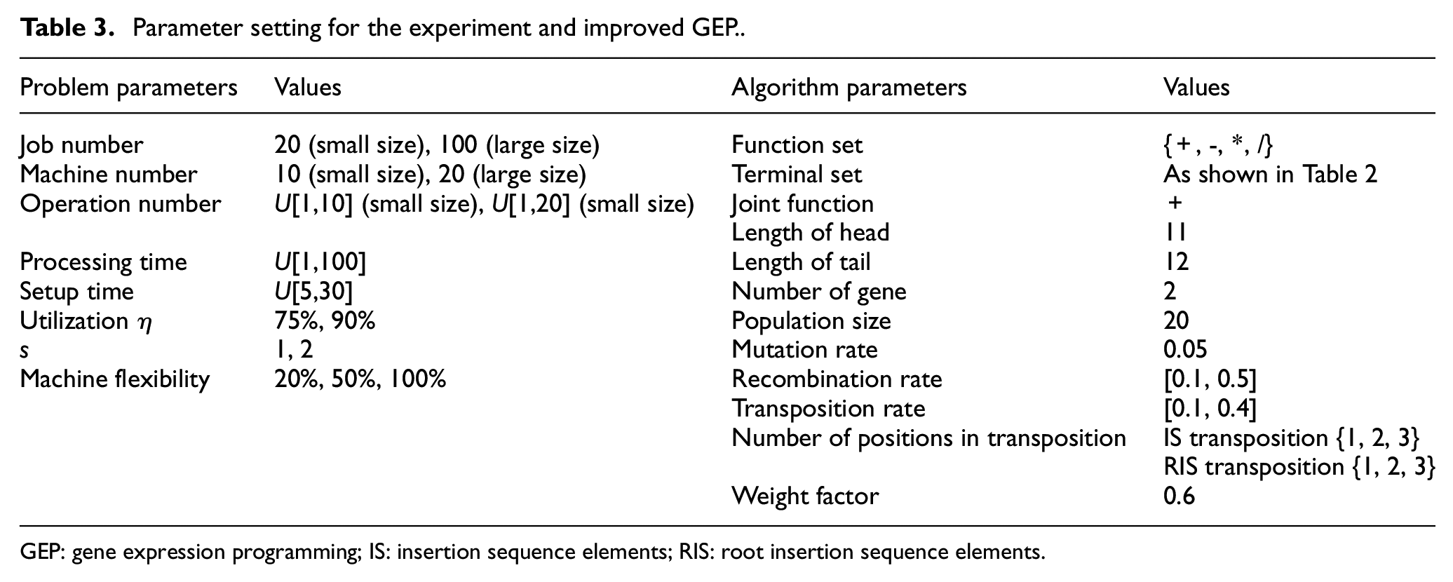
GEP: gene expression programming; IS: insertion sequence elements; RIS: root insertion sequence elements.

Parameter setting for the experiment

Two kinds of test instances with small and large scales are generated in the experiment. The number of jobs is 10 in the instances with a small scale, while 100 for large-scale instances. The number of machines in the two kinds of instances is 10 and 20, respectively. The number of operations for a job obeys uniform discrete distributions within [1,10] and [1,20]. The processing time of each job follows the uniform distribution of [1,100], and the setup time follows the uniform distribution of [5,30]. The parameter s defines the urgency level of a job. The flexibility of the machine indicates the number of machines that can be selected for an operation in the FJSP, and the values are 20%, 50% and 100%, which can be seen in Table 3. Two kinds of scales, three types of machine flexibility, two types of workshop utilization levels, and two types of tension factors together lead to a total of 24 groups of instances, where each group contains 40 random instances and 20 instances are used for training to get dispatch rules and the others for testing.

Assuming the job arrival is a Poisson process, their interval of arrival follows an exponential distribution whose mean interval is shown as (21)

$$\lambda =\frac{\sum _{p=1}^n\sum _{q=1}^{o_p}{P}_{\mathrm{pq}}}{\mathrm{mn}\eta }$$

(21)

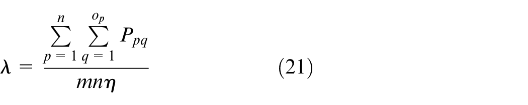
In equation (21), λ is the mean interval, P_pq is the processing time of operation O_pq, o_p is the number of operations for job p, m is the number of machines, n is the number of jobs, and η is the utilization of machines.

Parameter setting for the improved GEP

The parameters in the improved GEP are also listed in Table 3. The parameters for standard GEP and GP are listed in Tables 4 and 5. All programs for the three algorithms are coded by C++. All experiments are run on a personal computer with Intel core i5-3470 (3.20 GHz) and 4 GB RAM, and the operating system is Windows 7.

Table 4.

Parameters for the GEP.

Parameters	Values
Function set	{+, -, *, /}
Terminal set	As shown in Table 2
Length of head	8
Length of tail	9
Gene number	3
Population size	20
Mutation rate	0.05
Recombination rate	One-point recombination: 0.2
	Two-point recombination: 0.2
	Gene recombination: 0.1
Transposition rate	IS transposition: 0.1
	RIS transposition: 0.1
	Gene transposition: 0.1

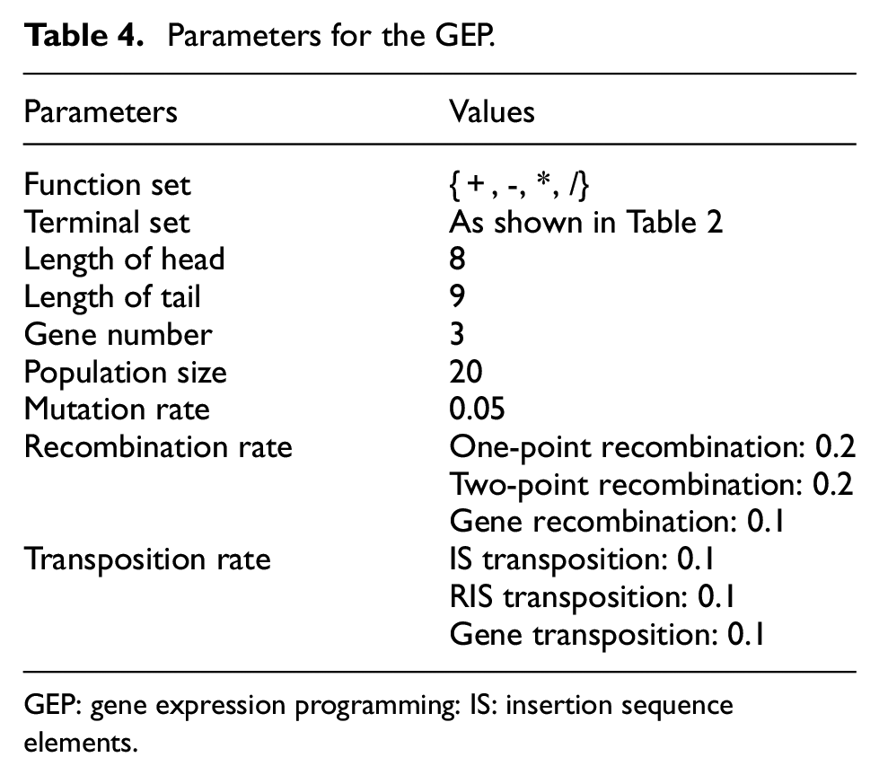
GEP: gene expression programming: IS: insertion sequence elements.

Table 5.

Parameters for the GP.

Parameters	Values
Population size	20
Crossover rate	0.6
Mutation rate	0.3
Maximum depth	6

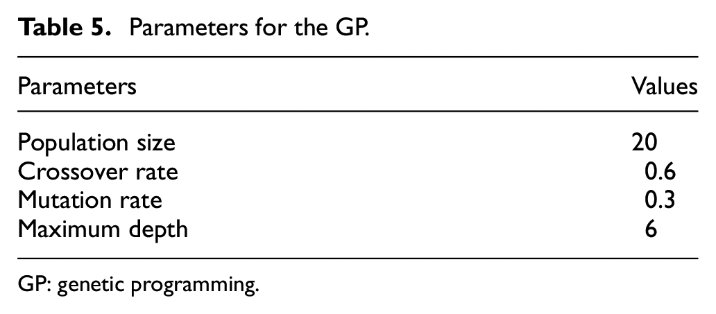
GP: genetic programming.

Since there are two subproblems (machine selection and job assignment) in FJSP, the following methods are used to verify the efficiency of the proposed GEP. The common rule for machine selection is LMT (least waiting time). The rule will select the machine with the least total processing time of the operations waiting for processing. The rules for job assignment generated by the standard GEP and GP and some classic dispatch rules are used for comparison. The above combinations of rules are presented as “LMT/GEP,”“LMT/GP,”“LMT/SPT,”“LMT/EDD,” and “LMT/(SL + SPT).” Some involved dispatch rules are introduced as follows:

• SPT: the rule will select operation with the shortest processing time and it can be represented by OPT.

• EDD (earliest delivery date): the rule will select operation with the earliest delivery date and it can be expressed by JDD.

• SL + SPT: it is a hybrid rule. SL is the slack time of a job, and it can be represented by SL = JDD −  CT − UOPT, where CT is the current time.

The delivery date is calculated as equation (22)

$$d_p=a_p+s\times \sum _{q=1}^{o_p}(\stackrel{-}{P_{\mathrm{pqk}}}+\stackrel{-}{S_{\mathrm{pqk}}})$$

(22)

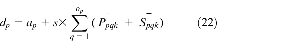
where d_p is the delivery date of job p; a_p is the arrival time of job p; $\stackrel{-}{P_{\mathrm{pqk}}}$ and $\stackrel{-}{S_{\mathrm{pqk}}}$ is the average processing time and setup time on available machines of operation O_pq, respectively; and s is a parameter defining the urgency level of a job.

Each algorithm runs five times, and the average values are used for comparison and the maximum iteration for the improved GEP, GEP, and GP is 1000.

Result analysis

The comparison results for the three algorithms are presented in Table 6, where the values in bold are the best ones among the three algorithms. Take “S1_20_10_10_75%_1_20%” as an example to explain the name of the instance set. “S1” represents the first test set; “20” means the job number is 20; The first value “10” represents the machine number is 10 and the second value “10” means the operation number obeys uniform discrete distributions within [1,10]; “75%” is the machine utilization and the value “1” is the s value in (22); The last value “20%” is the machine flexibility.

Table 6.

Results obtained by different algorithms for solving DFJSP.

Test instances	Improved GEP	LWT/GEP	LWT/GP	LWT/SPT	LWT/EDD	LWT/SL + SPT
S1_20_10_10_75%_1_20%	1319.08	1472.16	1475.09	1543.33	1574.08	1557.72
S2_20_10_10_75%_1_50%	1148.98	1491.56	1487.91	1523.9	1533.53	1515.3
S3_20_10_10_75%_1_100%	1005.69	1451.45	1453.33	1456.6	1467.38	1458.47
S4_20_10_10_75%_2_20%	1283.88	1424.22	1423.03	1508.95	1555.93	1538.68
S5_20_10_10_75%_2_50%	1079.05	1444.26	1442.14	1457.5	1478.85	1481.35
S6_20_10_10_75%_2_100%	1048.28	1474.75	1472.11	1482.82	1488.7	1475.2
S7_20_10_10_90%_1_20%	1204.97	1348.26	1340.08	1449.53	1480.97	1479.4
S8_20_10_10_90%_1_50%	961.72	1343.5	1336.13	1361.03	1375	1379
S9_20_10_10_90%_1_100%	904.45	1354.22	1348.92	1359.33	1377.05	1376.72
S10_20_10_10_90%_2_20%	1152.28	1281.16	1281.43	1361.65	1455.47	1431.2
S11_20_10_10_90%_2_50%	975.06	1333.25	1336.93	1372.63	1373.6	1373.7
S12_20_10_10_90%_2_100%	829.35	1276.38	1279.57	1289.32	1298.4	1330
S13_100_20_20_75%_1_20%	4327.88	4955.28	4957.21	5127.13	5138.95	5124.5
S14_100_20_20_75%_1_50%	4014.38	4868.86	4870.56	4893.8	4906.48	4897.52
S15_100_20_20_75%_1_100%	4083.86	4985.9	4981.28	5001.55	5002.25	5002.2
S16_100_20_20_75%_2_20%	4299.9	4937.43	4924.18	5008.7	5074.77	5061.35
S17_100_20_20_75%_2_50%	4174.3	4989.15	5010.18	5042	5072.15	5067.1
S18_100_20_20_75%_2_100%	4093.92	4991.05	4994.37	5042	5072.15	5067.1
S19_100_20_20_90%_1_20%	3694.21	4364.78	4371.68	4573.13	4647.5	4671.77
S20_100_20_20_90%_1_50%	3508.02	4443.43	4425.88	4496.95	4593.35	4566.68
S21_100_20_20_90%_1_100%	3420.63	4339.95	4343.28	4375	4398.02	4386.45
S22_100_20_20_90%_2_20%	3683.85	4356.57	4362.05	4526.07	4627.93	4629.85
S23_100_20_20_90%_2_50%	3499.78	4387.2	4399.63	4475	4559.8	4541.45
S24_100_20_20_90%_2_100%	3401.73	4359.75	4353.42	4391.8	4433.08	4433.95

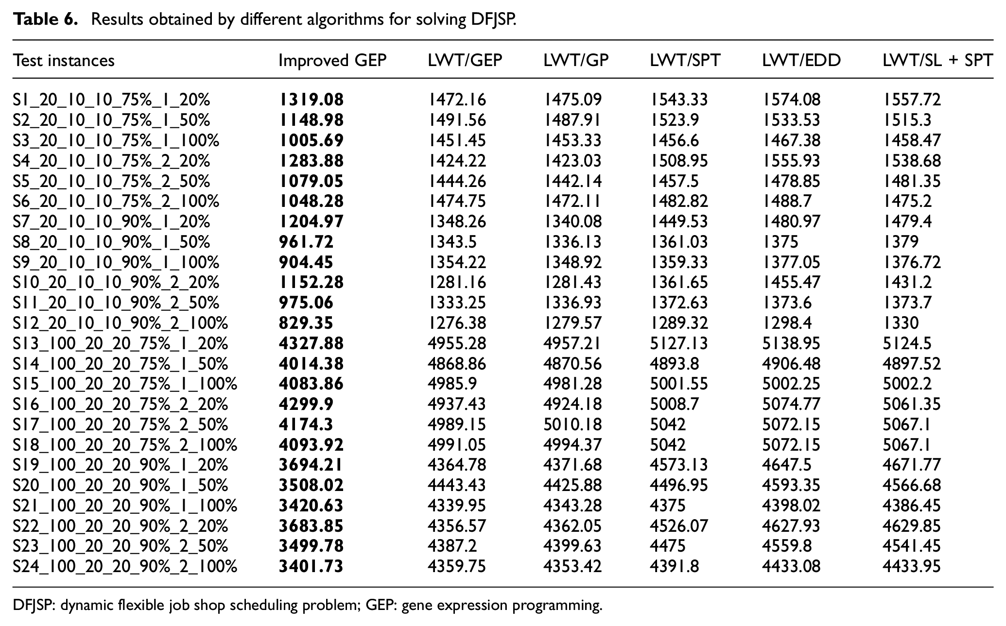
DFJSP: dynamic flexible job shop scheduling problem; GEP: gene expression programming.

Taking the instances S2_20_10_10_75%_1_50% and S3_20_10_10_75%_1_100% as an example, the scheduling rules obtained by the improved GEP, which can get the best makespan among the five runs, are shown in equations (22) and (23), respectively. The upper part in each formula is the rule for machine selection and the lower part is the rule for job assignment. The meaning of the variables is shown in Table 2. For the rules of machine selection, when the objective function is the makespan t_ms, the processing time OPT on the machine is an important parameter except for the MROT which is the only parameter MROT in LWT. Compared with the corresponding instance for equation (24), the instance for equation (23) has lower machine flexibility and the suitable machine for a job is harder to be found, so the rule for machine selection in equation (23) is more complex than the rule in equation (24). The rule includes the parameters MROT, MFON, OST, and so on, except OPT. For the machine where the total processing time for the unfinished operations is less, the number of finished operations and the setup time of the current operation is less, having higher priority in the machine selection

$$\begin{array}{c}(\mathrm{OPT}+\mathrm{MROT})*\mathrm{OPT}+\mathrm{MFON}+\mathrm{OST}\hfill \\ (\frac{\mathrm{OT}}{\mathrm{OBT}}-\mathrm{JUON})*(\mathrm{JOUN}-\mathrm{OPT})\hfill \end{array}$$

(23)

$$\begin{array}{c}\mathrm{OPT}\hfill \\ (\mathrm{WT}-\frac{\mathrm{UOPT}}{\mathrm{JUON}})*\mathrm{JRD}\hfill \end{array}$$

(24)

It can be observed from Table 6 that the average makespan under the rules obtained by the improved GEP is much better than that under the classical scheduling rules and the rules obtained by the other two algorithms both on small-scale and large-scale problems. The makespan under the rules obtained by the improved GEP is smallest on all the instances and the efficiency of the improved GEP is verified. Meanwhile, when the rule for machine selection is LWT, the rule for job assignment obtained based on GEP and GP can get smaller makespan for most instances than the other classical scheduling rules. The classical scheduling rule SPT is better than EDD and the compound rule “SL + SPT.” The rule EDD and the compound rule “SL + SPT” show similar performance, which indicates that a compound rule is not always better than a single rule.

Conclusion and future work

An improved GEP-based dynamic scheduling method was proposed for solving the DFJSP considering setup time and random job arrival. The variable neighborhood search is embedded into the GEP, and multiple neighborhood structures are designed for improving the local search ability. Meanwhile, a method for adaptively setting the genetic operator rate is introduced to alleviate the premature convergence problem. Some worse individuals are replaced in the latter search process to improve the diversity of the population. A framework based on the improved GEP is proposed. Twenty-four groups of test instances are generated, and the improved GEP is compared with standard GEP, GP, and other classical scheduling rules. The comparison results demonstrate the efficiency of the improved GEP.

The most critical point when using GEP to construct scheduling rules is the selection of FS and TS elements. At the same time, the constructed scheduling rules are sometimes complicated and difficult to understand. How to design the TS to ensure that the resulting scheduling rules are efficient and easy to understand is a major focus of future research. This work only focuses on the random arrival of jobs. In the future, dynamic events such as machine failures, insertion orders, and change of delivery time can also be considered. At the same time, other objectives such as energy efficiency^30,31 can also be considered in the future.