
Abstract
Data envelopment analysis is a nonparametric method for measuring of the performance of decision-making units—which do not need to have or compute a firm’s production function, which is often difficult to calculate. For any manager, the progress or setback of the thing they manage is important because it makes planning and adoption of future policies for the organization or decision-making unit more rational and scientific. Different methods have been used to calculate the improvements and regressions using Malmquist Index. In this article, we evaluate the units under review in terms of economic efficiency, and the units in terms of spending, production, revenue and profit over several periods, and the rate of improvement or regression of each of these units. Considering the minimal use of resources and consuming less money, generating more revenue, and maximizing profits, the improvement or retreat of the recipient’s decision unit in terms of cost, revenue, and profit was examined by presenting a method based on solving linear programming models using the productivity index is Malmquist and Malmquist Global. Finally, by designing and solving a numerical example, we emphasize and test the applicability of the material presented in this article.
Keywords
Introduction
The concept of cost efficiency is that measuring the ability of a decision-making unit (DMU) to produce outputs at the lowest input cost, which Farrell began in 1957. He defined cost efficiency as the minimum cost to actual cost. 1 Since 1978, Charnes et al. 2 have started data envelopment analysis which we are using now and have become widely used by researchers to examine firms’ performance with inputs, outputs, and technology. One of the important aspects of using DMUs is the measurement of cost and revenue efficiency. 3
In 1978, Farrell introduced the data envelopment analysis (DEA) method by implementing Charnes, Cooper, and Rhodes (CCR) model as a performance measurement method. This way it incorporates multi-input and multi-output production process features and provides unit-scale output when measuring efficiency. In 1982, Luss 4 introduced the classic problem of capacity development, and its aim is to minimize the cost of the whole process. Lee and Johnson 5 proposed in 2014 a short-term capacity planning approach.
Nicola Alder and Nicola Volta 6 in 2016 used the economically oriented distance function to examine external and consumer outcomes. Ahangari and Rostamy-Malkhalifeh 7 investigated earnings inefficiency with interval data. Sahoo et al. 8 used the directional distance function for economic efficiency. Kazutoshi et al. 9 measured the minimum inefficiency gap in DEA. Rostamy and his colleagues started working on inefficiency in 2019. In 2015, He et al. 10 examined the stability and sensitivity radius for uncertain boundaries. Inuiguchi and Mizoshita 11 studied quality and quantity in interval data in 2012. Jahanshahloo et al. 12 studied on interval data. Allahyar and Rostamy-Malkhalifeh13,14 reviewed the performance analysis for negative data and performance-based scalability in 2015 and proposed a method for scaling-up performance 15 and studied supply chain performance in a hybrid way. 16 Very interesting work on economic efficiency was done fuzzily. In 2019, Rahmani and colleagues17–20 conducted activities and research with fuzzy data. In 2018, Roets 21 expressed multiple output efficiency and security. In 2017, Ahmadvand and Pishvaee 22 discussed how to implement the allocation problem based on fuzzy weights.
In 2019, Peykani and Mohammadi 23 proposed a domain-oriented size model of the feasibility of ranking warehouses in the presence of negative and non-linear data. 20 Also, some, like Podinovski et al., 24 used nonparametric production technologies in 2018.
In 2019, Akhlaghi and Rostamy-Malkhalifeh 25 used integer linear programming to determine the most-efficient DMU. 26 Another key issue in DEA is the Malmquist Productivity Index. The Malmquist Index was first introduced in 1953 as a qualitative index in the analysis of consumer inputs by Stan Malmquist and became well-known among researchers. In 1982, Caves et al. 27 proposed it for DEA.
Fare et al. (1994) Combined the ideas of Farrell efficiency measurement and also productivity measurement presented by Caves et al. (1982), and decomposed the malmquist productivity index into technical efficiency changes and (frontier) technology changes. It should be noted that, the malmquist productivity index represents the productivity changes over time. Malmquist Index has some drawbacks despite being widely used, including when dealing with linear programming techniques. For the calculation of the index, the invariance occurs which is a fundamental problem in the data structure. And, sufficient data were obtained to resolve the problem, 28 and Pastor and Lovell29,30 showed that the source of the problem is the properties of adjacent step technologies in the index building.
Berg et al. (1992) 31 generalized the definition of the Malmquist index in the context of cross-section-time-series data by introducing a base or reference technology. Portela and Thanassoulis (2008) proposed a Meta-Malmquist index under the Constant Returns to Scale (CRS) and Variable Returns to Scale (VRS) technologies. This index can be decomposed into the circular components of efficiency and technical change.
However, each of the Malmquist Indicators does not solve all three problems. Then, a new index is built from all data at all stages and periods of all manufacturers, and its technology was presented as the Global Malmquist that has a circular feature. It measures the magnitude of productivity change. The Malmquist Global Index can solve all three problems by specifying a fixed boundary. In 2012, Tohidi et al. 32 used the Malmquist Global in cost estimation. Emrouznejad and Yang 33 used Malmquist Global to investigate carbon dioxide emissions. Tohidi and Razavyan used Malmquist Global in 2012 to calculate the profit of DMUs. Not all articles present and research on the economic productivity (cost, income, and profit) of economic units were reviewed. For more details, refer to Khodabakhshi et al. (2010), Nikfarjm et al. (2015), Zadeh (1965), Wang and Jiang (2012) and Toloo et al. (2008).
In this article, we examine the economic development of new entities in terms of cost consumption and income generation and profitability. This article is composed of the following sections. Section “Basic model of performance in DEA” presents the basic model of calculating efficiency and defining efficiency. Section “Economic efficiency (cost, income, and profit efficiency)” deals with the definition of economic efficiency. Sections “Malmquist Global” and “Calculating economic productivity improvement and regression with the Malmquist Global Index” present calculation of the economic productivity improvements and regressions using section “Malmquist Global”; the numerical example with the models and methods presented is presented in the final section of the dissolution plan.
Basic model of performance in DEA
Data Envelopment Analysis (DEA) is a non-parametric method for evaluating the performance of a group of homogenous decision making units (DMUs) with multiple inputs and multiple Outputs. Charnes et al. (1978) 2 considered the technology with Constant Returns to Scale (CRS) to propose CCR model and then Banker et al. (1984) 34 considered the technology with Variable Returns to Scale (VRS) to propose BCC model.
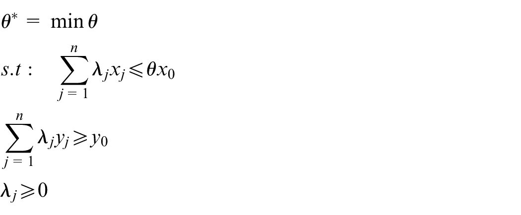
If n is the decision unit (DMUj, j = 1, 2, 3, …, n) that uses m to produce the output S and the vectors xj = (x1j, …, xmj) and yj = (y1j, …, ysj) are the inputs and outputs, respectively. Therefore,
Economic efficiency (cost, income, and profit efficiency)
Consider the problem of minimizing the cost of a company with inputs to produce outputs and cost vector
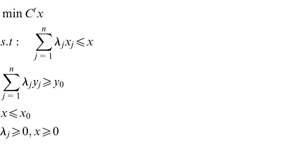
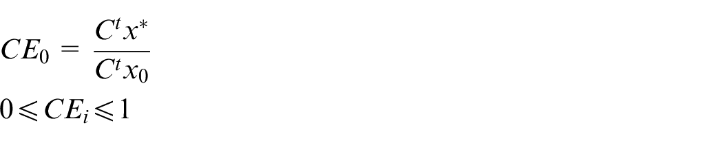
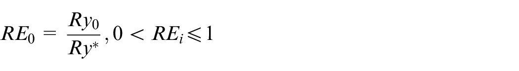
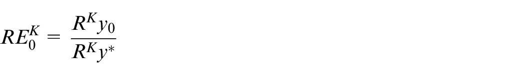
Cost efficiency is the ratio of the minimum cost to the real cost
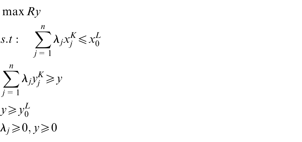
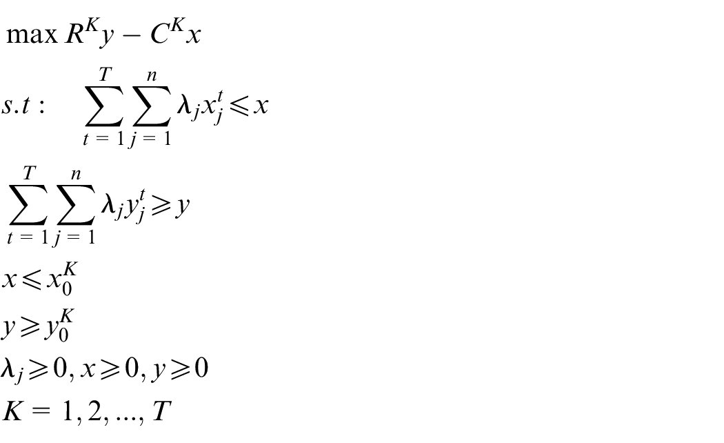
If we want to maximize revenue for units (DMUs), real revenue is provided if the output prices vector r (r≠ 0 and r≥ 0) is specified, and the maximum revenue obtained from the input vector x0 is obtained by solving the following model
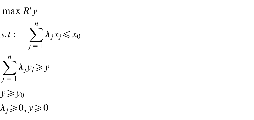
Income efficiency is given as
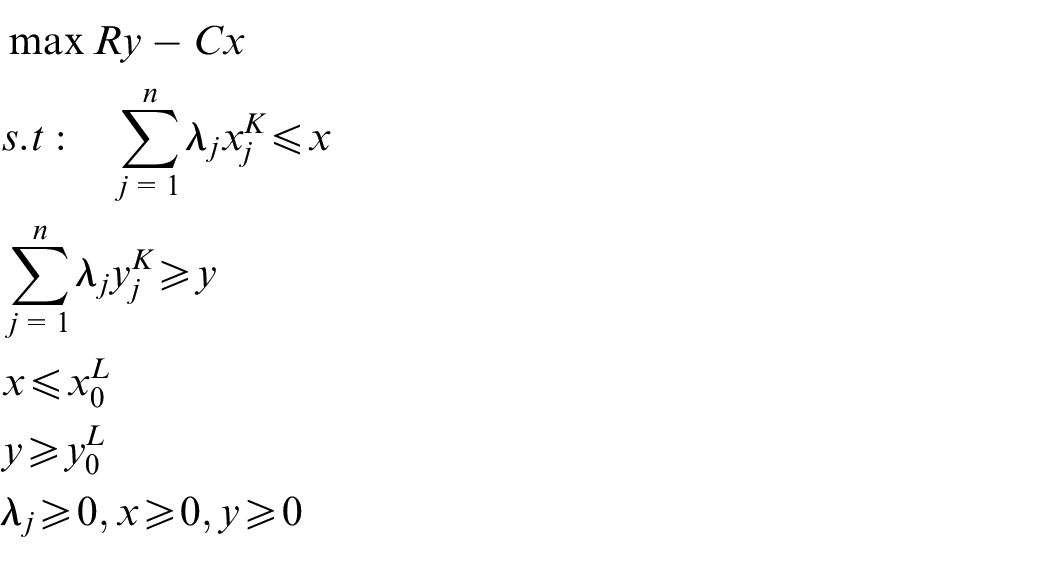
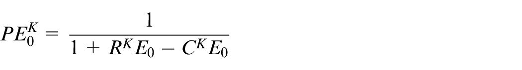
Benefit efficiency is given as
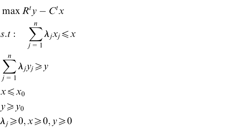
DMU0 is benefit efficiency if
Calculating economic productivity improvement (cost, income, and profit)
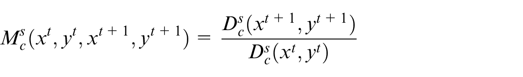
Following the implementation of the CCR economic performance model, we seek to determine whether different decision makers are improved, are regressed, or remain unchanged in terms of their performance over different time periods. Accordingly, using the Malmquist Index, the performance improvement or regression of the units is analyzed. Malmquist Index measurement requires calculation of distance functions.
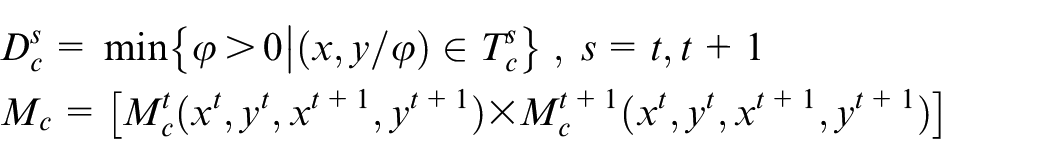
To solve these functions, we can use the linear programming method of comprehensive data analysis. In this regard, for each DMU, according to the Malmquist Index between two time periods t and t+1, four distance functions must be calculated, which in turn requires solving four linear programming problems. Assuming constant-scale returns (assumed by Färe et al. in their analysis 28 ), four issues will be addressed and solved for cost efficiency
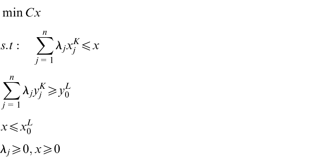
(unit in time L—border in time K); K = t, t+ 1, L = t, t+ 1.
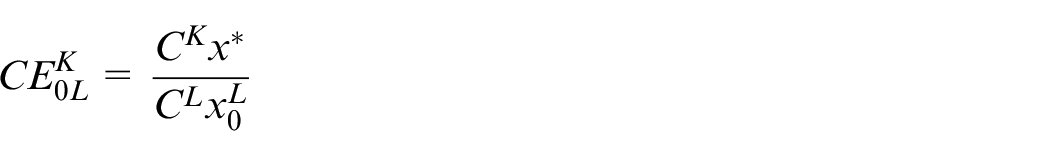
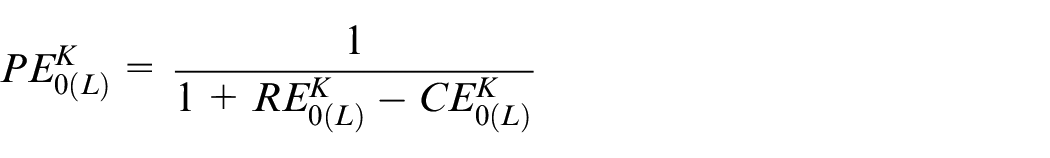
Cost effectiveness is given as
We can calculate the Malmquist Index for the cost efficiency of DMU0 using the following equation

where CMPI0 > 1 indicates the improvement in cost efficiency of DMU0 from time period t to time period t+ 1, CMPI0 = 1 indicates the recovery of DMU0 cost efficiency from time period t to time period t+ 1, and CMPI0 < 1 indicates the unchanged cost efficiency of DMU0 from time period t to time period t+ 1
(unit in time L—border in time K); K = t, t+ 1, L = t, t+ 1.
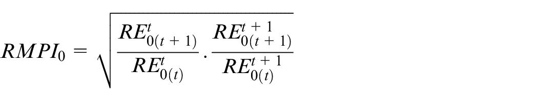
Income efficiency is given as
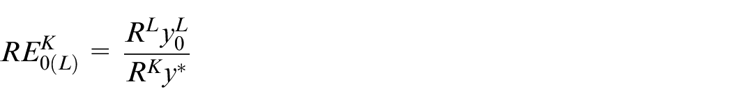
Using the following equation, we can calculate the Malmquist index for DMU0’s earnings efficiency
where
where L = t, t+ 1 is the unit in time and K = t, t+ 1 is border in time, and also, we can get the benefit efficiency using the equation below
The Malmquist Index for DMU0 profitability is derived from the following relation
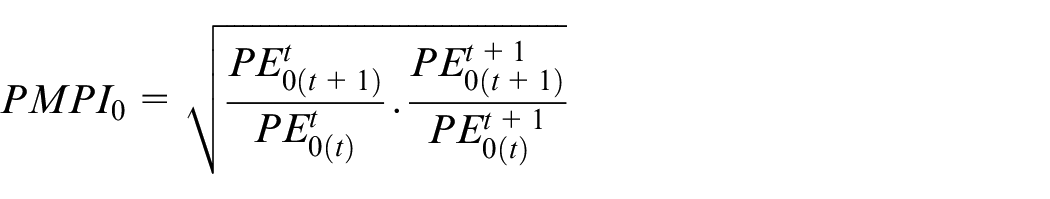
where PMPI0 > 1 shows the improvements, PMPI0 < 1 shows the regressions, and PMPI0 = 1 shows there is no change.
Malmquist Global
We have DMU0 generating units (0 = 1, 2, …, n) and defined time periods t (t = 1, 2, …, T). Global technology is defined as follows

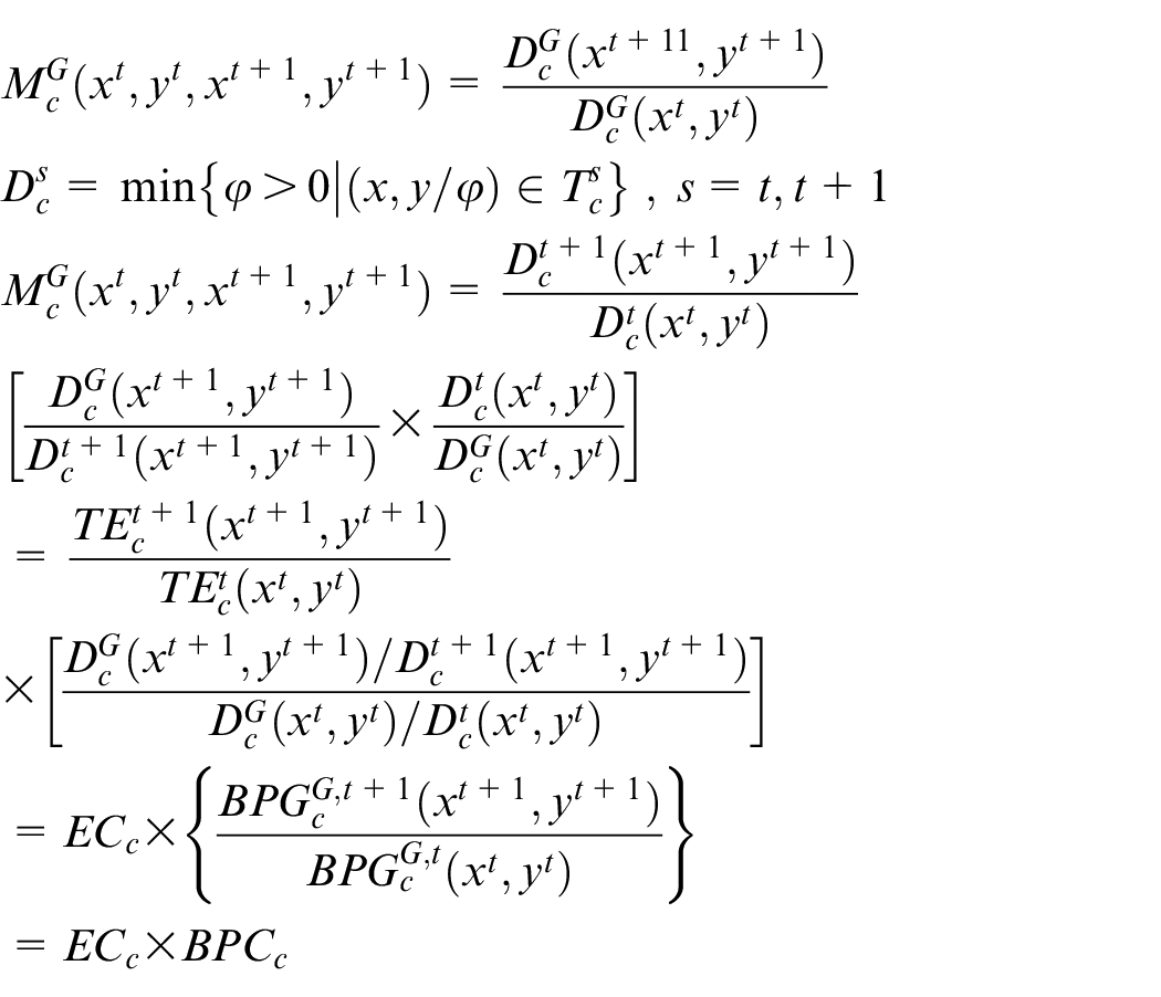
The Malmquist Productivity Index is defined as follows
So
The Malmquist Global Index defined on
Calculating economic productivity improvement and regression with the Malmquist Global Index
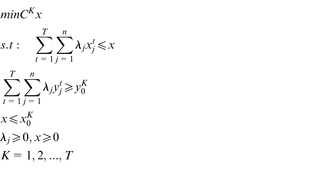
If the units are evaluated over time periods t = 1, 2, 3, …, T, in the Malmquist Global Method, we examine all units in one place, and the cost efficiency model for DMU0 at time k is given below. In this section, each DMU is compared to itself over different time periods, and it has progressed in two periods, such as p and q
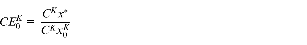
And, the cost efficiency comes from the following relationship
If we consider the productivity of DMU0 at time p compare to time q, we consider the solution of the model K = p, q and two problems raised and are solved. The Malmquist Global Index is written as follows

where if
The income performance model for DMU0 at time K is written as follows. And, each DMU is compared to itself at different times
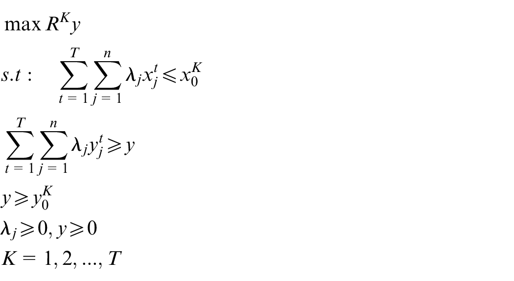
Income efficiency is given as
To evaluate the efficiency of DMU0 at time p compare to time q, we place K = p, q in the model at time p, and two problems are solved. The following is the definition of the Malmquist Global Index

If
We write the profitability model for DMU0 at time K and compare each DMU at different times
Benefit efficiency is given as follows
To evaluate the efficiency of DMU0 at time p compare to time q, we set K = p, q. And, two issues are raised and solved. We define the Malmquist Global Quotient as follows

If
Numerical examples
For example, we consider 10 DMUs with three inputs and two outputs over the three time periods
The inputs and outputs data in three time period for 10 DMUs.
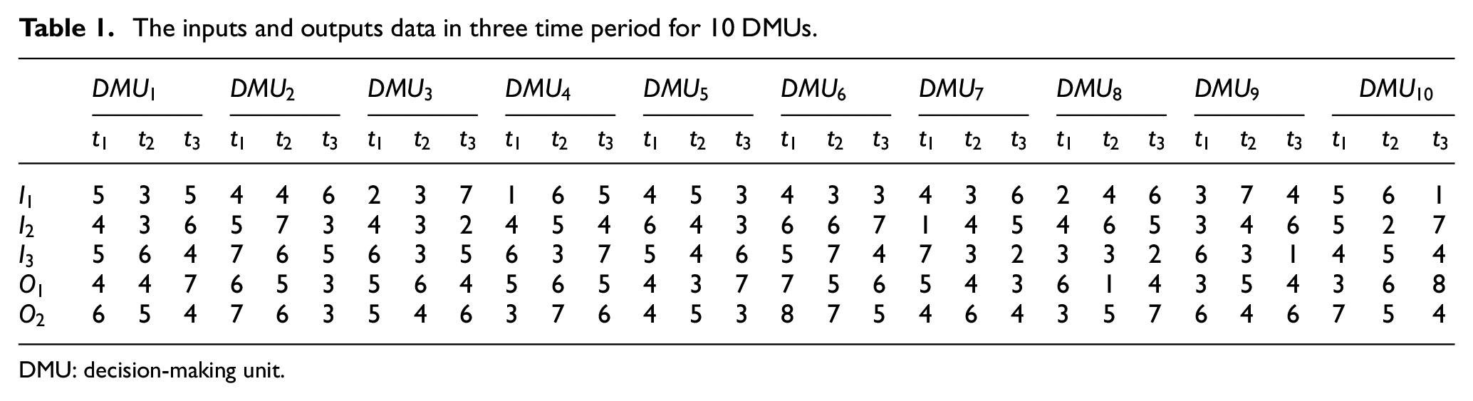
DMU: decision-making unit.
Cost, income, and profit Efficiency in three time period for 10 DMUs.
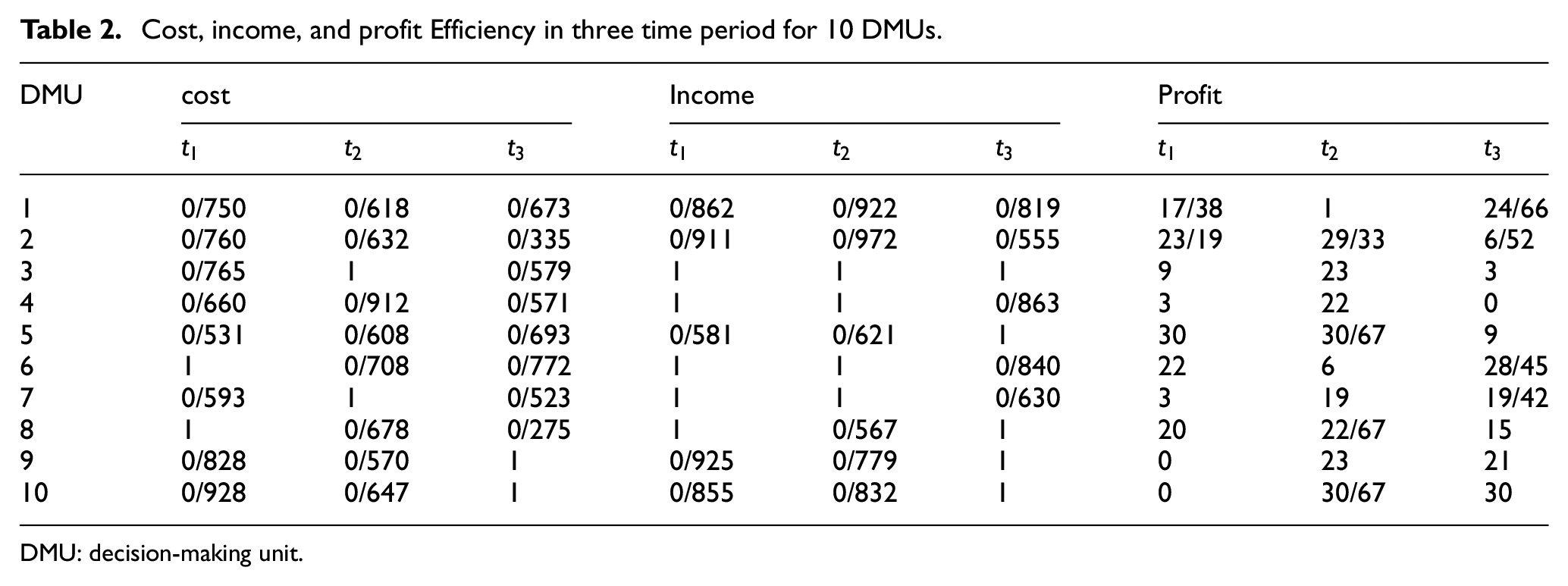
DMU: decision-making unit.
Tables 3–5 show the proposed models for calculating the improvement and regression of units with the Malmquist index from periods t1 to t2, t1 to t3, and t2 to t3.
Economic productivity improvement and regression with the Malmquist Index (t1 to t2).
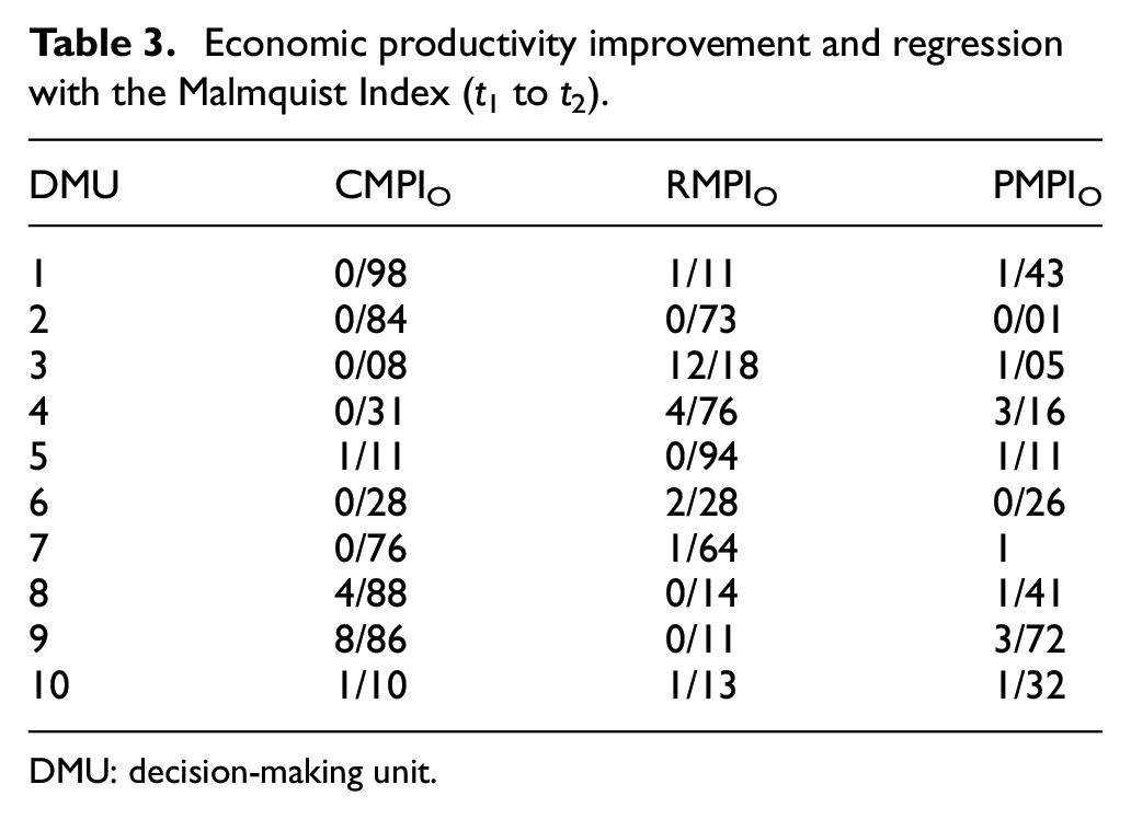
DMU: decision-making unit.
Economic productivity improvement and regression with the Malmquist Index (t1 to t3).
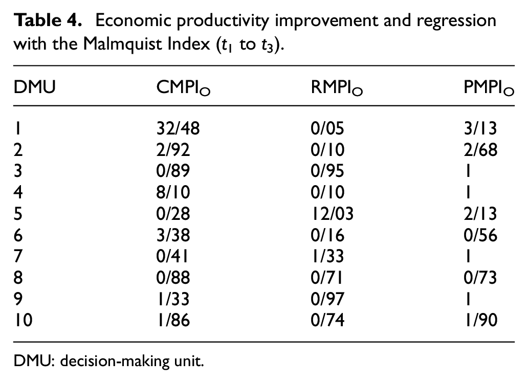
DMU: decision-making unit.
Economic productivity improvement and regression with the Malmquist Index (t2 to t3).
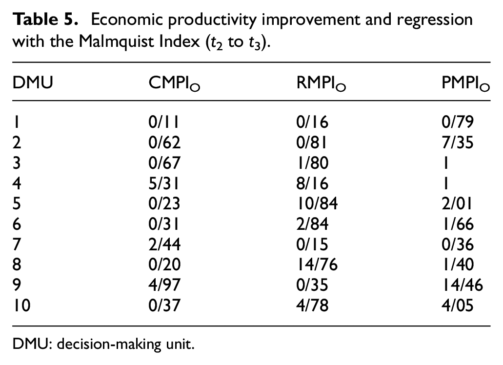
DMU: decision-making unit.
Tables 6–8 show the progression and regression of units with the Malmquist Global Index. We find that the Global Malmquist has the characteristic of being out of the ordinary while the Malmquist lacks, this is the feature. For unit 1, we are avoiding Malmquist Global with respect to cost efficiency index. From the ratio
Cost productivity improvement and regression with the Malmquist Global Index.
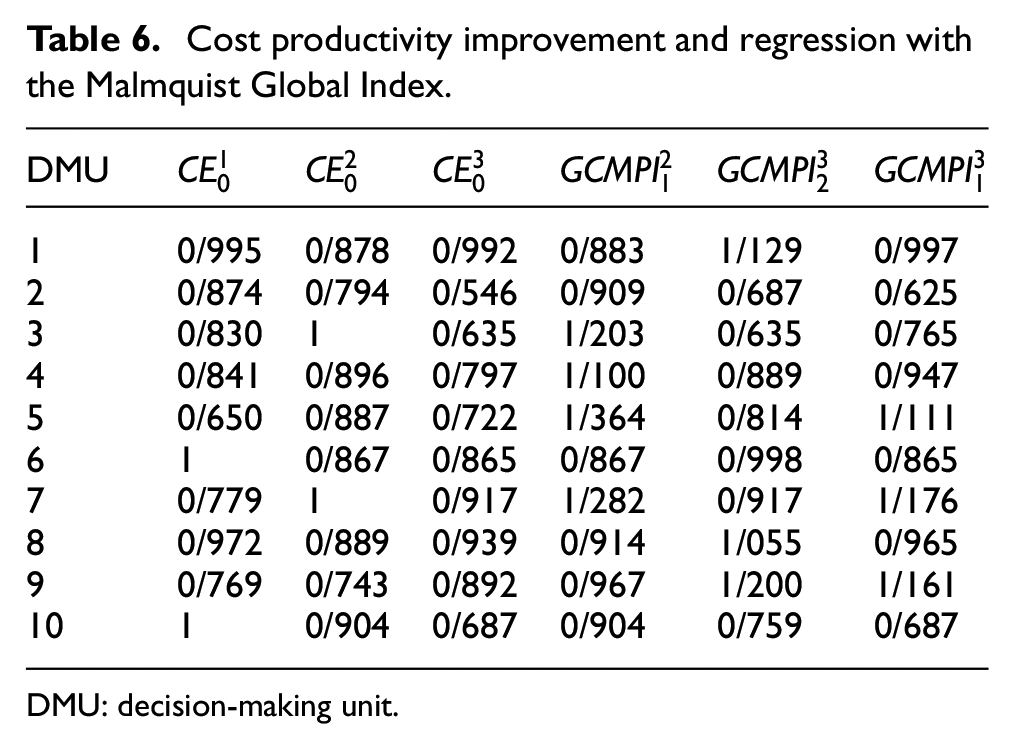
DMU: decision-making unit.
Income productivity improvement and regression with the Malmquist Global Index.
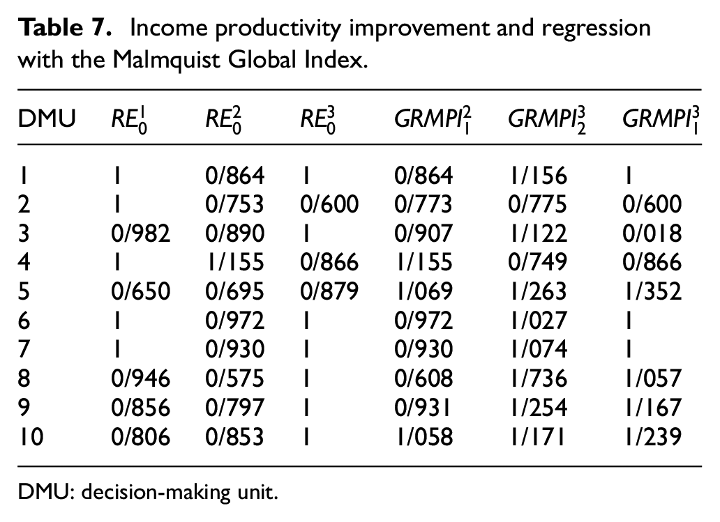
DMU: decision-making unit.
Profit productivity improvement and regression with the Malmquist Global Index.
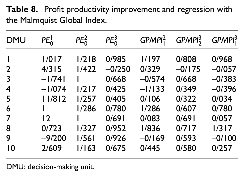
DMU: decision-making unit.
Conclusion
Calculating the Malmquist Productivity Index is a very useful and applicable system for determining the progress and regress of a system and helps managers in future decisions and policies of the system and leads to improved productivity. The Global Malmquist Productivity Index helps managers track the progress and remediation of a system or organization over two time periods, across time periods, and improve decision-making and policy making. And better evaluate the efficiency of a unit.
Footnotes
Declaration of conflicting interests
The author(s) declared no potential conflicts of interest with respect to the research, authorship, and/or publication of this article.
Funding
The author(s) received no financial support for the research, authorship, and/or publication of this article.