Sage Journals: Discover world-class research

Abstract

Vortex flowmeter is a commonly used flow measurement device. It is almost not affected by the density and viscosity of the fluid, so the vortex flowmeter can be used for the detection of various medium, such as gas, liquid and steam. When dealing with vortex street signal, we usually use fast Fourier transform to calculate the signal frequency, but this traditional vortex street signal processing method is not only inefficient, but also difficult to filter out noise signals in the same frequency band as the vortex signal. The sparse Fourier transform utilizes the sparsity of the signal to efficiently calculate the signal spectrum, and the computational complexity is lower than that of the fast Fourier transform algorithm. In this paper, the amplitude and frequency of the vortex signal is analyzed by sparse Fourier transform and the noise signal is removed based on the amplitude–frequency characteristics of the vortex signal. Finally, by comparing with the other methods, we found that the time complexity of our algorithm is one-tenth of others’ methods. This means that our approach is 10 times faster than others.

Keywords

Vortex signal sparse Fourier transform time complexity

Introduction

Vortex flowmeter is a flow detection device based on the famous Karman vortex street principle. As shown in Figure 1, when the fluid passes through a bluff body, it separates and generates alternant vortex. Then, the vortex sensor detects the frequency of the vortex shedding.¹

Figure 1.

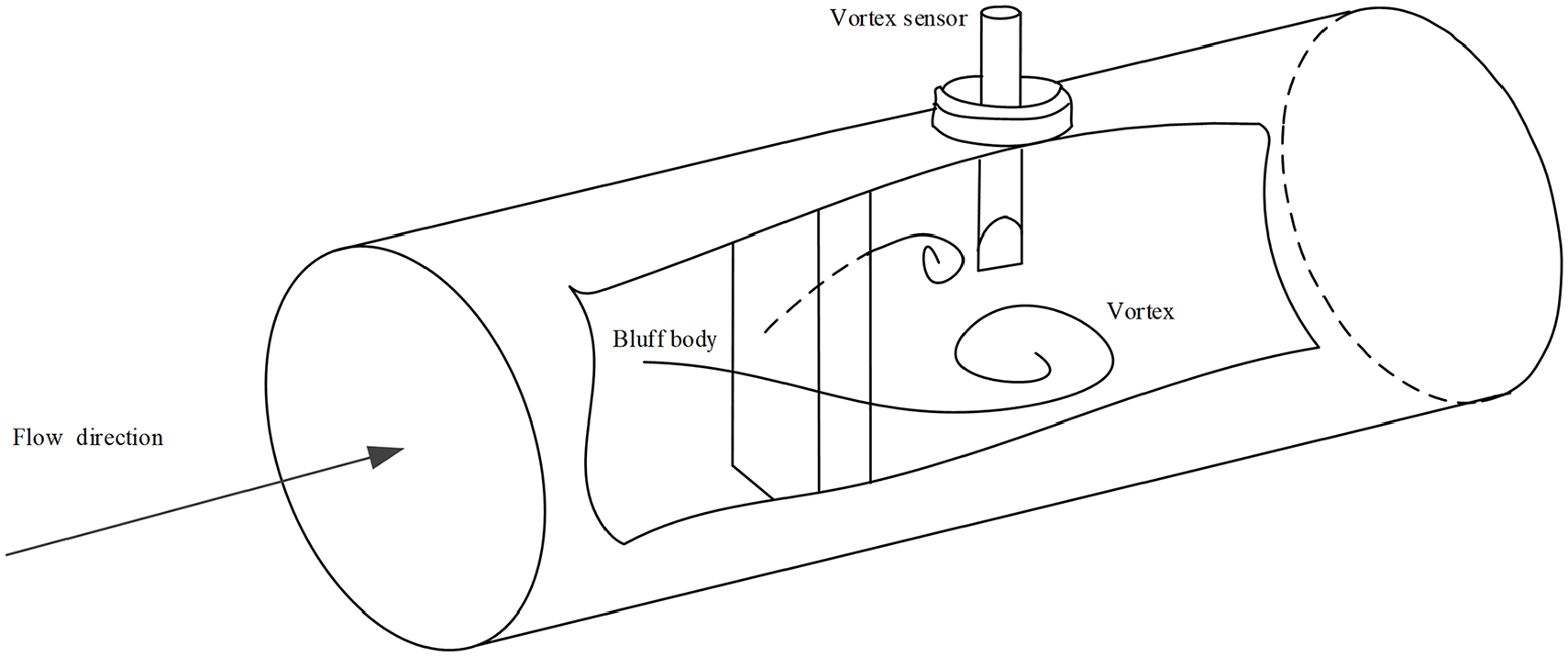
Kalman vortex flowmeter.

The frequency f of the vortex shedding is directly proportional to the flow rate Q_V. The relationship between them is given by

K_{m} = \frac{f}{Q_{V}}

(1)

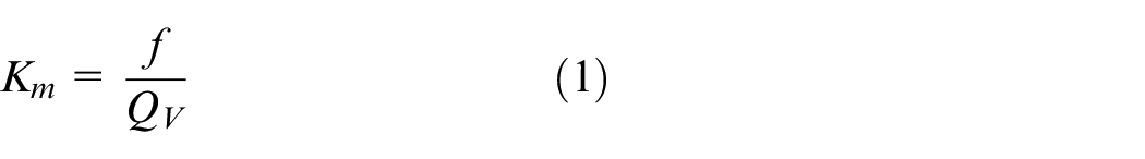
where K_m is the meter factor, and it is a constant when the structure of vortex meter is fixed.^2,3

Vortex flowmeter can effectively measure the flow velocity of various fluids such as gas, liquid and steam, meanwhile, it also has the following advantages: wide measurement range, low pressure loss and high precision, all of which makes it to be widely used around home and abroad.

The vortex flowmeter mainly measures the flow rate of the fluid according to the detachment frequency of the vortex street. In recent years, many scholars have proposed different processing methods for vortex street signals.

Chin-Chung Hu designed a digital filter to measure center frequency, which can be adjusted instantly with the magnitude of the input vortex signal. After passing through the digital filter, the signal enters the frequency calculation unit, which consists of two parts, fast Fourier transform (FFT) and autocorrelation algorithm. When the frequency of the signal exceeds 200 Hz, the frequency is calculated by the FFT, which can reduce the error caused by the frequency resolution during the operation. When the signal frequency is lower than 200 Hz, its frequency is calculated by an autocorrelation algorithm.⁴

To improve the anti-interference ability of the vortex flowmeter, Jiegang Peng and Min Fang⁵ proposed the Hilbert Huang transformation method to analyze the vortex signal to solve the problem that the piezoelectric sensor flowmeter is easily interfered by noise signal, Shao et al.⁶ proposed a method combining bilateral correction with weighted average on the basis of Fourier coefficients ratio, which can improve the anti-noise performance of the frequency correction.

To improve the accuracy of vortex flowmeter, Jinxia Li et al.⁷ proposed a signal processing algorithm based on empirical mode decomposition (EMD) and spectral center correction method (SCCM). In addition, a method of double window relaxing notch periodogram, which is capable of measuring the vortex frequency when the frequency band of noise and vortex frequency are in the same range, could also improve the accuracy of vortex flowmeter. In this method, the frequency and amplitude were estimated by Hanning and triangular window, respectively.⁸

The above vortex signal processing method mainly uses the FFT algorithm, which only requires the integer power of signal length of two. Some characteristics of the signal itself, such as the sparsity of the signal, are not taken into account. However, the frequency domain of signals commonly found in real life is always sparse, because most Fourier coefficients are small or equal to zero, such as image and speech signals.⁹ In that case, the Massachusetts Institute of Technology team gave the answer to whether we could find a faster algorithm to calculate the Fourier transform of such signals and they proposed an algorithm of digital signal processing called the sparse Fourier transform (SFT). Utilizing the sparsity of the signal frequency domain, the algorithm divides the Fourier coefficients of signal into “buckets” and then reconstructs the spectrum of the signal according to certain rules to change the longer discrete Fourier transform (DFT) operation into a shorter. Finally, the processing speed of the SFT algorithm is tens or even hundreds of times than that of FFT algorithm.⁹

In this paper, the SFT was applied to deal with the vortex street signal. And the noise signal is removed based on the amplitude–frequency characteristics of vortex signals. Our study confirms that this algorithm can ensure the high real-time performance and anti-interference ability of the system and the analysis speed is also greatly improved.

Main method

The spectrum of vortex flow signal is obtained by the SFT algorithm, and then the noise is filtered based on the amplitude–frequency characteristic of the vortex signal.

SFT

The precondition for the SFT algorithm is that the analyzed signal is sparse. Assuming that the discrete-time signal x(n) of length N is sparse and contains only K non-zero frequency components. The K is called the sparsity of the signal, and K is much smaller than N $(K << N)$ . The sparse signal x(n) can be expressed mathematically for

x (n) = \frac{1}{N} \sum_{k = 0}^{K - 1} X (k) e^{2 π jkn / N}, n \in Ω_{N}

(2)

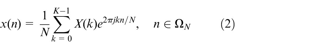
where Ω_N represents the set ${0, 1, \dots, N - 1}$ .

The key steps of the SFT algorithm are divided into spectrum premutation, window function, subsampled FFT and reconstruction. The main analysis process is shown in Figure 2.

Figure 2.

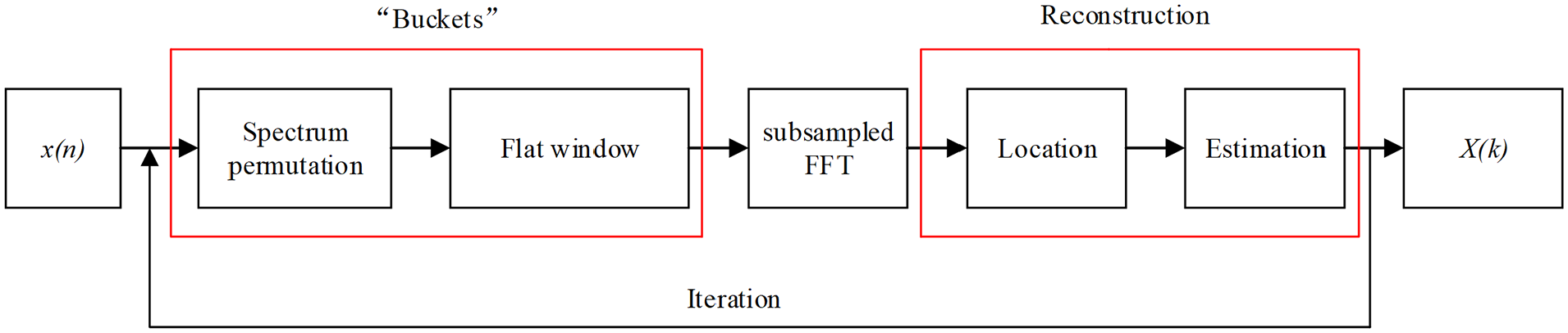
Flowchart of the SFT algorithm.

The purpose of the spectrum permutation is to uniformly distribute the large value points. When the Fourier coefficient of the signal is binned, the large value points need to be divided into different “buckets.” When two or more large-value frequency points are allocated to the same “bucket,” the coordinates and amplitude of the large-value frequency points cannot be solved. As the frequency domain cannot be permuted directly, the spectrum permutation can be achieved by remapping in the time domain. The transfer function is defined as $p_{σ, τ}$ , where σ is an odd number and the modulo operation on N is reversible, and the integer τ belongs to Ω_N

{(p_{σ, τ} x)}_{i} = x_{σ i + τ}

(3)

For ∀_a, the following formula is always true

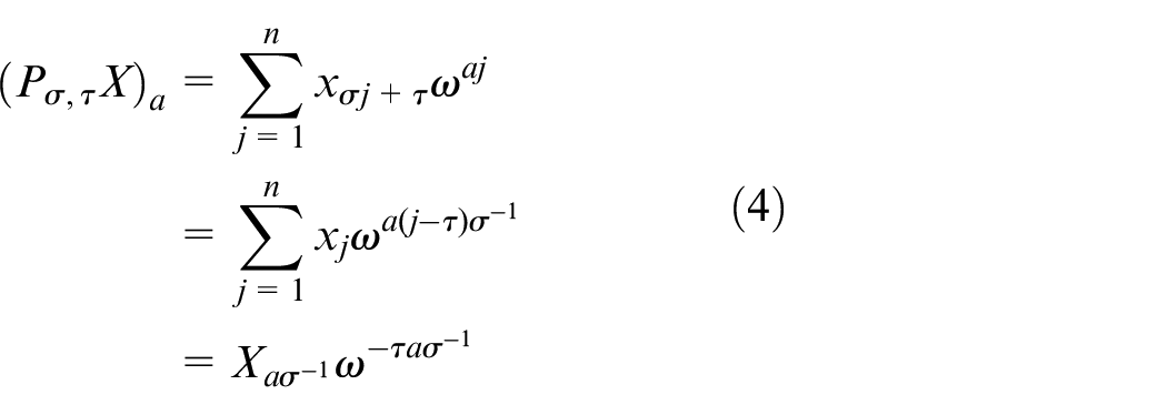
\begin{matrix} {(P_{σ, τ} X)}_{a} = \sum_{j = 1}^{n} x_{σ j + τ} ω^{aj} \\ = \sum_{j = 1}^{n} x_{j} ω^{a (j - τ) σ^{- 1}} \\ = X_{a σ^{- 1}} ω^{- τ a σ^{- 1}} \end{matrix}

(4)

Therefore, the formula for changing the frequency domain after the time domain is rearranged as

{(P_{σ, τ} X)}_{σ i} = X_{i} ω^{- τ i}

(5)

where ω equals $e^{2 π i / n}$ .

To ensure the efficiency of the algorithm and prevent spectral leakage, it is necessary to design a filter with concentrated energy in both time and frequency domains. According to the literature,¹⁰ the flat window function is a convolution of the Sinc window function with the Gaussian window function. As shown in Figure 3, the frequency response of the filter G is nearly flat in the passband and exponentially decays in the stopband. This ensures that the spectral leakage between adjacent large value frequencies is negligible. This characteristic of the flat window function allows the energy of the filter to be concentrated in both the time and frequency domains.

Figure 3.

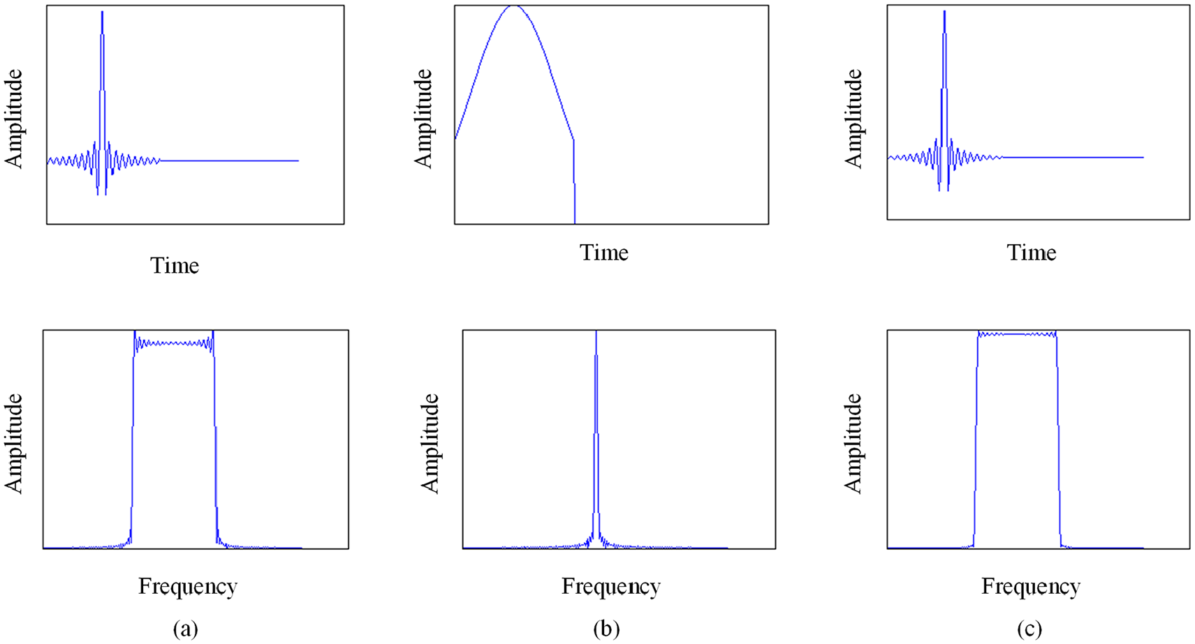
The images of window function time domain and frequency: (a) Sinc window function, (b) Gaussian window function and (c) flat window function.

If you want to subsample the signal frequency domain at equal intervals N/B, you need to make parameter B divide N, that is

Z (k) = X (\frac{kN}{B}), k \in Ω_{B}

(6)

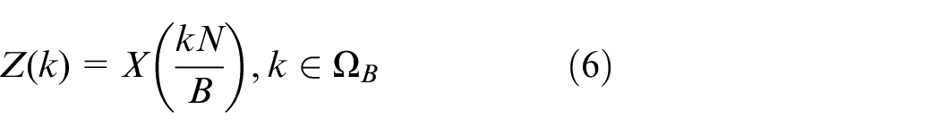
It proves that Z(k) is the result of the DFT after the original signal aliasing

z (n) = \sum_{j = 0}^{N / B - 1} x (n + Bj), n \in Ω_{B}

(7)

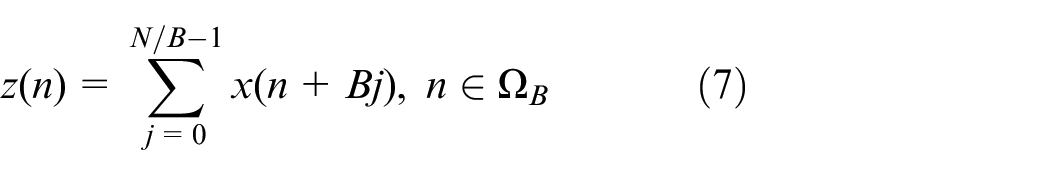
After aliasing, the frequency domain spectrum is reduced from N to B. This is the key reason why the complexity of the SFT algorithm is lower than the FFT algorithm.

Define the “hash function” $h_{σ} : h_{σ} (k) = round (σ \cdot k \cdot N / B)$ , mapping each point in $Ω_{N}$ to $Ω_{B}$ . Define the “offset” $o_{σ} : o_{σ} (k) = σ \cdot k - h_{σ} (k) \cdot (N / B)$ ; Define the set J, which contains the coordinates k of K larger magnitudes in Z(k). $I_{r}$ is obtained by hashing inverse mapping, that is, $I_{r} = {k \in [0, N - 1] | h_{σ} (k) \in J}$ . Finally, the K large-value points are taken out to estimate the frequency of the original signal. This step is called a location loop.

For each $k \in I_{r}$ , $X' (k) = Z (h_{σ} (k)) ω^{- τ k} / G (o_{σ} (k))$ is used as the corresponding frequency estimate. Each location cycle obtains a coordinate set $I_{r}$ . In the $L = O (\log_{2} N)$ cycle, any coordinate $k \in I = I_{1} \cup \dots \cup I_{r}$ , if the number of occurrences is greater than L/2, then it is classified into the set $I'$ , and it is considered that the set $I'$ contains all of the target frequency coordinates.

For each $k \in I'$ , the median value of $X_{r} (k)$ obtained for each cycle is taken as the final frequency estimation value, that is, $X (k) = m edian ({X_{r} (k) | r \in {1, \dots, L}}) .$

Amplitude–frequency characteristics of the vortex signal

Within a certain range, the vortex signal amplitude A has the following relationship with the vortex frequency f

A \propto ρ D^{2} f^{2}

(8)

where $ρ$ is the density of the fluid medium and $D$ is the pipe diameter.¹¹

When the pipe diameter D and the fluid density are constant, the output amplitude of the vortex sensor is proportional to $f^{2}$ . The relationship between amplitude A and frequency square $f^{2}$ can also be measured experimentally. Considering that the actual vortex measurement system cannot achieve full cycle sampling for the unknown output signal, we adopted the Hanning window interpolation method¹² to correct the spectrum to minimize the effects of non-full cycle and fence effect.

The vortex signal waveform and a corrected spectrum of the sensor output at a different flow rates were shown in Figure 4. This experiment takes a 50-mm diameter gas vortex flowmeter as an example. At each flow point, the data collected by the oscilloscope are divided into five groups, each group of 2048 data. Then, the frequency and amplitude of the signals were obtained by spectrum analysis. The frequency and amplitude at each flow point were averaged, and then the averaged amplitude and frequency of vortex signal were curve fitted. The results were shown in Figure 5.

Figure 4.

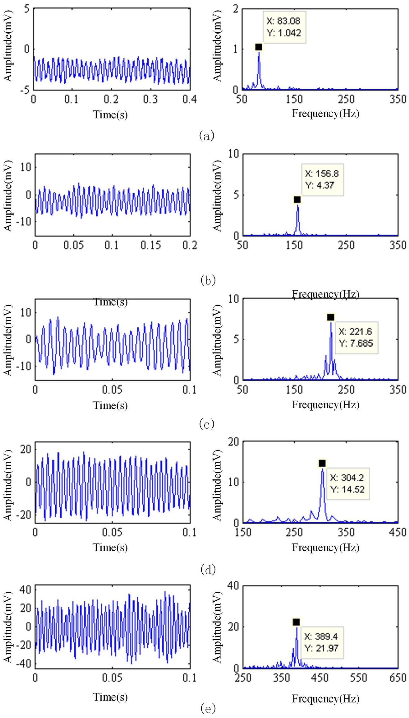
Time and frequency-domain at different flow rates: (a) Q_V = 30 m³ h⁻1, (b) Q_V = 60 m³ h⁻1, (c) Q_V = 90 m³ h⁻1, (d) Q_V = 120 m³ h⁻1 and (e) Q_V = 160 m3 h⁻1.

Figure 5.

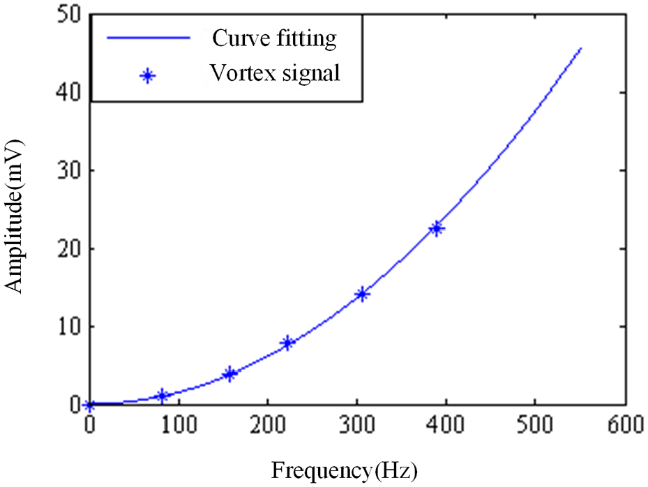
Amplitude–frequency relationship.

The fitting equation in the above figure is

A = 1.5 \times 10^{- 4} f^{2}

(9)

It can be seen from Figure 5 that the quadratic curve fitting of the amplitude and frequency relationship of the vortex signal can be better achieved by the least square method.

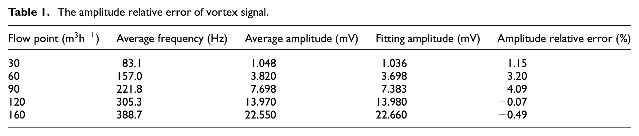
In the above experiment, the relative error between the average amplitude of vortex signal and the corresponding point amplitude on the fitted curve is shown in Table 1. It can be seen from Figure 5 that the actual vortex signal amplitude fluctuates around the theoretical value, and Table 1 also shows that the amplitude fluctuation of the vortex signal has a certain range. The more suitable expression for the amplitude–frequency relationship is as follows

A = c (1 \pm δ) f^{2}

(10)

where c is the coefficient and δ is the relative error limit. The theoretical fit curve and the threshold curve of the amplitude–frequency relationship were shown in Figure 6. The solid line is the theoretical fit curve of the amplitude–frequency relationship, and the dashed line is the threshold curve of the amplitude fluctuation. Table 1 shows the average amplitude fluctuates in the fitted curve, ranging from −0.47% to 4.09%. But considering that the actual working condition is more severe than the experimental environment, the relative error of the vortex signal amplitude fluctuation is 10%.

Table 1.

The amplitude relative error of vortex signal.

Flow point $(m^{3} h^{- 1})$	Average frequency (Hz)	Average amplitude (mV)	Fitting amplitude (mV)	Amplitude relative error (%)
30	83.1	1.048	1.036	1.15
60	157.0	3.820	3.698	3.20
90	221.8	7.698	7.383	4.09
120	305.3	13.970	13.980	−0.07
160	388.7	22.550	22.660	−0.49

Figure 6.

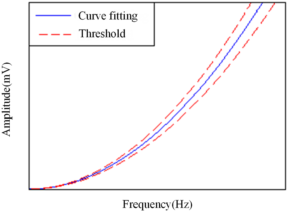
The theoretical fit curve and the threshold curve of the amplitude–frequency relationship.

Results and discussions

The vortex signal analyzed in this paper is obtained from the pipeline vibration signal. The number of sampling points is 2048 and the data are analyzed by the SFT.

Figure 7 shows a spectrogram obtained by analyzing the vortex time domain signal. As shown in Figure 7, the number of higher frequency points is small, and the rest is mostly 0, which satisfies the sparsity of the signal.

Figure 7.

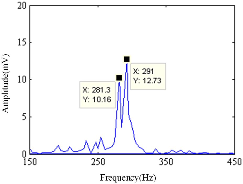
Frequency-domain signal, Q_V = 120 m³ h⁻¹.

When the SFT algorithm is used to recover the signal spectrum, the obtained spectrum information is that the frequency coordinates of large-value are k1 = 283.1 Hz, k2 = 291 Hz, and the corresponding amplitudes are X(k1) = 10.23 mV, X(k2) = 12.89 mV. The magnitude of the remaining frequency points can be approximately equal to zero, so the sparsity K is taken as 2. 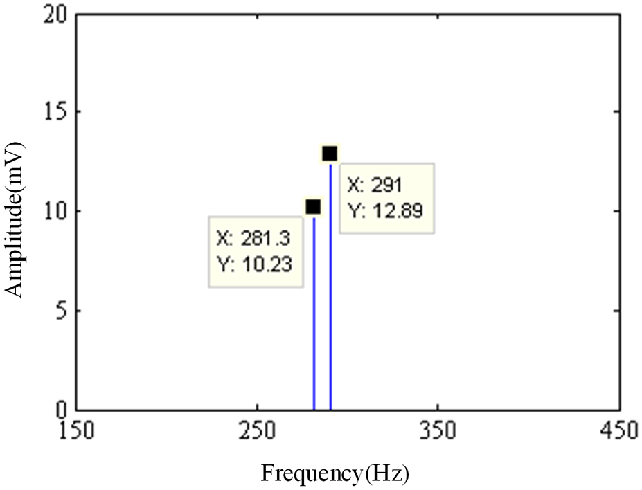Specifically, to improve the performance of the algorithm, we use $B \approx \sqrt{NK}$ .¹⁰ It can be seen from Figure 7 that the two largest amplitudes calculated by the FFT algorithm are Y(k1) = 10.16 mV, Y(k2) = 12.73 mV. The recovered signal spectrum is shown in Figure 8. It can be seen from the comparison between Figures 7 and 8, the FFT algorithm calculates the amplitudes of all the frequency points of the signal spectrum, while the SFT algorithm only calculates the frequency coordinates and amplitude of the K large-value frequencies. The remaining frequency points are all set to 0.

Figure 8.

The vortex signal spectrum recovered by SFT algorithm, Q_V = 120 m³ h⁻¹.

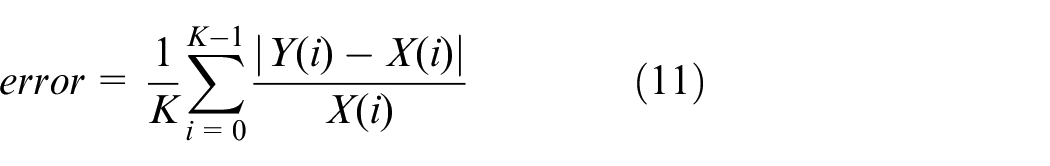
In addition, the large-value frequency coordinates recovered by the SFT algorithm are the same as the large-frequency coordinates of the signal spectrum obtained by the FFT. Meanwhile, the relative errors of the amplitudes of the coordinate points k1, k2 calculated by FFT and SFT are −0.68%, −1.24%, respectively. The vortex signal of Figure 4 is recovered using the SFT algorithm, and the error results are shown in Table 2. The expression of the overall error of the SFT algorithm to recover the frequency point is as follows

error = \frac{1}{K} \sum_{i = 0}^{K - 1} \frac{| Y (i) - X (i) |}{X (i)}

(11)

Table 2.

Recovery spectrum error table.

Flow point $(m^{3} h^{- 1})$	Amplitude (FFT) (mV)	Amplitude (SFT) (mV)	Amplitude error (%)
30	1.042	1.059	−1.60
60	4.370	4.423	−1.19
90	7.685	7.697	−0.15
120	14.520	14.576	−0.38
160	21.970	22.053	−0.37

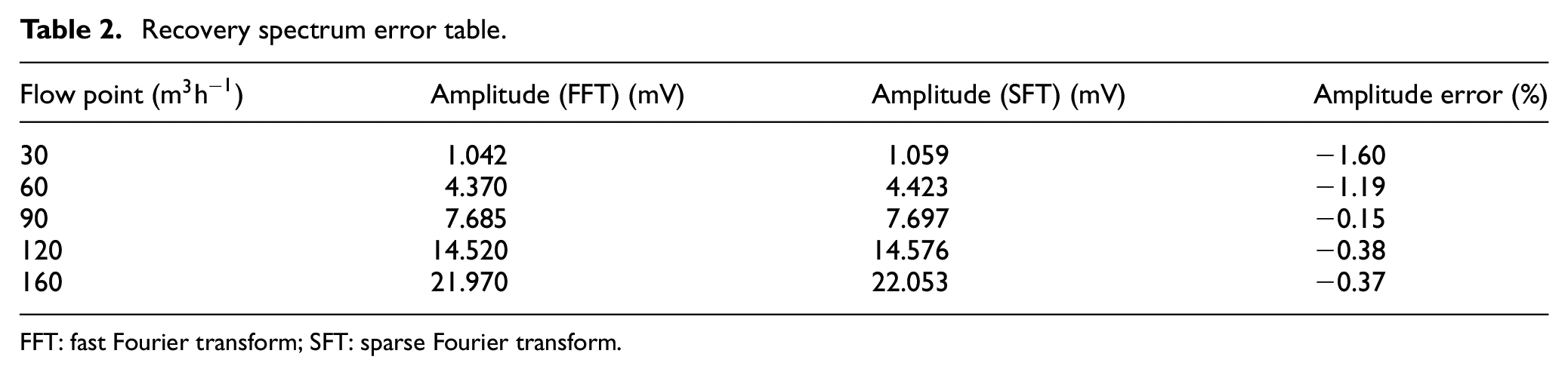
FFT: fast Fourier transform; SFT: sparse Fourier transform.

The error is equal to 0.96%. The results indicate that the SFT algorithm can recover the spectrum of the signal very well.

Figure 9 shows that it is possible to discriminate whether the data obtained by the SFT is a noise signal or a vortex signal by the amplitude–frequency characteristic relationship. The amplitude–frequency characteristic relationship can identify the vortex signal from the mixed signal containing vibration noise, thereby achieving the purpose of improving the anti-vibration performance of the vortex flowmeter.

Figure 9.

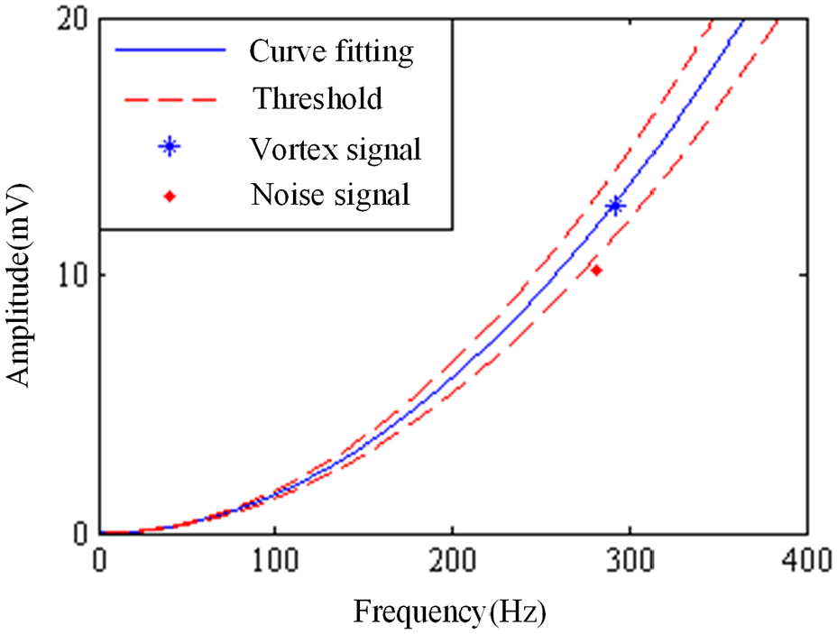
Vortex signal identified by the amplitude–frequency relationship.

The superiority of the SFT algorithm will be analyzed as follows. The time complexity of the SFT algorithm based on hash map is $O (\sqrt{NKlo g_{2} N} lo g_{2} N)$ , while the FFT algorithm is $O (Nlo g_{2} N)$ . With the signal length N increases, the time complexity of the SFT and FFT will be changed accordingly. The order of magnitude of time complexity will be used to characterize this change

\frac{\sqrt{NK \log_{2} N \log_{2} N}}{N \log_{2} N} = \sqrt{\frac{K \log_{2} N}{N}}

(12)

When the sparsity K takes different values, the ratio of the time complexity of the SFT to the FFT is shown in Figure 10. When K is 4, 8 and 16, the ratio is 0.147, 0.207, 0.293, correspondingly. It can be seen that, in the case where other parameters are fixed, the time complexity of the SFT algorithm becomes larger as the value of the sparsity K increases.

Figure 10.

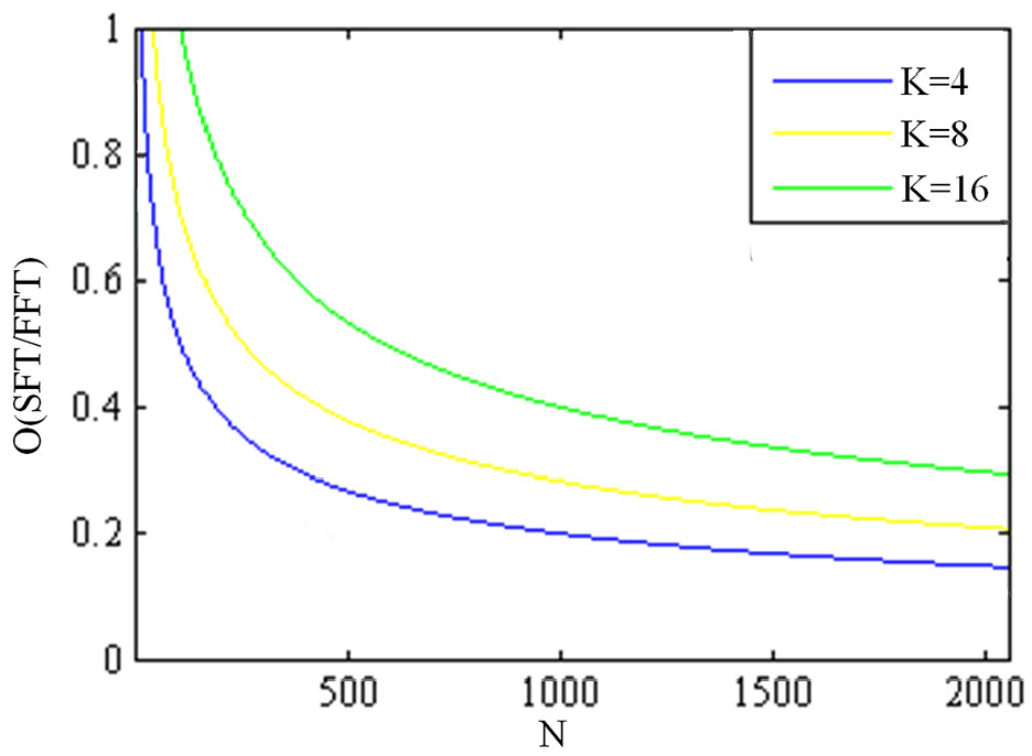
Ratio curve of time complexity between SFT and FFT.

Comparisons with other methods

In Jinxia Li’s¹³ study, the piezoelectric sensor signals were denoised based on the EMD combined with autocorrelation function decay. After denoising, the SCCM was developed to correct the result of FFT, which is based on the window energy property of the power spectrum. The flowchart is shown in Figure 11. For comparison with Li’s method, this method was used to process our vortex signal, and the corrected frequency is shown in Figure 12.

Figure 11.

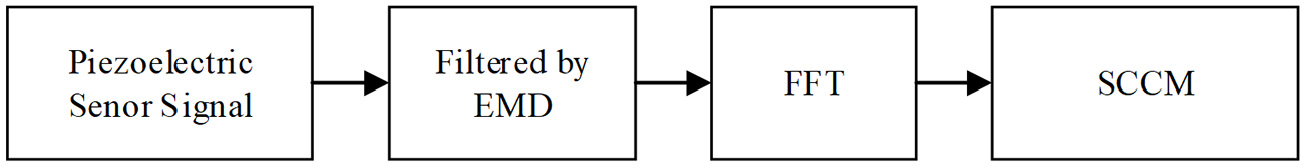
The flowchart of Li’s study.

Figure 12.

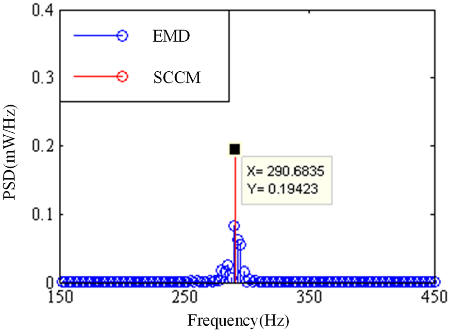
The results of EMD and SCCM, Q_V = 120 m³ h⁻¹.

In our study, the frequency of the vortex signal was first calculated by the SFT. Then, the amplitude–frequency characteristic relationship was developed to remove noise from the signal.¹⁴ As shown in Figures 8 and 12, the vortex signal frequencies obtained by the two methods are 291 and 290.6835 Hz. The results show that the frequency obtained by our method is more accurate. In Li’s research, the frequency of the vortex signal after denoising was obtained by FFT. Then, the frequency correction method is used to obtain a more accurate frequency. Considering the superiority of the SFT algorithm, our method has better real-time performance. The length and sparsity of the vortex signal are 2048 and 2, respectively. It can be seen from Figure 13 that when parameter K is equal to 2, as the number of sampling points N increases, the ratio of the time complexity of the SFT algorithm to the FFT algorithm becomes smaller and smaller. When the number of vortex signal sampling points is 2048, the time complexity of the SFT algorithm is only 10.36% of the FFT algorithm.

Figure 13.

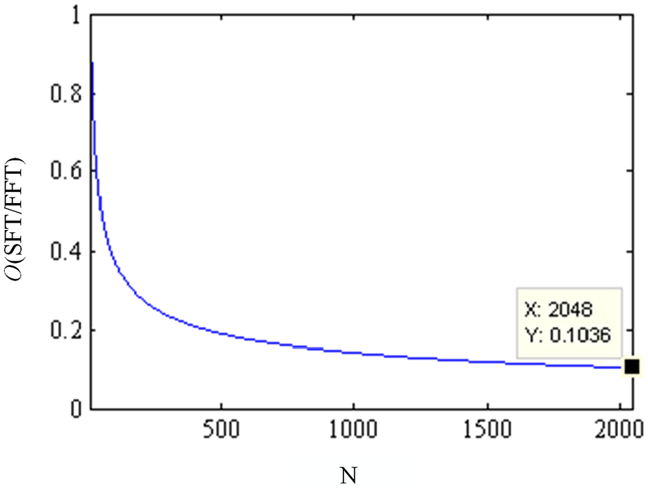
Ratio curve of time complexity between SFT and FFT (K =2, N = 2048).

Conclusion

In this paper, the measurement of the vortex frequency of the gas is based on a method that combines SFT algorithm and the amplitude–frequency characteristic of the vortex signal. The results indicated that this method can effectively reduce the noise signal, accelerate the processing speed of vortex signals and improve the real-time performance of the system.

Footnotes

Declaration of conflicting interests

The author(s) declared no potential conflicts of interest with respect to the research, authorship and/or publication of this article.

Funding

The author(s) disclosed receipt of the following financial support for the research, authorship, and/or publication of this article: This work is supported by Key Project of Science and Technology Commission of Shanghai Municipality under Grant No. 16010500300.

ORCID iDs

Jie Chen

Yun Cao

Bin Li

References

Zhang

Huang

Sun

A study of mass flow rate measurement based on the vortex shedding principle. Flow Meas Instrume 2006; 17(1): 29–38.

Dijstelbergen

HH.

The performance of a swirl flowmeter. J Phys E: Sci Instrum 1970; 3(11): 886–888.

TT.

Investigation on the fluid motion in precession type swirl flowmeter. Nung yeh chi hsieh hsueh pao. = Acta agromechanica sinica 1979; 10: 36–46.

Miau

Chen

Determination of real-time vortex shedding frequency by a DSP. J Chin Soc Mech Eng 2006; 27(3): 335–342.

Peng

Fang

Response of a dual triangulate bluff body vortex flowmeter to oscillatory flow. Flow Meas Instrum 2014; 35: 16–27.

Shao

Shu

, et al. A frequency correcting method combining bilateral correction with weighted average for vortex flow sensor signal. In: IEEE transactions on instrumentation and measurement, 4 July 2017, pp. 2711–2724. New York: IEEE, https://ieeexplore.ieee.org/document/7968350

Wang

Ding

, et al. EMD and spectrum-centrobaric- correction-based analysis of vortex street characteristics in mist annular flow of wet gas. IEEE Trans Instrum Meas 2018; 67(5): 1150–1160.

Zheng

Zhang

Research on vortex signal processing based on double-window relaxing notch periodogram. Flow Meas Instrum 2008; 19(2): 85–91.

Hassanieh

Indyk

Katabi

, et al. Nearly optimal sparse Fourier transform, 2012, https://arxiv.org/abs/1201.2501

10.

Hassanieh

Indyk

Katabi

, et al. Simple and practical algorithm for sparse Fourier transform. In: Proceedings of the twenty-third annual ACM-SIAM symposium on discrete algorithms, 2012, pp. 1183–1194. Philadelphia, PA: Society for Industrial and Applied Mathematics, https://groups.csail.mit.edu/netmit/sFFT/soda_paper.pdf

11.

Chen

Dai

. Vortex signal processing method based on flow momentum. In: 2009 9th international conference on electronic measurement & instruments, Beijing, China, 16–19 August 2009, pp. 4–450. New York: IEEE.

12.

Grandke

Interpolation algorithms for discrete Fourier transforms of weighted signals. IEEE Trans Instrum Meas 1983; 32(2): 350–355.

13.

Wang

Ding

, et al. Emd and spectrum-centrobaric-correction-based analysis of vortex street characteristics in mist annular flow of wet gas. IEEE Trans Instrum Meas 2018; PP(99): 1–11.

14.

Chen

Fan

, et al. Novel algorithm of tracking band-pass digital filter with amplitude 1/f2 attenuation for vortex signal extraction. Flow Meas Instrum 2015; 45: 82–92.

Sparse Fourier transform and amplitude–frequency characteristics analysis of vortex street signal

Abstract

Keywords

Introduction

Main method

SFT

Amplitude–frequency characteristics of the vortex signal

Results and discussions

Comparisons with other methods

Conclusion

Footnotes

Declaration of conflicting interests

Funding

ORCID iDs

References