Mode Inference using enhanced Segmentation and Pre-processing on raw Global Positioning System data

Abstract

Many applications use the Global Positioning System data that provide rich context information for multiple purposes. Easier availability and access of Global Positioning System data can facilitate various mobile applications, and one of such applications is to infer the mobility of a user. Most existing works for inferring users’ transportation modes need the combination of Global Positioning System data and other types of data such as accelerometer and Global System for Mobile Communications. However, the dependency of the applications to use data sources other than the Global Positioning System makes the use of application difficult if peer data source is not available. In this paper, we introduce a new generic framework for the inference of transportation mode by only using the Global Positioning System data. Our contribution is threefold. First, we propose a new method for Global Positioning System trajectory data preprocessing using grid probability distribution function. Second, we introduce an algorithm for the change point–based trajectory segmentation, to more effectively identify the single-mode segments from Global Positioning System trajectories. Third, we introduce new statistical-based topographic features that are more discriminative for transportation mode detection. Through extensive evaluation on the large trajectory data GeoLife, our approach shows significant performance improvement in terms of accuracy over state-of-the-art baseline models.

Introduction

Understanding the mobility patterns of a user by analyzing the Global Positioning System (GPS) trajectory data is an important research problem, providing the rich context information that can be utilized for traffic management and city transport planning.^1,2 Transportation experts can develop the strategies to reduce traffic congestion, air pollution, cost and time for people based on the inference of transportation modes from GPS trajectories, and thus the existing transportation system can be improved.^3–5 A GPS trajectory is a path of GPS points generated in sequence by any moving object. Each GPS point can be represented by a tuple (x, y, t), where x, y and t are latitude, longitude and timestamp of a GPS point, respectively. ⁶ Transportation mode inference aims to infer modes of transport of a user from the user’s data obtained through multiple sensor types including accelerometer, Global System for Mobile Communications (GSM) or GPS sensors. Learning the transportation modes such as walk, bike, bus and car from trajectory data is of great significance for both the users and service providers, because the learned user’s behaviors can be used in many applications for multiple purposes like flow prediction^7,8 traffic congestion^9,10 etc.. From the perspective of users, it can help in understanding life patterns and the social patterns of the users to facilitate life-sharing experiences among the users.^11–13 It is also useful for personalized recommendations and to provide intelligent services in travel behavior research field. ¹⁴ It also provides the intelligent services assisting the wide range of behavioral applications, which includes finding the routes to the destinations, extracting traffic conditions, location-based activity recognition, intelligent surveillance systems and many more. ¹⁵ Transport companies can make the planning to reduce travel time and cost, and to encounter the traffic congestion and air pollution.

Travel mode information were traditionally collected in the past through questionnaires and telephone surveys, and thus such methods were slow, inconvenient, inaccurate and expensive, resulting in a low response rate and imperfect information^3,14 Coarse and fine-grained data were used for the purpose of activity recognition; the performance is higher when using the fine-grained sensors like the cluster of wearable sensors, but carrying such devices was not feasible. Radio signal technologies like GSM and Wi-Fi although do not involve the human cost, but due to coarse-grained data in nature, only simple movement types like stationary or moving could be detected. ¹⁶ This requires cost-effective technologies, such as GPS, which can collect fine-grained travel data while reducing laborious and time-consuming tasks. The advantage of handheld devices is that they can easily produce large amount of GPS trajectories. ⁴

Recent studies in the last decade try to infer transportation modes from GPS trajectories. Zheng et. al. ⁷ proposed a framework that first partitioned the trajectory into single-mode segments using change point–based segmentation algorithm and then classified the segments using features obtained from the segments. Several studies^17–19 identified different modes of transportation using both Geographic Information System (GIS) information and GPS data. Zhu et al. ²⁰ introduced some new features and segmentation algorithms. Dabiri and Heaslip ³ and Endo ²¹ used features obtained from fixed-length segments to feed into convolution neural networks. The limitations of these studies are that they use either the GIS data that usually are not available for all the places or segmentation algorithms that cannot handle the noisy data. Deep neural network (DNN)-based frameworks^21,22 are slower and also use the fixed-length segments that do not perform better in all cases. DNN architectures are also dependent on sufficient and informative training data^23–25 and exclude potentially useful hand-designed features.

Only using GPS data to infer transportation mode is more general and portable, but it also makes the problem more challenging ¹⁶ due to the following reasons. First, as only GPS data are available, it is difficult to extract sufficient discriminative features for the studied problem. Second, it is also difficult to identify the change points of the transportation modes to partition the trajectory data without the help of other information such as GIS. GPS-enabled handheld devices can produce only the spatiotemporal features without any explicit information about the use of transportation modes. This requires new data processing, representation and mining techniques to correctly classify the modes of transport using raw GPS data.^3,26 Velocity-based recognition methods based on simple rules are far from enough to solve this problem. The characteristics of different modes of transportation are often susceptible to weather and traffic conditions. In the scenario of traffic congestion, the average velocity of car is as slow as walk, and during rain, the behavior of a bus is similar to a bicycle in the terms of velocity. ¹¹ Therefore, when a user takes multiple modes of transportation during a trip, it becomes more difficult to identify the transportation modes from GPS trajectories. Therefore, a new method is needed to automatically and accurately infer the mode of transport and the transition between them from raw GPS data.

The paper proposes an enhanced transportation mode inference technique that only uses the GPS data to classify four different types of transportation modes including walk, bike, bus and car. Specifically, we first present a new way of data preprocessing by computing grid probability distribution function. Furthermore, a new algorithm for trajectory segmentation is proposed using enhanced algorithm to divide a trip into multiple segments. Besides the motion-based features, we also introduce some new probabilistic features based on grid probability distribution function to help identify the probabilities of transportation modes prior to classification. Our approach is different from all other existing approaches, as we made the comparison based on correctly identified distances covered by correctly identified segment; because lengths of all segments are different, so this is more objective, ¹⁶ whereas existing works only evaluate on number of segments correctly identified.

The core contributions of the work lie in that

• We proposed a new framework to infer the modes of transport from only raw GPS trajectory data using a new data preprocessing methodology and the segmentation approach.

• We propose a novel approach of probabilistic-based grid system for the representation of GPS trajectories, for identifying spatial probability distributions of transportation modes for a region.

• We propose a new segmentation algorithm to identify the change points of the transportation modes in GPS trajectories and extract single-mode segments for classification purpose.

• We extract the new features set from identified segments such as probabilities of the transportation modes prior to classification task, weekday type and interquartile mean of velocity and acceleration that proved to be more robust with higher prediction accuracy.

The rest of this paper is organized as follows. First, in section “Related work,” we give a brief survey on the related work. We set out details of our framework in section “Methodology,” including the data preprocessing steps, trajectory segmentation and classification models. In section “Experiments,” we present the results of our methodology and evaluate our proposed model. Finally, we conclude the paper in section “Conclusion.”

Related work

This section gives a brief overview of the work done under the field of transportation modes classification. In recent years, mobile phones equipped with the GPS technology, collecting the user’s GPS traces, have become very convenient and allow to infer the transport mode from the GPS trajectories.^27,28 Compared with other GPS-enabled devices, the main advantage of handheld devices is that they can easily produce GPS trajectories. ⁴ As a result, this dominant region-wide sensing technology can generate a large number of vehicle, human and biological trajectory data. Numerous studies have attempted to use various data sources including GPS, GSM and accelerometer that were collected by different types of sensors to detect transport patterns. Zheng and colleagues^11,16 use GPS data to classify four classes of transportation modes. Some studies also tried to use GSM data ²⁹ and accelerometer data ³⁰ to identify the transportation modes. In addition, some mobility detection studies have integrated data from multiple data sources to improve the classification results. Similarly, some studies^28,31,32 exploited accelerometer information with GPS data for the inference of transportation modes that achieved better results over GPS-only methods. Earlier studies^30,32–34 achieved better results using accelerometer data obtained through mobile phones to identify the transport modes of a user. In some other studies, Pärkkä et al. ³⁵ used the features heart rate, light intensity and body temperature obtained through other sensor types for the activity recognition of a user including walking, boating, cycling and running. Although using multiple sensor data may lead to better results, a method using a single source of the data may be more practical because accessing data from multiple sources is not always possible.^3,14

Over the past decade, many studies inferred the mobility patterns with the support of GIS information using machine learning methods and achieved significant results,^36–38 but there are certain limitations in their work. The performance of their work improved either using more sensors or to integrate GIS features with the GPS data. GIS information is very helpful to identify more discriminative features as given in previous works.^17,18 These studies use GPS data with GIS information for the classification of transportation modes. For example, Liang et al. ¹⁸ took the bus stop information from open street maps to integrate with the GPS data and increased the overall classification results as compared to GPS-only data. All of these methods mentioned above have the constraint to be dependent on the use of multiple sensor’s data or the use of GIS data to produce more exciting features that can enhance the accuracy of the system, but it is not possible to keep multiple sensors with them all the time and in most of occasions access to GIS information is not possible in many cities. ³⁹ Transport mode inference using only raw GPS data is a big challenge, so it is necessary to identify more robust and discriminative features within the GPS data to identify multiple types of transportation modes of a user from GPS trajectories.

The general processing steps are used to divide the GPS trajectory separated by transition points into the sequence of segments called segmentation, representing a transition of a transport mode from one segment to the next segment. ⁴⁰ The accuracy of the extraction of correct transition points also affects the accuracy of the identification of transportation modes. ²⁰ Earlier studies try to find the transition points based on acceleration data obtained through accelerometer; few studies take support of geographical information of roads, bus stops and parking lots for the same purpose. Existing methods using geographical data cannot be used widely because it increases the cost, complexity and computational overhead. Zheng et al. ¹¹ used the threshold velocity and acceleration to identify the walking segment and consider the start and end points of walk segments as change points. Zhu et al. ²⁰ identified the transition points based on the concept that it appears in a situation of sudden change in velocity; they identified the walk segments continuing for 90 s and 50 m threshold values for time and distance. Xiao et al. ⁴¹ identified the first and last points of the walk segment as transition points larger than the threshold of 60 s and extracted the walk segment from the GPS trajectory through a number of rules related to the time and velocity characteristics. Liang et al. ¹⁸ introduced new approach to segment the trajectory based on stay points. All these algorithms have deficiency that it causes performance degradation during segment merging in case of noise in the data.

Transportation mode of a user is one of the fundamental properties of human mobility and a hot research topic.^1,22 A user can take multiple types of transportation modes in his or her daily life, for example, walk, bike, car, bus, train, boat and subway. These modes can be classified through its velocities in normal conditions, but it becomes more difficult when multiple modes have to be identified in a single trip, because motion-based features are sensitive to weather conditions or traffic congestion on the roads. In addition to motion features, Zheng et al.^11,16,42 introduced the new behavioral features like the rate of heading change and stop rate that are more robust for the identification of transportation modes using supervised learning methods. Most of the studies for the classification of mobility modes used GPS data involving machine learning methods such as k-nearest neighbor (kNN), support vector machine (SVM) and decision tree (DT). In addition to statistical methods, random subspace methods and DNNs were also used for this problem, ¹⁴ but none of these methods always achieve best accuracy in all cases. Therefore, choosing the machine learning method is not always a criterion to achieve best accuracy, but other important factors are also important including modeling of the data and extracting the most representative features for classification.

Identification of the more discriminative features is the key component to transportation mode detection. ¹⁸ Feature selection is an important step in applying advanced classification methods for transportation mode detection. Appropriate features can significantly improve the detection accuracy of the algorithm and reduce the algorithm complexity. ⁴³ Most of previous studies^9,40 used variety of statistical features related to velocity and accelerations of transportation modes like mean velocity, expectation of velocity and acceleration, top 3 velocities and accelerations. Zheng et al. ¹⁶ proposed three new features that are tolerant to traffic conditions, that is, stop rate, velocity change and heading change rates. Zhu et al. ²⁰ introduced two new features, time slice type and acceleration change rate, to further improve the performance of algorithm. New features are proposed in addition to above features that are more discriminative in identifying the transportation modes from GPS data. Details of new proposed features will be explained in section “Methodology.”

Methodology

In this section, we will first define the terminologies related to our problem, and then we will explain our four-step framework including data preprocessing, segmentation, feature extraction and inference for the identification of transportation modes. Following are few terminologies used in our paper for the identification of transportation modes:

• Transportation Mode (M). This is a way used to travel the distance, for example, walk, bike, bus or car.

• Trajectory (T). A trajectory is a sequence of connected GPS points. A trajectory is divided into multiple trips (r) based on time threshold value.

• Trip (R). A single trip R consists of multiple GPS points. Each GPS point is a tuple consisting of latitude, longitude and timestamp value. More than one transportation modes can exist in a trip.

• Segment (S). A segment represents the single unit of a trip R and it contains one and only one transportation mode M. A single trip R consists of multiple segments S.

• Change point (C). A change point C is a location, where user switched his transportation mode M.

Problem definition

Given a trajectory T, our goal is to identify trip R, change point C and segment S, then infer the hybrid transportation mode M of a user, using our new proposed supervised learning framework MoISP (Mode Inference using enhanced Segmentation algorithm and Pre-processing) on raw GPS data.

Framework

In this section, we briefly introduced the proposed framework MoISP. Figure 1 shows the architecture of MoISP. Highlighted parts in Figure 1 are components where our core contributions are involved. The framework takes GPS trajectories as input, which are obtained through multiple GPS sensors over a period of time. The first step is preprocessing of GPS trajectories, in which we remove all outlier points and represent the data in two-dimensional (2D) grid. Then, point-level features are calculated and passed to segmentation algorithm to partition the trajectories. Probability distribution function is also calculated to identify probabilistic features of the segments. Next step is the trajectory segmentation. Each trip is divided into segments based on switching the transportation mode, and each segment consists of one and only one transportation mode. Then, segment-level features are extracted as a feature vector. Finally, the inference model takes feature vector as input and classifies the transportation modes of the GPS trajectories.

Figure 1.

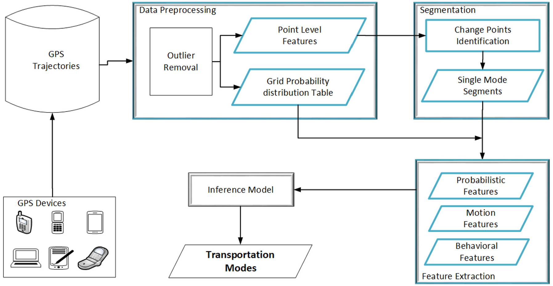
Framework of MoISP.

Data preprocessing

We use two consecutive GPS points to calculate the motion characteristics of each GPS point. Outlier detection is an important task as user may mislabel the trajectory by mistake. A walk segment may be given label as car, so it impacts overall descriptive statistical measures of different transportation modes. In our work, we first calculate some point-level features such as distance, time, velocity, acceleration, jerk and bearing previously used by Dabiri and Heaslip. ³ Second, we remove the duplicate GPS points that are logged multiple times because of the device error and outlier GPS points, belonging to transportation modes that exceed the maximum allowable velocities and accelerations given in the work. ³

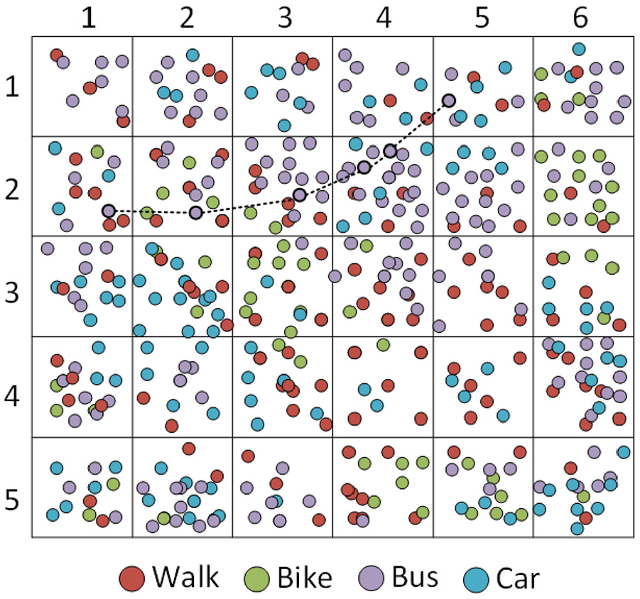
We also create grid probability distribution table that is used to calculate probabilistic features in feature extraction module. It will work as follows. First, the geographical space is divided into 2D grid and each cell of a grid corresponds to a specific row and column as shown in Figure 2. For simplicity, the 2D grid index is converted to unidimensional grid index using equation (1)

$$i=\mathrm{grid}\_\mathrm{index}=(\mathrm{row}-1)\times \mathrm{cols}+\mathrm{col}$$

(1)

where row and col represent the row and column IDs of a 2D grid, and cols is the total number of columns of a 2D grid.

Figure 2.

Grid indexing of geographical space.

Each grid cell represented by a grid index from equation (1) above is associated with a probability distribution function containing the probabilities of all modes of transport in that geospatial region. These probabilities are calculated as the frequency of GPS points of a transportation mode divided by the total number of points in that grid cell as shown in equation (2). Probabilities are assigned to each mode in such a way that sum of probabilities for all transportation modes for a specified region equals to 1 as given in equation (3)

$$P_i\left(\mathrm{TransMode}\right)=\frac{\mathrm{Fre}{q}_i\left(\mathrm{TransMode}\right)}{\sum _{\mathrm{TransMode}}\mathrm{Fre}{q}_i\left(\mathrm{TransMode}\right)}$$

(2)

$${\sum }_{\mathrm{TransMode}}{P}_i=1$$

(3)

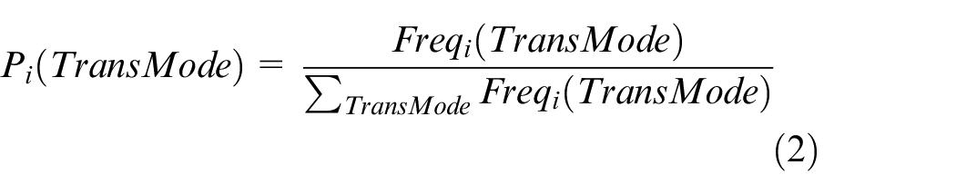
where P_i(TransMode) is the probability of transportation mode TransMode at grid index i. Freq_i (TransMode) is the frequency of GPS points of a specific transportation mode at grid index i. The denominator in equation (2) represents the total number of GPS points for all the transportation modes at grid index i.

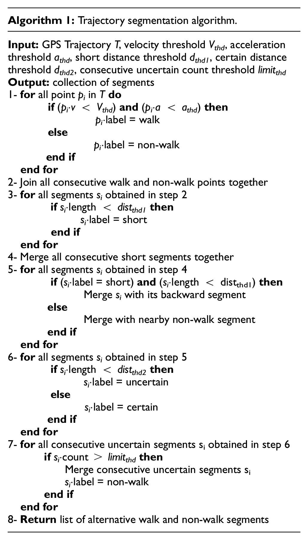
Segmentation

During the segmentation process, we will explain the procedure for the identification of change points in a GPS trajectory that results in candidate change points and the segments. We propose an enhanced segmentation algorithm for the identification of change points based on Zheng et al. ¹¹ and Zhu et al. ²⁰ and to further identify single-mode segments. The Zheng et al. ¹¹ method is created on the common-sense real-world knowledge that people first stop and then walk for some time to change their transportation mode, so walk is usually a transition between different transportation modes in most cases.

Our segmentation approach is different in the following way. As the velocities and acceleration of walk segments are usually consistent, it even behaves the same in congested traffic environment. However, it is possible that many walk points may appear in non-walk segments in congested traffic environment. Based on this fact, we design our algorithm as follows. First, all walk points and non-walk points are identified based on velocity and acceleration threshold values. Next, the sequence of walk and non-walk points is linked together to form a sequence of segments. If segment length is less than a particular threshold, it is considered as short segment; otherwise, it is considered as confirmed walk or non-walk segment as shown in Figure 3(a). Then, all consecutive short segments are combined together. In next step, if the length of short segment is still less than a particular threshold value, it will be merged with its backward walk or non-walk segment; otherwise, it is labeled as one non-walk segment, as shown in Figure 3(b). We only merge the shorter noisy segment with its backward segment that is less than a pre-defined length threshold, because only few noisy points in a segment usually do not affect the classification performance much. However, when a big noisy segment is merged with the other segment, it may affect the classification performance, because extracted features from big noisy segment dominate over the features of shorter length segment. Two non-walk points are identified in between the two walk segments as shown in Figure 3(b), so we merge these points with its backward segment based on the criteria of distance threshold dist_thd1. Then, user changes his transportation mode, and in the start of next segment, mixed mode of points are recorded due to traffic congestion or noise in the data that results in a sequence of shorter segments. So, we do not merge them one by one with the backward segment; instead, we treat such a sequence of shorter segments as one independent segment. As these segments have very high probability to be non-walk segment, we label them non-walk segment. In the next step, all consecutive walk and non-walk segments are connected together to form a sequence of walk and non-walk segments, as shown in Figure 3(c).

Figure 3.

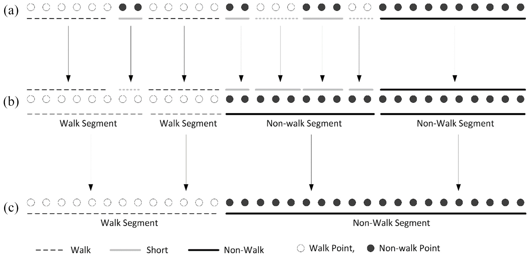
An example of segmentation.

It is generally believed that longer segments possess the richer features for the identification of transportation modes; such segments are considered as certain, while the shorter segments are highly uncertain. ⁷ Therefore, based on this fact, segments are further categorized either as uncertain or certain based on segment length threshold, that is, dist_thd2. At the end, we combine consecutive uncertain segments; if the sequence length of consecutive uncertain segments is greater than a threshold value limit_thd, we combine these uncertain segments and label them one non-walk segment. The detected change point is considered as correct if its distance from the ground truth lies in certain threshold range. Algorithm 1 describes the steps for the identification of change points and to segment the trajectories.

Algorithm 1: Trajectory segmentation algorithm.

Input: GPS Trajectory T, velocity threshold Vthd, acceleration threshold athd, short distance threshold dthd1, certain distance threshold dthd2, consecutive uncertain count threshold limitthd Output: collection of segments 1- for all point pi in T do    if (pi·v < Vthd) and (pi·a < athd) then      pi·label = walk    else       pi·label = non-walk   end if end for 2- Join all consecutive walk and non-walk points together 3- for all segments si obtained in step 2  ifsi·length < distthd1 then   si·label = short     end if end for 4- Merge all consecutive short segments together 5- for all segments si obtained in step 4  if (si·label = short) and (si·length < distthd1) then   Merge si with its backward segment  else    Merge with nearby non-walk segment  end if end for 6- for all segments si obtained in step 5  ifsi·length < distthd2 then   si·label = uncertain  else       si·label = certain  end if end for 7- for all consecutive uncertain segments si obtained in step 6  ifsi·count > limitthd then   Merge consecutive uncertain segments si   si·label = non-walk  end if end for 8- Return list of alternative walk and non-walk segments

Feature extraction

Feature extraction process provides the basis for classification models. Feature extraction is the process of creating features using domain knowledge, making machine learning methods work well. Thus, it is able to identify the transportation modes based on the feature vector obtained through feature engineering process. Inspired by relevant research, we extract 37 features in total, out of which 30 are borrowed from previous studies and 7 are newly proposed features as described in Table 1.

Table 1.

Features—summary table.

Studies	Features
Zheng et al. 11	Delta T, Expectation of Velocity, Mean Velocity, Mean Acceleration, Covariance of Velocity and Acceleration
Zheng et al. 16	Heading Change Rate, Stop Rate, Velocity Change Rate, Variance of Velocity, Max. Velocity, Max. Acceleration
Dabiri and Heaslip 3	Vincenty Distance, Bearing, Bearing Rate, Velocity, Acceleration, Jerk
Xiao et al. 14	25th and 75th percentiles of velocity and acceleration (25th V, 75th V, 25th A, 75th A), Interquartile Range of Velocity and Acceleration
Liang et al. 18	Velocity Rate (High/Medium/Low), Acceleration Rate (High/Medium/Low)
Zhu et al. 20	Time slice Type, Acceleration Change Rate, 85th V, 85th A, Max V2, Max A2, Median V, Median A, Expectation of Acceleration, Covariance V, Covariance A, Min V, Min A
Our new Features	Weekday, 4 × Transportation modes probabilities, Interquartile Mean of Velocity and Acceleration

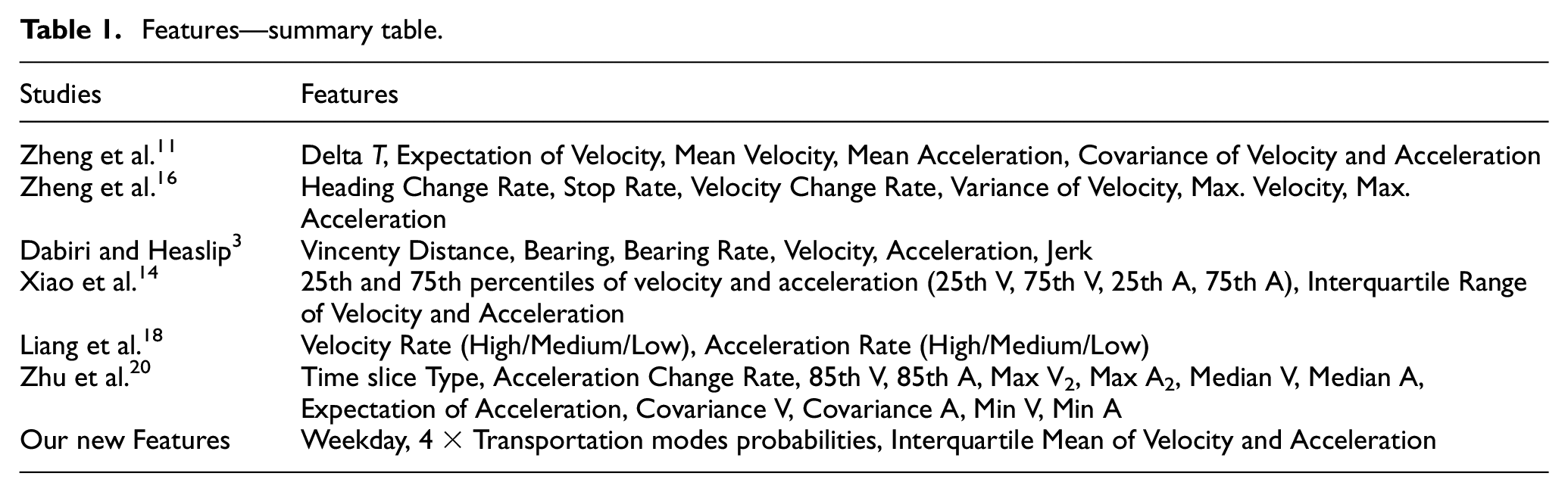
We identified the new set of features that are tolerant to traffic conditions in contrast to features used in previous studies. We combine all features in Table 1 to form a feature vector to feed into a classification model, which are more discriminative to identify transportation modes. Following is the description of our newly proposed features.

Weekday

When considering the transportation mode and the real-life behavior of the user, the patterns of transportation modes for the user may vary on working days and holidays. This is the category feature that tells the day of week is either a working day or weekend.

Interquartile mean

The motion features are sensitive to traffic conditions, so the statistical characteristics may not be useful to identify the transportation modes. For example, it is difficult to differentiate between the transportation modes based on its average velocities and acceleration values, because in traffic congestion the mean values of walk segment may be equal to car segment. The mean of interquartile values can differentiate between different transportation modes, so we introduce interquartile mean to avoid very low and very high outlier values of the segments.

Transport mode probability:

Four new features are identified from GPS data, one for each transportation mode, that is, the probability of transportation mode for a given segment. These probability distributions are averaged over all the grid cells (represented by grid indexes) from where the segments passed through. Then, these averaged probabilities for each transportation mode are used as the segment features, as given in equation (4)

$$P\left(\mathrm{TransMode}\right)=\frac{\sum _{\mathrm{for}\mathrm{all}inm}{P}_i\left(\mathrm{TransMode}\right)}{N}$$

(4)

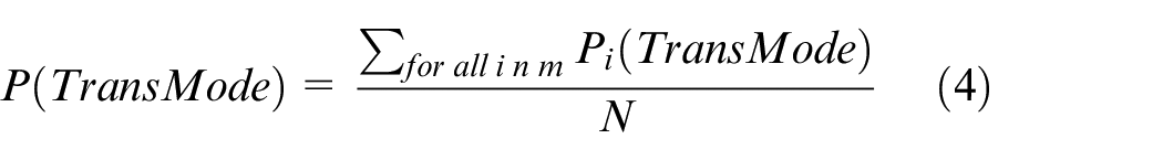
P(TransMode) is the probability of transportation mode TransMode for a segment, where m is the set of grid cells or grid indexes from which the segment passes through, N is the total number of grid cell indices from where the segment passed through. As shown in Figure 3, a segment passed through five different grid cells, and the segment probability of a given transportation mode is the average of probabilities for these five grid cells. As these grid cells are dominated by bus points, so the segment passed through these regions has high probability of being bus transportation mode.

Inference model

kNN and SVM are commonly used for classification tasks. However, previous studies^16,18,20 showed that tree-based algorithms performed better to identify the modes of transports. Therefore, on the basis of existing studies, we also used two traditional classifiers SVM and kNN. We selected three different tree-based classifiers including DT, Random Forest (RF) and Gradient Boosting Decision Tree (GBDT) to evaluate the performance of our methodology. The performances of these classifiers are compared for all kinds of transportation modes in our study including walk, bike, bus and car.

The input to the classification model is in the form (X, Y) = (x₁, x₂, x₃, …, x_k, Y), where X is a vector composed of features x₁, x₂, x₃ and so on, used for classification task and Y is our objective function, that is, to classify the mode of transport based on features vector X. Following is the brief description of classification models that we used in our experiments.

kNN

kNN is a proximity algorithm, the simplest and widely used algorithm, in which each data point is represented by its k neighbors and assigned the class with majority votes.

SVM

SVM ⁴⁴ is a widely used classification algorithm that separates the high dimensional data space into multiple classes through hyperplanes. Each hyperplane acts as a boundary between two distinct classes. The best hyperplane is the one having maximum distance to the nearest data points of neighboring classes.

DT

DT is widely used and powerful classifier that works on the principle of recursive partitioning. Recursive partitioning splits the tree into multiple subtrees based on independent variables for classification purpose. The process of splitting stops when it no longer increases value to prediction. DT also provides foundation for ensemble methods such as RF and bagging. DT sometimes overfits the data and suffers from high variance.

RF

RF ⁴⁵ is an ensemble classifier that trains the model by averaging the number of deep DT to predict the output class. RF overcomes the problem of overfitting in DT by reducing the variance, but with the cost of increase in bias. However, the final model greatly improves the performance.

GBDT

GBDT ⁴⁶ is a boosting method and also uses ensemble of multiple trees, as the RF does. It builds on the series of weak learner classifiers, where each classifier is trained to rectify the errors made by previous classifier in a series. Weak learners are shallow DT. It reduces error by reducing bias, but with little increase in variance. GBDT gives better performance than RF in most cases, but RF has the capability to train all classifiers in parallel, while GBDT trains these classifiers in sequence, as the input of next classifier is dependent on the output of previous classifier in a series.

Experiments

In this section, we demonstrate the experimental results to evaluate our framework. We will first describe the GPS data used for our experiments. Next, we will describe the selection of parameters. Finally, the results of detailed experiments will be explained. For all these experiments, we used Python version 3.7 with Scikit learn library version 0.20.0. For the analysis of geographical data, we used ArcMap v.10.3.

GPS data model

Our study is based on the Microsoft GeoLife data set, and part of the data set is visualized in Figure 4. The data set is collected by the 182 users in the GeoLife project version 1.3 over a 5-year period from April 2007 to August 2012.^16,47,48 More than 90% of the GPS trajectories were logged in dense representation with the sampling rate of 1–5 s or in a distance of 5–10 m between two consecutive points. This variation in the sampling rate between 1 and 5 s or between 5 and 10 m does not affect the classification performance, because the users do not change their directions frequently in such a short duration and distance. However, in very few occasions, the behavioral features like the heading change may not be calculated precisely, but this loss in precision does not affect the classification performance of transportation modes. The data set is created for over 30 cities of China and most of this recorded in Beijing that has the complex road and transportation network. Out of the total 182 users, 73 of them have labeled their trajectories with transportation modes including walk, car, bus, bike and train.

Figure 4.

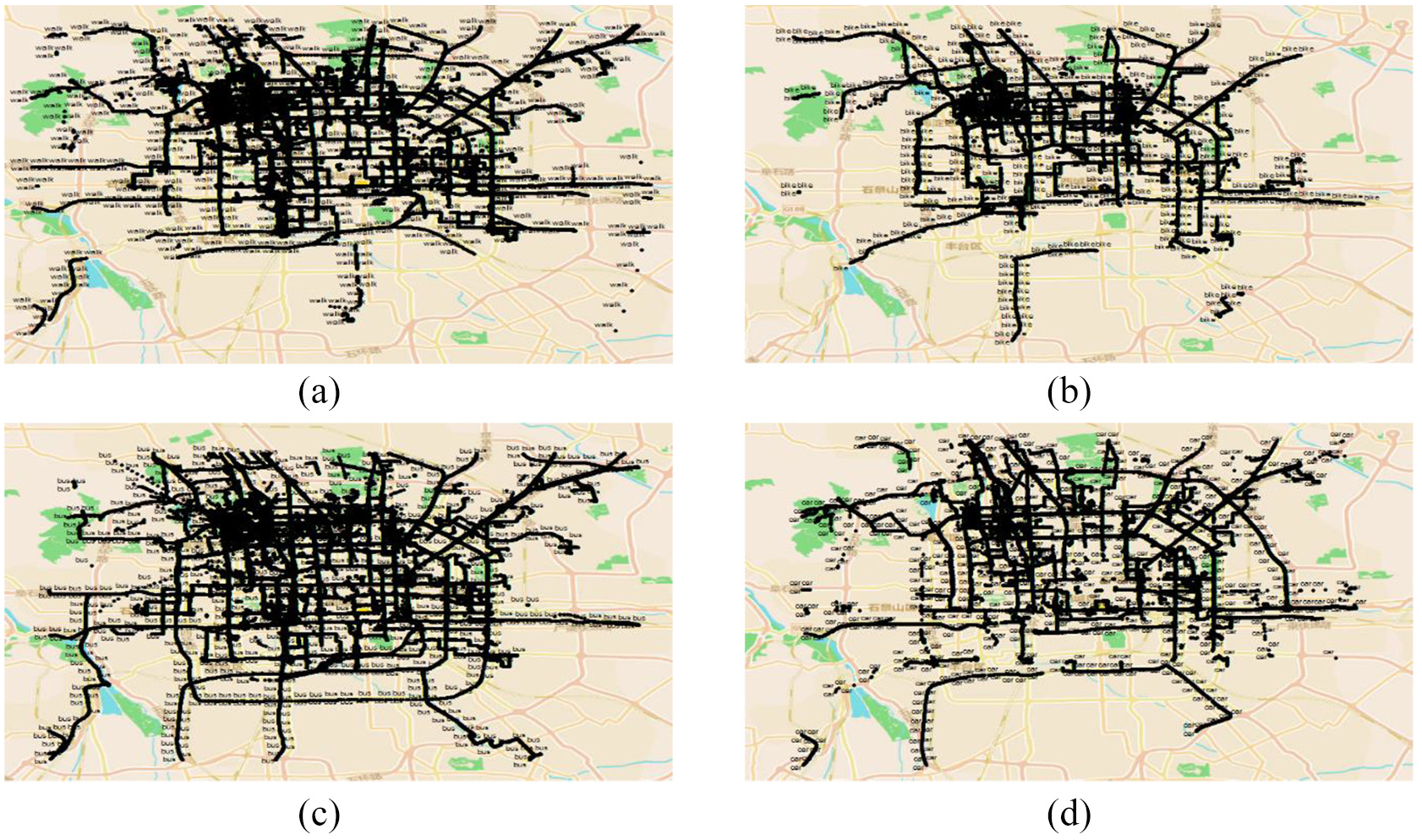
Microsoft GeoLife data set for Beijing: (a) walk, (b) bike, (c) bus and (d) car.

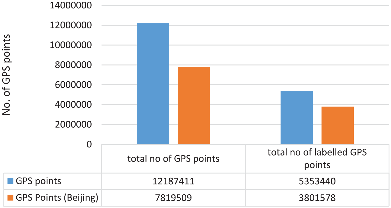
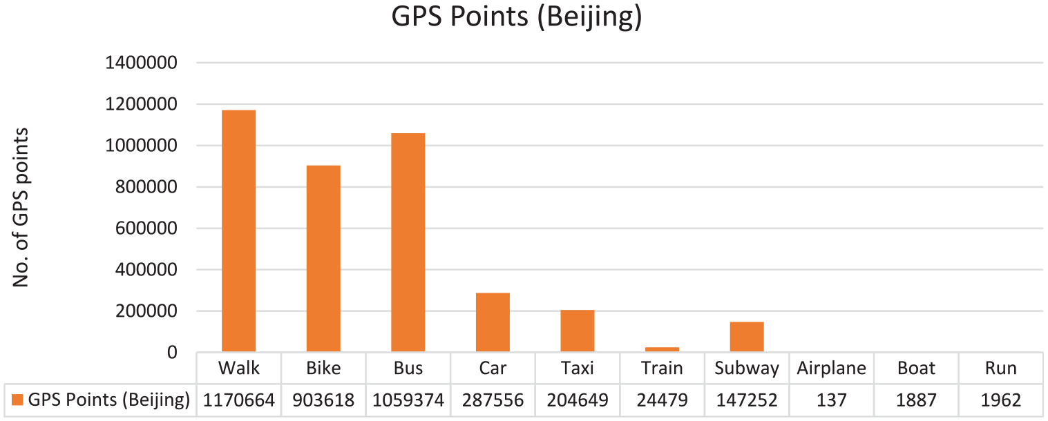
The data set of GeoLife project ¹⁶ is distributed over almost 30 cities of China, having almost 30,000 km of distance. The data set has 12,187,411 GPS points in total; out of them, 5,353,440 points are labeled. A total of 70% of the labeled points are recorded in Beijing city as shown in Figure 5. The representation of data is also dense in Beijing as shown in Figure 4, so we only consider the data for Beijing city in our experiments. Figure 6 shows the distribution of different transportation modes inside Beijing. As there is not enough data available for all the transportation modes inside Beijing, we only consider top 5 transportation modes having more than 200 thousand points as shown in Figure 6. Although subway has enough data available, but due to its low sampling rate, we do not consider subway mode in our experiments. Due to the similarity in the behavior of car and taxi, we treat all the taxi points as the car points. Therefore, our final list of transportation modes contains walk, bike, bus and car.

Figure 5.

GPS points distribution graph.

Figure 6.

GPS points distribution with their transportation modes.

After data preprocessing, 6927 single-mode segments are extracted from user trajectories; 70% of the data set is used to train the model and the remaining 30% is used as test data. Table 2 shows the distribution of segments with respect to their transportation modes.

Table 2.

The distribution of different transportation modes.

Transportationmodes	Number ofsegments	Distance (km)	Time (h)
Walk	2617	9137	10,629
Bike	1327	5686	8379
Bus	2047	10919	8665
Car	936	8907	5449

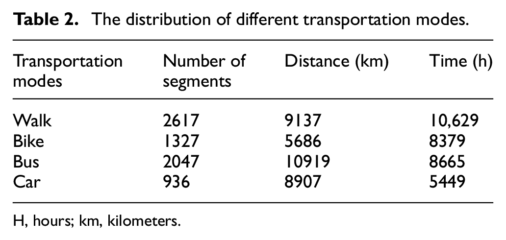
H, hours; km, kilometers.

Parameters

In the preprocessing step, the label files are joined with the GPS track file for each user to make full tracks for all users. Tracks are partitioned into trips, if the difference of timestamps between two consecutive points is greater than 20-min interval threshold. When using Algorithm 1 to label the points, the values for velocity and acceleration threshold V_thd, a_thd are 1.8 m/s and 0.6 m/s², respectively. ¹¹ Threshold value for consecutive uncertain segment limit_thd is set to 3 in segmentation algorithms. We set the distance threshold dist_thd1 = 10 m and dist_thd2 = 50 m for Algorithm 1, where we get the maximum precision with acceptable recall for the identification of change points. Threshold values for the features Heading Change Rate (HCR), Stop Rate (SR) and Velocity Change Rate (VCR) equal 19, 3.4 and 0.26, respectively. ¹⁶ Weekday features store two types of possible values 0 and 1; 1 means working days from Monday to Friday, and 0 means weekend representing Saturday and Sunday. In our problem, recall is more important than precision, because we want to retrieve as many as possible from all ground truth change points. ¹¹ The predicted change points are considered correctly identified, if ground truth change point exists within the distance of 150 m from identified change point. ¹¹ We divide the geographical space of Beijing into 2D cell grids with 72 columns and 60 rows, where each grid cell is of size 500 m².

Evaluation

To validate the effectiveness of our approach, we use different evaluation metrics including precision, recall, F score and accuracy. Performance of segmentation algorithm and new features are evaluated using precision, recall and F score. The accuracies of our method and existing methods are compared at the end of this section.

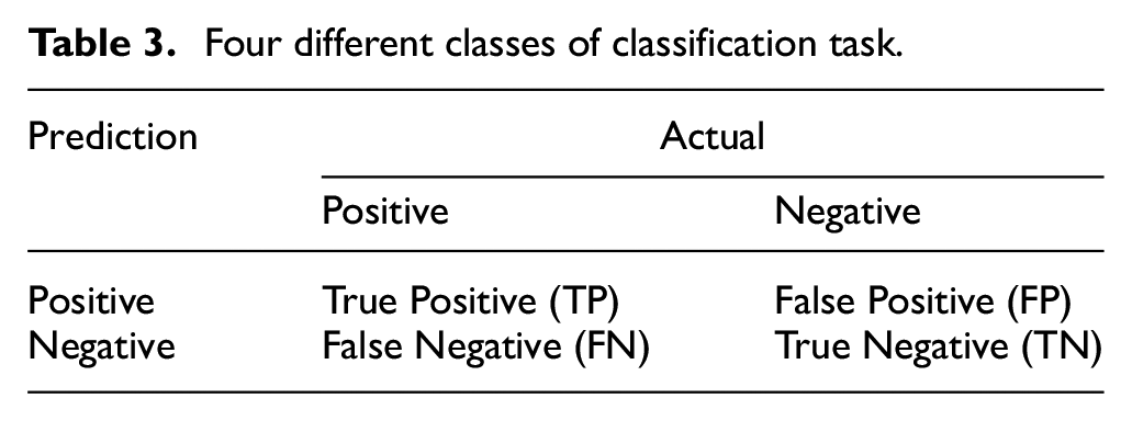
We briefly introduce the evaluation metrics. We divide our classification task into four different classes, as shown in Table 3:

• True Positive (TP). Actual instances that are true and also predicted true.

• False Positive (FP). Actual instances that are true but predicted false.

• True Negative (TN). Actual instances that are false and also predicted false.

• False Negative (FN). Actual instances that are false but predicted true.

Table 3.

Four different classes of classification task.

Prediction	Actual
	Positive	Negative
Positive	True Positive (TP)	False Positive (FP)
Negative	False Negative (FN)	True Negative (TN)

Precision is the fraction of all correctly identified instances out of all identified instances. The mathematical form of precision is given in equation (5)

$$\mathrm{Precision}=\frac{\mathrm{TP}}{\mathrm{TP}+\mathrm{FP}}$$

(5)

Recall is the fraction of all correctly identified instances out of all the instances that should be classified correct. Equation (6) is the mathematical form of recall

$$\mathrm{Recall}=\frac{\mathrm{TP}}{\mathrm{TP}+\mathrm{FN}}$$

(6)

F score is the harmonic mean of precision and recall and calculated using equation (7) given below

$$F\mathrm{score}=\frac{2\times \mathrm{Precision}\times \mathrm{Recall}}{\mathrm{Precision}+\mathrm{Recall}}$$

(7)

Accuracy is the ratio of all the instances correctly classified to the total number of all the instances. Mathematical form of accuracy is given in equation (8)

$$\mathrm{Accuracy}=\frac{\mathrm{TP}+\mathrm{TN}}{\mathrm{TP}+\mathrm{FP}+\mathrm{TN}+\mathrm{FN}}$$

(8)

Evaluation on segmentation

We considered four baseline segmentation methods including Fixed Length Segment (FLS), Fixed Duration Segment (FDS) and the method of Liang et al. ¹⁸ and Zheng et al. ¹¹ to compare the performance of our segmentation method. Table 4 shows the comparison of above-mentioned segmentation methods with our method in terms of precision and recall. Recall is more important than precision to retrieve maximum possible ground truth change points; however, precision of change points is also important to retrieve as many as small number of larger segments. ¹¹ If all points of GPS trajectory are retrieved as change points, it will give 100% recall, and all the segments contain only one GPS point that does not give meaningful information about the segment for prediction. Our segmentation method outperforms the benchmark methods, in all aspects of precision, recall and F score, as shown in Table 4.

Table 4.

Comparison of different segmentation methods of GPS trajectories.

Measure (%)	Methods
	FLS	FDS	Liang et al.	Zheng et al.	MoISP
Precision	16.31	21.44	42.73	39.98	43.36
Recall	81.15	84.82	85.93	86.31	88.17
F1 score	27.16	34.22	57.07	54.64	58.13

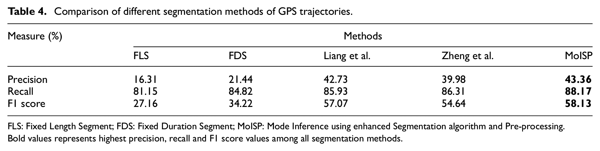
FLS: Fixed Length Segment; FDS: Fixed Duration Segment; MoISP: Mode Inference using enhanced Segmentation algorithm and Pre-processing.

Bold values represents highest precision, recall and F1 score values among all segmentation methods.

Feature evaluation

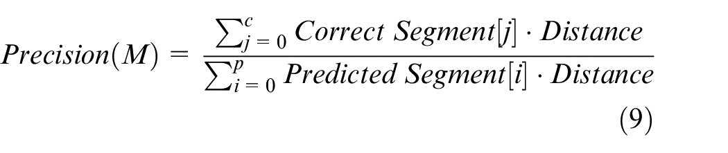
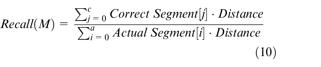
Performance evaluation of new proposed features in order to classify modes of transport: we compare its effectiveness with the existing features in this section. We choose RF as our classification model for the purpose of feature evaluation. Table 5 presents the comparison of precision, recall and F score of different set of features for all transportation modes. It also presents the overall accuracy on different set of features. We focus on the accuracy by distance (A_D), which is the accuracy of the distance covered by different transportation modes, which is more objective than the accuracy by number of segments. ¹¹ Precision is the fraction of distance covered by correctly identified instances and the distance covered by the total number of classified instances of mode M, whereas Recall is correctly identified instances out of the actual instances. The precision and recall are given in equations (9) and (10)

$$\mathrm{Precision}\left(M\right)=\frac{\sum _{j=0}^c\mathrm{Correct}\mathrm{Segment}\left[j\right]·\mathrm{Distance}}{\sum _{i=0}^p\mathrm{Predicted}\mathrm{Segment}\left[i\right]·\mathrm{Distance}}$$

(9)

$$\mathrm{Recall}\left(M\right)=\frac{\sum _{j=0}^c\mathrm{Correct}\mathrm{Segment}\left[j\right]·\mathrm{Distance}}{\sum _{i=0}^a\mathrm{Actual}\mathrm{Segment}\left[i\right]·\mathrm{Distance}}$$

(10)

Table 5.

Feature comparison.

Mode	New features (%)			Existing features (%)			Combined features (%)
	Precision	Recall	F score	Precision	Recall	F score	Precision	Recall	F score
Walk	59.53	66.69	62.91	94.97	96.03	95.5	95	97.39	96.18
Bike	49.33	52	50.63	89.15	90.04	89.59	92.1	93.07	92.59
Bus	63.61	57.14	60.20	95.46	87.35	91.23	95.06	92.40	93.71
Car	65.71	66.76	66.23	85.51	95.03	90.02	92.89	94.19	93.53
Accuracy (%)	60.65			91.52			93.99

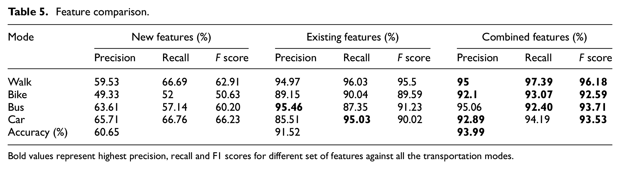
Bold values represent highest precision, recall and F1 scores for different set of features against all the transportation modes.

where c is correctly identified segments of transportation mode M, p is the total number of predicted segments of mode M and a is the actual number of segments of transportation mode M.

The accuracy of the segments is the fraction of distance covered by all correctly classified segments, out of the total distance of all the segments, as given in equation (11)

$$A_D=\frac{\sum _{j=0}^m\mathrm{Correct}\mathrm{Segment}\left[j\right]·\mathrm{Distance}}{\sum _{i=0}^N\mathrm{Segment}\left[i\right]·\mathrm{Distance}}$$

(11)

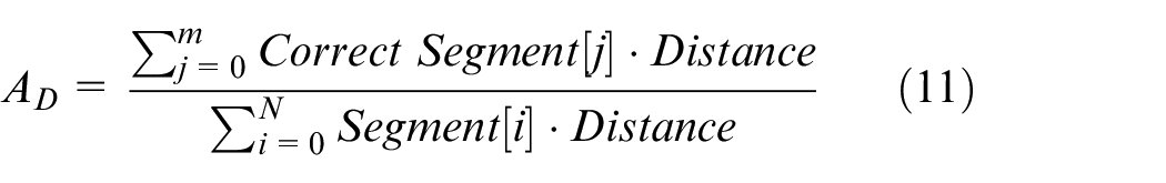
A_D is the accuracy of segments by distance, N denotes the total count of segments, whereas m stands for correctly classified segments.

We categorize the features into three sets. The first set contains the newly proposed features only, the second set contains the existing features and the third is the combined set of features, which is combination of newly proposed features and existing feature set. We evaluate the performance on all three sets of features using RF algorithm, based on different performance measure criteria mentioned in equations (7), (9) and (10). The results of Table 5 show that our newly proposed features (when used alone) can correctly identify almost 60% of the distances of all transportation modes. The precision of bus is slightly less with combined features, but there is enormous increase in the recall; similarly, recall of car mode is slightly less as compared to existing features, but combined features achieved better precision for car mode. When new features are combined with existing features, there is significant improvement in terms of both F score and accuracy for all the transportation modes.

Model evaluation

We perform the evaluation of our methodology using five different classifiers: kNN, SVM, DT, RF and GBDT. We trained all these classifiers using default parameters of Scikit learn, the python library for machine learning tasks. Tables 6–10 present the results of these classifiers in terms of precision, recall and accuracies for all the transportation modes.

Table 6.

Confusion matrix of kNN.

kNN		Actual (%)				Precision (%)
		Walk	Bike	Bus	Car
Predict (%)	Walk	84.81	8.14	3.15	2.46	84.71
	Bike	13.32	74.58	7.33	1.98	67.77
	Bus	1.86	12.98	80.69	15.64	82.32
	Car	0	4.28	8.81	79.90	83.19
Recall (%)		84.81	74.58	80.69	79.90	80.31

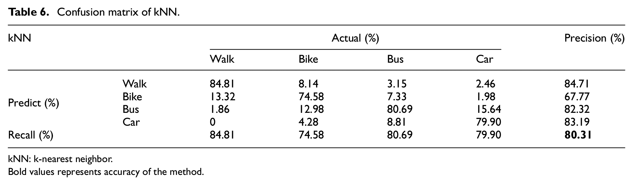
kNN: k-nearest neighbor.

Bold values represents accuracy of the method.

Table 7.

Confusion matrix of support vector machine.

SVM		Actual (%)				Precision (%)
		Walk	Bike	Bus	Car
Predict (%)	Walk	94.39	7.21	2.12	1.79	88.82
	Bike	5.30	85.86	5.90	1.79	79.44
	Bus	0.29	5.18	85.14	8.17	91.45
	Car	0	1.74	6.82	88.23	88.52
Recall (%)		94.39	85.86	85.14	88.23	87.95

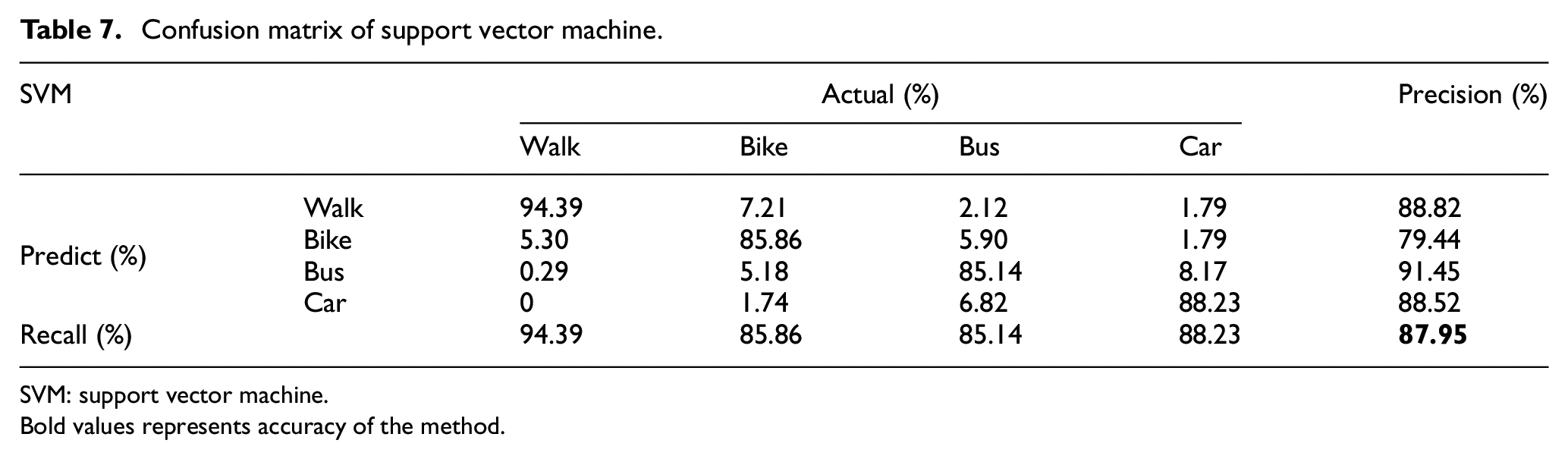
SVM: support vector machine.

Bold values represents accuracy of the method.

Table 8.

Confusion matrix of decision tree.

Decision Tree		Actual (%)				Precision (%)
		Walk	Bike	Bus	Car
Predict (%)	Walk	93.29	2.90	0.73	0.36	95.74
	Bike	3.72	85.29	1.89	1.46	88.64
	Bus	2.31	9.53	89.41	9.19	88.40
	Car	0.66	2.26	7.95	88.96	86.37
Recall (%)		93.29	85.29	89.41	88.96	89.40

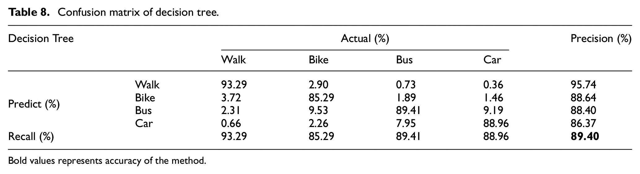
Bold values represents accuracy of the method.

Table 9.

Confusion matrix of random forest.

Random Forest		Actual (%)				Precision (%)
		Walk	Bike	Bus	Car
Predict (%)	Walk	97.39	3.10	1.06	0.54	95.00
	Bike	1.54	93.07	2.24	0.75	92.10
	Bus	0.99	2.74	92.40	4.50	95.06
	Car	0.06	1.07	4.27	94.19	92.89
Recall (%)		97.39	93.07	92.40	94.19	93.99

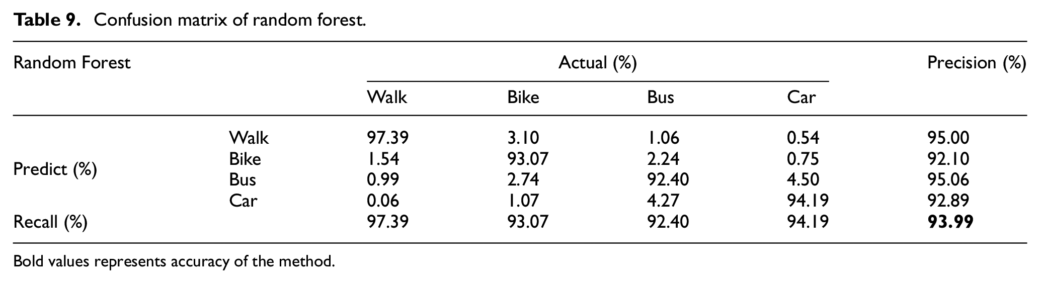
Bold values represents accuracy of the method.

Table 10.

Confusion matrix of GBDT.

GBDT		Actual (%)				Precision (%)
		Walk	Bike	Bus	Car
Predict (%)	Walk	99.27	6.22	1.71	0.61	91.75
	Bike	0.19	92.89	2.67	2.23	90.77
	Bus	0	0.88	89.52	16.14	88.92
	Car	0.53	0	6.07	81.00	89.43
Recall (%)		99.27	92.89	89.52	81.00	89.99

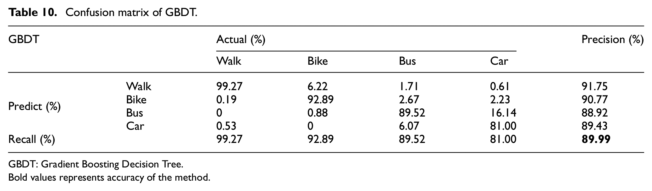
GBDT: Gradient Boosting Decision Tree.

Bold values represents accuracy of the method.

The end value in bold font of Table 6 is the overall accuracy of kNN classifier for all transportation modes.

The SVM model performs better than kNN classifier, in terms of precision, recall and accuracies of all transportation modes. Tables 6 and 7 show the results of kNN and SVM classifier.

While comparing RF with DT classifier shown in Tables 8 and 9, it can be seen that precision of walk transportation mode is slightly better than RF; however, there is significant increase in precision for all other transportation modes in case of RF, and recall of RF is too better than DT for all transportation modes. There is 4.5% increase in overall accuracy of RF classifier.

The overall accuracy of GBDT as shown in Table 10 is slightly better than DT, but too less than RF. RF classifier outperforms all the classifiers that we use to evaluate our methodology. DT has better precision of walk mode than RF, and GBDT has better recall of walk mode than RF. However, in all other aspects, RF outperforms DT and GBDT in our methodology.

Table 11 and Figure 7 show the accuracies of five classifiers: kNN, SVM, DT, GBDT and RF. Accuracy of GBDT is better than RF in walk mode, but for all other transportation modes, RF achieved better accuracy as compared to all other models. RF classifier also outperforms in overall accuracy for all the transportation modes.

Table 11.

Accuracy comparison for all transportation modes.

Models	Walk (%)	Bike (%)	Bus (%)	Car (%)	All (%)
kNN	84.81	74.58	80.69	79.9	80.31
SVM	94.39	85.86	85.14	88.23	87.95
DT	93.29	85.29	89.41	88.96	89.4
GBDT	99.27	92.89	89.52	81	89.99
RF	97.39	93.07	92.4	94.19	93.99

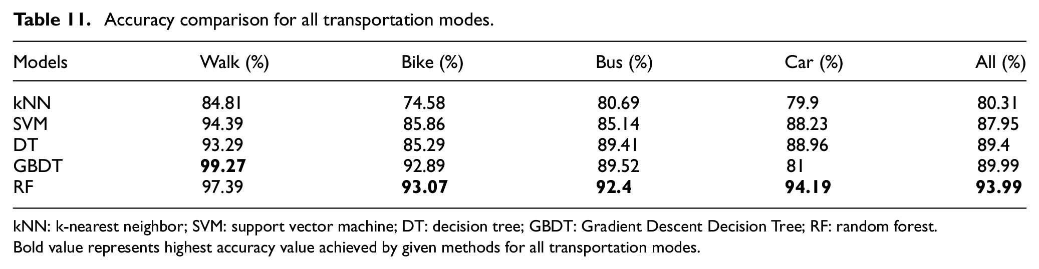
kNN: k-nearest neighbor; SVM: support vector machine; DT: decision tree; GBDT: Gradient Descent Decision Tree; RF: random forest.

Bold value represents highest accuracy value achieved by given methods for all transportation modes.

Figure 7.

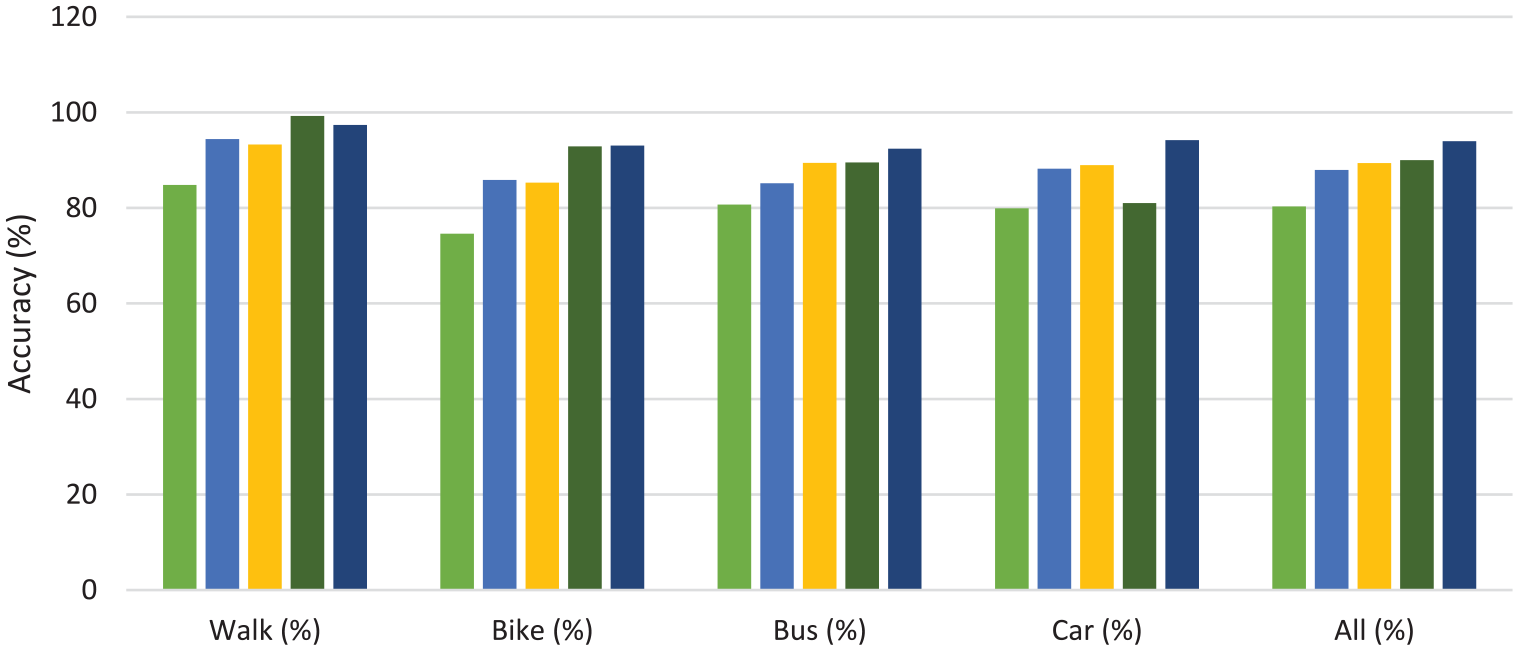
Comparison of classifiers for all transportation modes.

Comparison of transportation mode methods

To evaluate the effectiveness of our study for identifying the transportation modes, we compare our method (MoISP) with the existing studies using the same GeoLife data set in their experiment. To make the comparison, we considered three relevant studies including some previous studies^3,16,18,20 for comparison with our method. Table 12 presents the accuracy results of these studies and our method, which show the best accuracy of our method as compared to all other methods. More transportation modes can be identified using our approach provided the sufficient availability of data for each transportation mode.

Table 12.

Comparison of transportation modes.

Study	Accuracy
Zheng et al. 16	86.21
Liang et al. 18	89.24
Zhu et al. 20	82.81
Dabiri et al. 3	85.73
MoISP	93.99

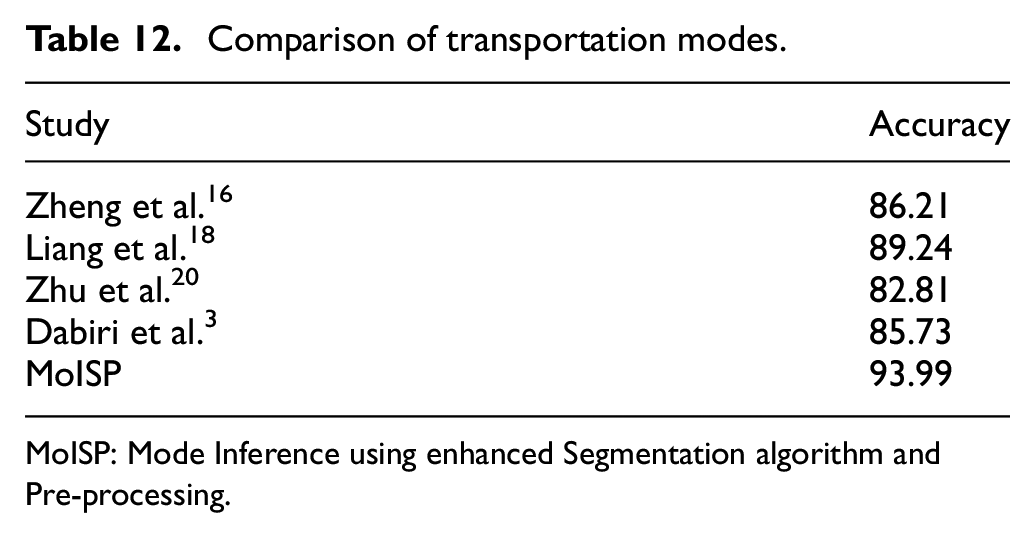
MoISP: Mode Inference using enhanced Segmentation algorithm and Pre-processing.

Conclusion

We proposed the framework MoISP for the classification of four types of transportation modes including walk, bike, bus and car, using our proposed framework. Our framework comprises of new preprocessing technique, segmentation algorithm and the identification of new features from raw GPS trajectory data that are more robust even in a complex city network. The reason for considering only four transportation modes is the lack of availability of data for all transportation modes. In data preprocessing stage, anomalous data are removed from trajectories, point-level features are extracted and probability distribution function is calculated for geospatial regions. We proposed a segmentation approach to partition the user’s trajectories into multiple single-mode segments that achieves best precision and recall values for change points in comparison with existing studies. Our newly proposed features make the significant improvement in precision and recall values for almost all the transportation modes. Our study of inferring transportation modes also achieves best accuracy results in comparison with benchmark methods. The advantage of our approach is that it only uses GPS data to identify new spatial features, in addition to the existing motion-based features that affect the classification performance in abnormal traffic conditions.