
Abstract
The paper reports an adaptive-network-based fuzzy inference system for the measurement of axial strain using long-period fiber grating sensors. The long-period fiber grating sensor supports optical resonances, which are sensitive to the change of axial strain. The axial strain can be quantified based on the wavelength shift and amplitude changes of the optical resonance. To improve the accuracy of axial strain quantification, this paper proposes the adaptive-network-based fuzzy inference system model. The adaptive-network-based fuzzy inference system model is trained using the strain data measured with long-period fiber grating sensors. The parameters of the membership functions used in the adaptive-network-based fuzzy inference system are set adaptively. In the adaptive-network-based fuzzy inference system–based method, the maximum relative error was found to be 1.5%, which is about one-ninth of that when the data fitting method was used. The R-squared statistics using the adaptive-network-based fuzzy inference system model is 0.9872, while that using the linear fitting algorithm is 0.8815. Compared with the conventional data fitting methods, the proposed approach is highly adaptive and versatile with the capability of improving the accuracy of strain quantification.
Introduction
Since strain sensors can measure deformation and vibration responses of structures, they have been widely used for structural health monitoring to detect and evaluate system damages. There are different types of strain sensors, such as capacitive,1,2 inductive, 3 resistive, 4 and piezoelectric strain gauges.5,6 However, most of these strain sensors are based on electrical transducers, which have limitations in sensitivity, reliability, and accuracy. In addition, the electrical strain transducers are vulnerable to potential electromagnetic interferences. In contrast, optical strain sensors, such as the long-period fiber grating (LPFG) sensor, have attracted considerable attention in the engineering community. The LPFG sensor has the advantages of having a small size, low weight, anti-electromagnetic interference, high durability, and resistance to corrosion. LPFG sensors are sensitive to many environmental factors, such as temperature, 7 strain, 8 bending, 9 and refractive index.10,11
The working principle of a LPFG sensor is based on the shift of the resonance wavelength that occurs when the LPFG is subjected to external physical parameters such as strain. Therefore, the ability to determine the relationship between the external parameter and resonance wavelength with adequate accuracy is essential. Generally, the curve fitting algorithm can be used to improve the estimation accuracy. The common curve fitting algorithms include the centroid method, 12 general polynomial fitting, 13 genetic algorithm, 14 and Gaussian nonlinear fitting. 15 The first two methods are simple; however, the demodulation accuracy is low, and the anti-noise performance is poor. The last two algorithms have high accuracy; however, they depend on the initial value; therefore, a substantial amount of calculation is required at the early stage.
At present, polynomial fitting is widely used for data processing in LPFGs, some other schemes have been discussed in the literatures too. Combining active laser frequency sweeping with unwrapping algorithms, relationship between strain value and variation of interference power is set up. 16 Using the strain field measured on the specimen surface with electronic speckle pattern interferometry and a discretized model of the grating, the spectra in transmission are verified analytically. 17 By point-by-point direct writing technique, an overlapping of the first-order and second-order spectrum is then observed. 18 An improved phase-sensitive optical time-domain reflectometer (Φ-OTDR) system based on ultra-weak fiber Bragg grating (FBG) arrays is used to realize quantitative strain measurement using narrow pulse. 19 These new methods evolved from the traditional basic methods. Therefore, they include the disadvantages of the traditional schemes.
The LPFG is sensitive to several parameters. When the fiber grating is used for axial strain sensing, there may be cross sensitivity and interference. Theoretical study shows that the relationship between the LPFG’s wavelength and strain is nonlinear. But in practical application, it is often assumed that the relationship between them is linear, which will lead to some measurement errors.
In recent years, the use of artificial intelligence to interrogate optical sensors has acquired growing importance. Gill et al. 20 put forward a genetic algorithm for the interrogation of optical fibers Bragg grating strain sensors. At the same time, the transfer-matrix approach is used to replace the numerical solution of the coupled-mode equation. Lamberti et al. 21 presented a novel fast phase correlation detection algorithm, which computes the wavelength shift in the reflected spectrum of an FBG sensor. Ganziy et al. 22 suggested a novel dynamic gate algorithm for precise and accurate peak detection. The algorithm uses a threshold-determined detection window and the center of gravity algorithm with bias compensation. Srivastava and Kumar 23 determined the pH of solution employing an optical fiber sensor based on a sol–gel thin film and a multivariate calibration based on an artificial neural network (ANN).
The adaptive-network-based fuzzy inference system (ANFIS)24,25 model combines the advantages of fuzzy logic and neural networks with outstanding learning, approximation, and predictive capabilities. The ANFIS has been widely studied in the field of computer science. However, to the best of our knowledge, it has never been considered in LPFG strain applications so far. In this paper, an ANFIS model is proposed to boost the accuracy of LPFG strain sensors. We experimentally compared two data point fitting methods based on linear fitting algorithm and ANFIS, both implemented on spectra sensing by LPFG strain sensor. The calculated absolute error and R-squared statistics show that the ANFIS model can effectively improve the accuracy of strain quantification compared with the conventional data fitting method.
Principle of axial strain sensing using LPFG
The LPFG structure can be considered as an isotropic cylinder, whose strain can be affected by forces applied along all directions. Among the forces, the most practical one is the axial tension or compression force that produces the axial strain. Under an axial strain, the core and cladding materials are turned into anisotropic uniaxial crystals. As a result, the core and cladding modes along the fiber axis are changed. Pulling or squeezing the grating of LPFGs can lead to the change of the grating period. The core and cladding materials with photo elasticity also experience the changes of the refractive indices. Thus, under an axial strain, the resonance conditions of LPFGs are altered and thus the resonant signatures can change accordingly.
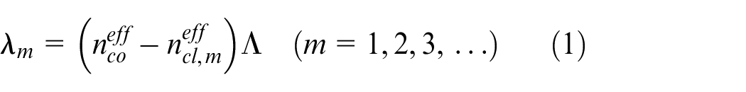
According to the coupled-mode theory,26–28 the phase matching condition of a LPFG is
where
where

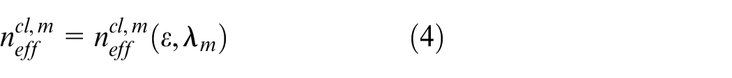
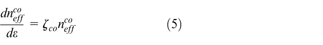
The effective refractive indices are given as
where
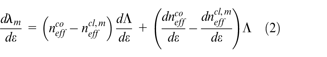
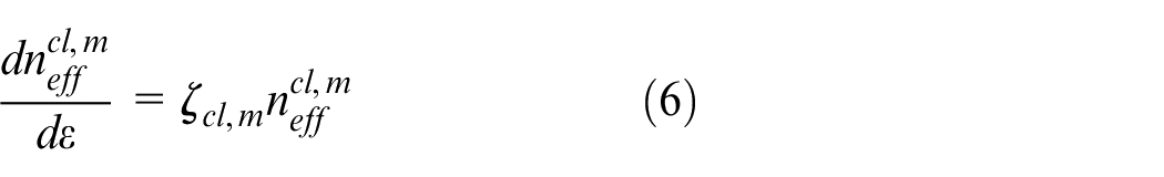
In equation (2), the first term represents the change of the refractive index of fiber or the propagation constant due to the elastic-optic effect induced by strain. The second term corresponds to the change of the grating period under an axial strain. It is also necessary to take the mode dispersion and material dispersion of optical fiber into consideration in the strain analysis. As it can be seen from equations (2)–(6), the axial strain sensitivity of LPFG is related to the materials of the optical fiber, the resonance wavelength determined by the grating period, and the order of the corresponding cladding mode.
ANFIS model
ANFIS combines neural network with fuzzy logic to construct nonlinear mapping model of input and output by introducing human experience and knowledge as the rules. An ANFIS model can update its own system parameters by the continuous learning of training data and generate an adaptive fuzzy inference system. The flow diagram of the ANFIS structure is shown in Figure 1. The connection among nodes only indicates the signal flow direction, and there is no weight associated with it. The square box represents the node with tunable parameters, and the circular node indicates that there is no tunable parameter. Among these five layers, only the first and fourth layers contain tunable parameters.
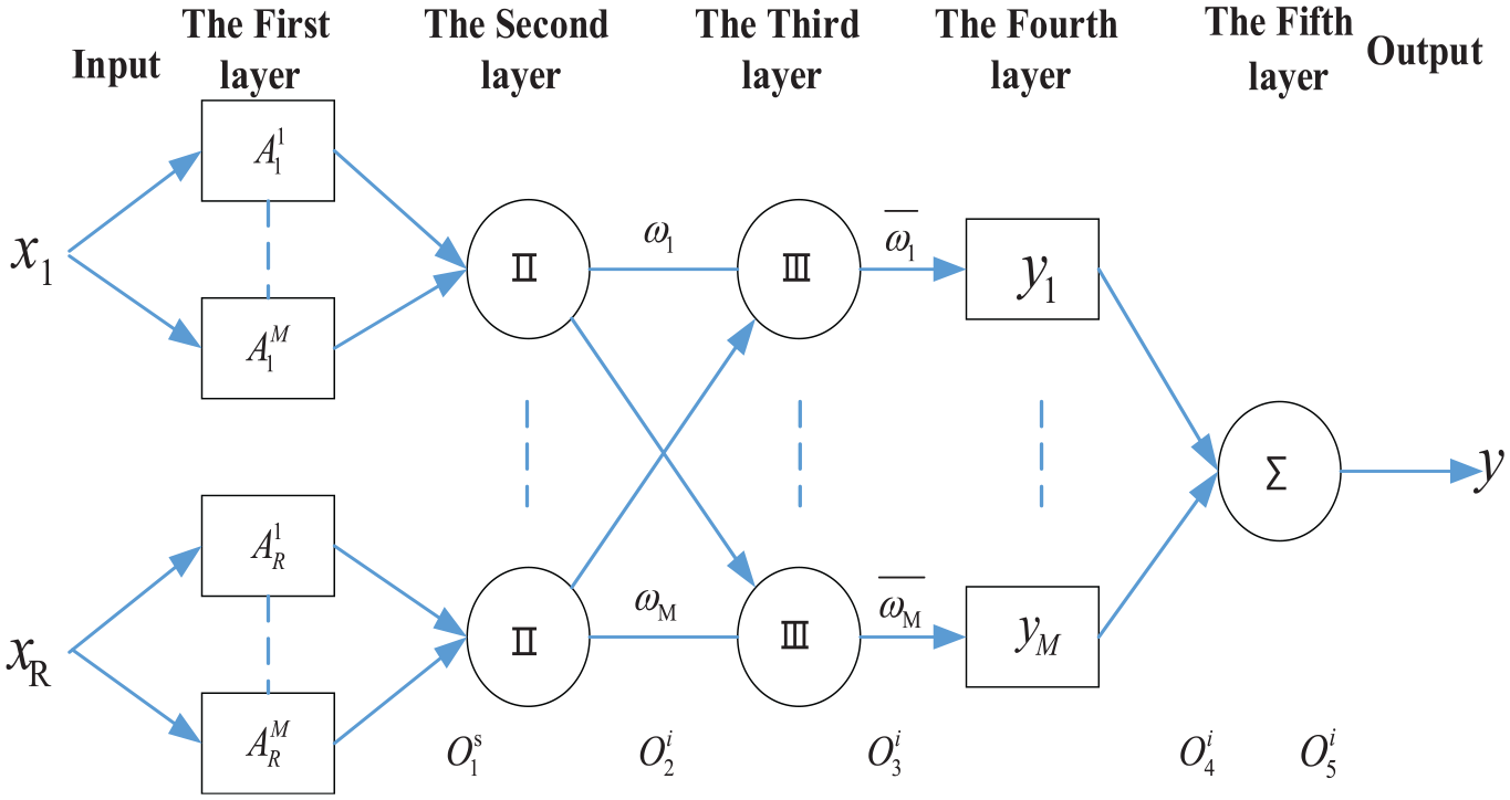
Flow chart of the ANFIS system.
The functions of each layer are as follows. The first layer is a fuzzification layer, where each node of the layer represents a linguistic variable value, the input variable is fuzzified, and the membership of the input variable to the fuzzy subset is obtained as
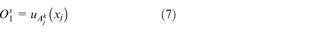
where
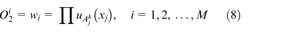
The second layer is the rule layer, which implements the operation of the fuzzy set of the premise. The output is the algebraic product of the input signals and indicates the activating strength of the sample to the rule. Each node of this layer represents a fuzzy rule used to match the fuzzy rule antecedent. The applicability of each fuzzy rule can be calculated by multiplicative reasoning as
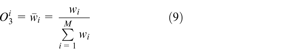
The third layer is the normalized layer, which normalizes the excitation strength of each rule as
The fourth layer is the adaptive output layer. Each node i of this layer is an adaptive node with a node function that computes the output of each rule as

where
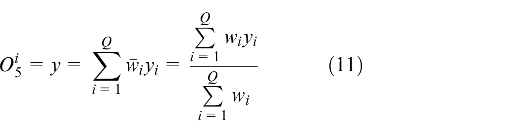
The fifth layer is the defuzzification layer, which implements a sharpening calculation to find the sum of the outputs of all rules as the total output given by
Construction of ANFIS model for axial strain quantification
Acquisition of experimental data
Figure 2 shows the experimental setup of the LPFG-based axial strain measurement. The LPFG sensor was fixed on the Mechanical Testing & Simulation(MTS) drawing mill, and tensile stresses were applied on the surface of the specimen by the mill. During the experiments, a broadband light (83437A, Agilent) was used as the excitation and an optical spectrum analyzer (AQ6317C, Yokogawa) was used to measure the transmission spectrum through the LPFG sensor with the spectral resolution of 0.02 nm. The grating length is 4 cm, and the central wavelength is 1530 nm. The axial strain measurements were carried out under a stabilized temperature at 25 °C. The influence of the temperature fluctuation on the LPFG sensor can be ignored.
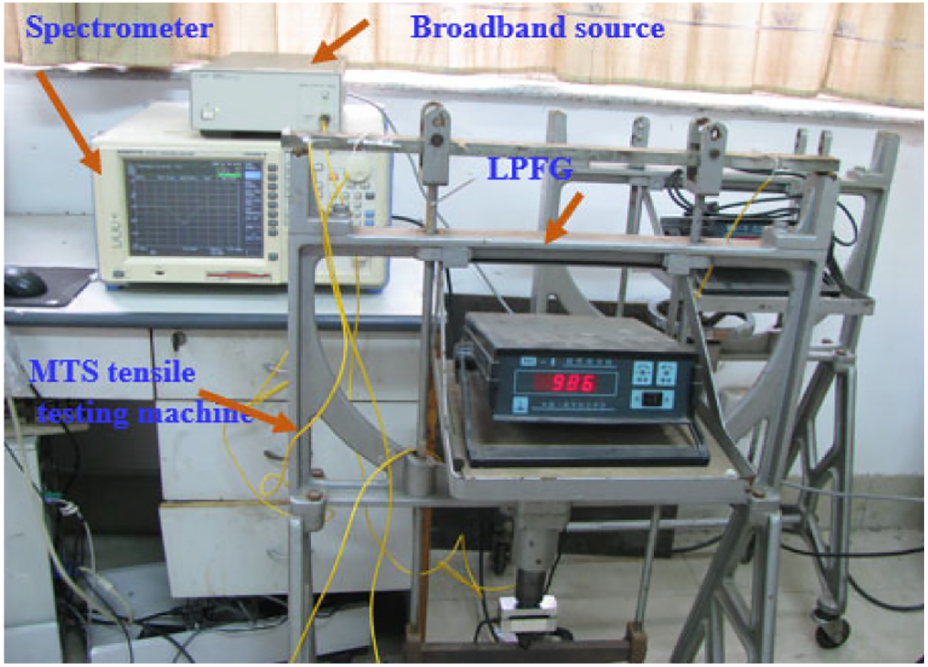
Axial strain measurement setup.
Figure 3 illustrates the tensile testing machine used for the force analysis. F is the stress generated by the tensile test machine. According to the principle of force balance, the support force, N, should be equal to F. The distance between point A and point P, which are arbitrary points lies between points B and C, is x. The bending moment can be calculated based on the material mechanics as

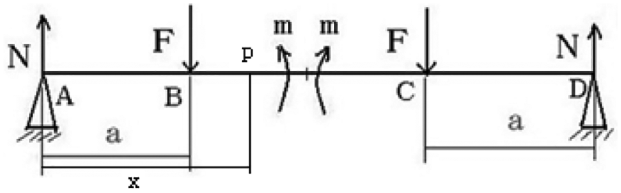
Force analysis of tensile test machine.
Any point between points B and C is subjected to the same bending moment. The stress F of dynamometer can read by a digital instrument, and the force applied at the points A and D is the bending moment between point B and C. As shown in Figure 4, the LPFG sensor was glued to the steel surface. Because the LPFG fiber is small compared to the measurement instrument, the stress applied on the lower surface of the steel is the same as the stress of the LPFG sensor. During the experiment, the axial stress was produced by the pressure applied to steel using the tensile test machine.
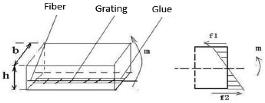
Schematic of the fixed LPFG under axial stress.
With the knowledge of material mechanics, the relationship among the stress (
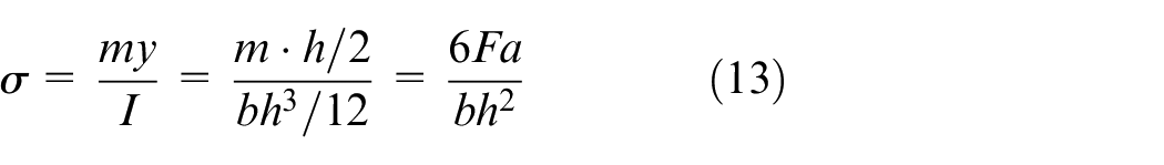
where
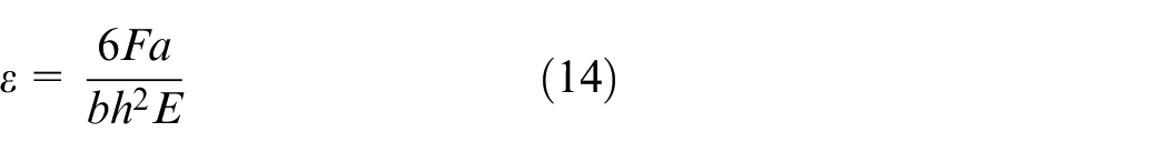
where E refers to the elastic modulus, which is 210 GPa for the 45 steel.
During the test, the tensile strains were applied to the LPFG sensor in the range of 0–3000 N with the increment of 100 N. The fourth-order resonant wavelength was adopted in this paper. Figure 5 shows the transmission spectra measured when the LPFG sensor was placed under the axial strains of 50, 200, 400 N, and so on.
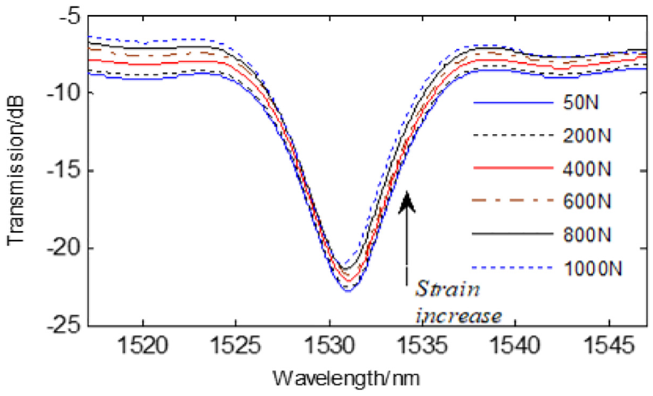
LPFG spectra vary with axial strain.
Determination of the ANFIS model
The ANFIS model was used to determinate the strains based on the measured transmission spectra. The input variables are the wavelength and amplitude of the LPFG resonance, and the output variable is the axial strain. The number of nodes in the first layer is the product of the number of fuzzy rules of each input variable. The number of input variables is 2, and the number of fuzzy rules is 10. Thus, the number of total nodes in the first layer is 20. The number of nodes in the second layer is the number of fuzzy rules, which is equal to 10. The numbers of nodes in the third and fourth layers are 10, which is the same as that in the second layer. The number of nodes in the fifth layer is equal to the number of output variables which is equal to 1.
The ANFIS learning process focused on the adjustment of the antecedent parameters (nonlinear parameters) and the post-component parameters (linear parameters) for the predecessor parameters of equation (7) and the post-part parameters of equation (10). According to the input–output relationship, the backpropagation (BP) algorithm and least squares estimation algorithm were used to adjust parameters. The combination of these two algorithms can be considered as a hybrid learning algorithm. The membership function of the input variable is a Gaussian function given by
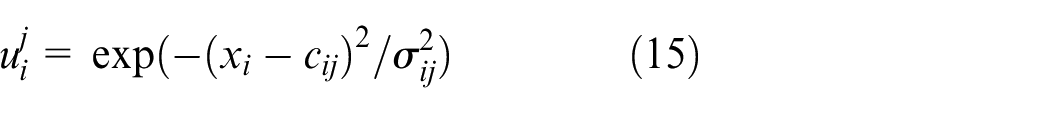
where
The iteration of the hybrid learning algorithm consists of two steps. The first step aims to fix the parameters of the antecedent
In the second step, the obtained error signal is propagated back into the network, and the BP algorithm is used to adjust the parameters of the antecedent. Using the hybrid learning algorithm with a given predecessor parameter, the global set of the post-parameter parameters can be obtained. This step can not only reduce the dimension of the search space in the gradient descent method but also significantly improve the convergence speed of the parameter.
To train the model, the acquired wavelength data were fed to the fuzzy neural network and 50 sets of training mode data were determined. After the preprocessing, the learning samples were created to train the network, in which the network was trained using a set of input modes and a corresponding set of output modes was obtained as training samples. The training process served as the conditioning process of network parameters and structures.
As for the network parameters, the learning rate was set to 0.15 and the maximum number of iterations was 700 and the error was set to 0.02. The root-mean-square error gradually converged with the number of iterations. When the iteration number exceeded 518 times, the root-mean-square error started to be stabilized, indicating that the model has been effectively trained. The training error curve is shown in Figure 6. After the network training completed, a fuzzy neural network strain identification model was established.
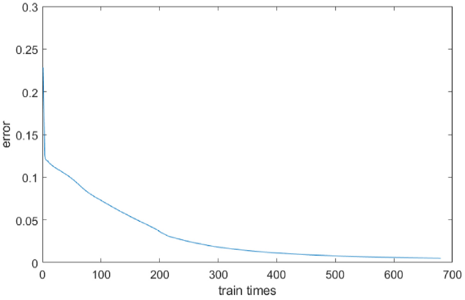
Errors of training samples.
Experimental results and discussion
The spectral features, including the resonance wavelength (λ) and the amplitude (λp) at the resonance wavelength, were found using the measured transmission spectra as shown in Figure 5. The λ, λp, and ϵ data points can be fitted using polynomial regression. The relationships between spectral features and the axial strain, λ(ϵ) and λp(ϵ), were obtained by linear fitting equations. With the increasement of the load, the axial strain of LPFG also increased, and thus the λ and λp values changed accordingly. The increase in axial strain shifted the λ to a shorter wavelength and, in the meantime, the λp value increased.
The change of λ as a function of axial strain follows the fitting equation of
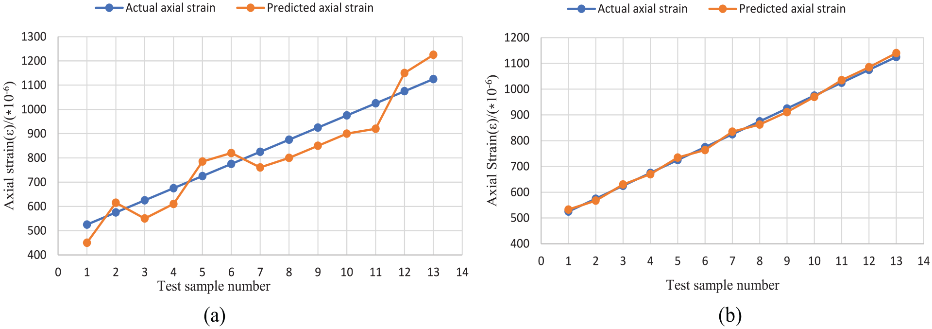
Comparison of two methods’ predicted strain using (a) the linear fitting algorithm and (b) the ANFIS model.
When the entire network is successfully trained, the learning results are stored in the antecedent parameters and the post-parameter parameters. At the end of the network learning process, the network output is calculated using the previously stored parameters. The purpose of this step is to test the efficiency of the network learning. The learning result determines the quality of the calculated output. Based on the measured λ and λp data, the axial strain value can be predicted using the trained ANFIS.
In Figure 8, the relative error rates between the predicted and actual values of the axial strain are marked. The relative error rates are from −14.29% to +8.89% using the linear fitting algorithm, and the R-squared statistics is 0.8815. In contrast, the relative error rates of the axial strain predicated by the ANFIS model are from −1.5% to 1.43%, and the R-squared statistics is 0.9872. There are several sources of error, such as notch effect caused by glue sticking, cross sensitivity of environmental factors, accuracy of instruments, and so on.
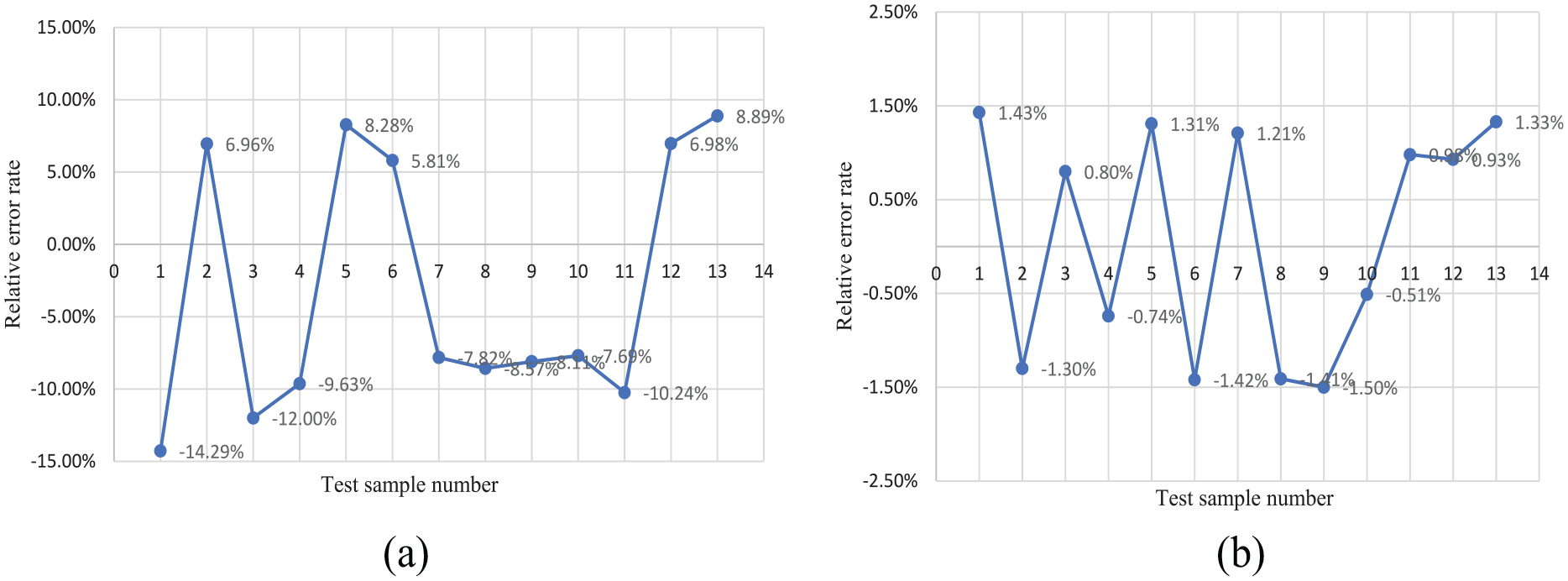
Comparison of two methods’ relative strain error using (a) the linear fitting algorithm and (b) the ANFIS model
After the learning process, the fuzzy neural network model can still give a correct input–output relationship for non-training samples in the same sample set. By comparing Figures 7 and 8, it can be seen that the ANFIS model exhibits an improved prediction accuracy. Importantly, the ANFIS predicted that the axial strains are closer to the actual strained values than the linear fitting method.
The proposed ANFIS model is a multi-input single-output inference system. The model uses a fuzzy logic system for neural network calculation and learning to determine the parameters of the network membership functions, obtain fuzzy rules, and improve the neural network learning ability. The results show that the ANFIS model can effectively improve the accuracy of strain quantification compared with the conventional data fitting method.
Conclusion
In this paper, the ANFIS model has been successfully developed to investigate the correlations between the axial strain and the spectral features of the LPFG sensor outputs. The performance of the ANFIS model was compared to that of the data fitting methods. The relative error rates of the axial strain predicated were in the range ±1.5% in the case of the ANFIS model, while they were in the range ±14.29% in the case of the linear fitting algorithm. The results showed that the application ANFIS model can enable strain quantification with higher accuracy compared with the conventional data fitting methods. The model is built upon the qualitative knowledge and the ability to self-learn to process spectral data acquired from the LPFG sensor and output strain values with high precision. Moreover, the developed network learning model can be accomplished after a few learning cycles using the measured LPFG spectral features. It is also worth noting that the developed ANFIS model is highly versatile and can be applied to other sensing applications with minor modifications.
Footnotes
Declaration of conflicting interests
The author(s) declared no potential conflicts of interest with respect to the research, authorship, and/or publication of this article.
Funding
The author(s) disclosed receipt of the following financial support for the research, authorship and/or publication of this article: This research was funded by the General Program of Jiangsu Province’s Natural Science Foundation under grand BK20171114, Qing Lan Project and Jinling Institute of Technology’s Talent Introduction Project under grant Jit-rcyj-201604.