
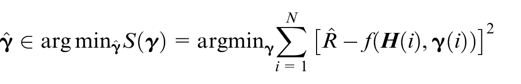
Abstract
In order to improvethe yaw angle accuracy of multi-rotor unmanned aerial vehicle and meet the requirement of autonomous flight, a new calibration and compensation method for magnetometer based on Levenberg–Marquardt algorithm is proposed in this paper. A novel mathematical calibration model with clear physical meaning is established. “Hard iron” error and “Soft iron” error of magnetometer which affect the yaw accuracy of unmanned aerial vehicle are compensated. Initially, Levenberg–Marquardt algorithm is applied to the process of sphere fitting for the original magnetometer data; the optimal estimation of sphere radius and initial “Hard iron” error are obtained. Then, the ellipsoid fitting is performed, and the optimal estimation of “Hard iron” error and “Soft iron” error are obtained. Finally, the calibration parameters are used to compensate for the magnetometer’s output during unmanned aerial vehicle flight. Traditional ellipsoid fitting based on least squares algorithm is taken as reference to prove the effectiveness of the proposed algorithm. Semi-physical simulation experiment proves that the proposed magnetometer calibration method significantly enhances the accuracy of magnetometer. Static test shows that the yaw angle error is reduced from 1.2° to 0.4° when using the proposed calibration model to calibrate magnetometers. In dynamic tests, the sensor MTi’s output is used as reference. The data fusion of magnetometer compensated by the proposed new calibration model based on Levenberg–Marquardt algorithm can accurately track the desired attitude angle. Experimental results indicate that the accuracy of magnetometer in the yaw angle estimation has been greatly enhanced. In the process of attitude estimated, the compensation magnetometer data given by this new method have faster convergence speed, higher accuracy, and better performance than the compensation magnetometer data given by traditional ellipsoid fitting based on least squares algorithm.
Introduction
In recent years, with the development of unmanned aerial vehicle (UAV) technology, UAV has been widely used in various fields. In autonomous flight of UAV, the accuracy and stability of yaw angle directly affect the accuracy of navigation. The electronic magnetic compass has the advantages of small size, low cost, fast dynamic response, and no cumulative error, and is widely used in the navigation system of UAV to provide the yaw angle. 1 However, its accuracy is easily affected by surrounding magnetic field environment and electrical layout of the UAV itself. To improve the accuracy of the yaw angle estimation, the magnetometers should be calibrated again before takeoff. 2 Therefore, magnetometer calibration and compensation have become a research hotspot.3,4
Many research teams have made outstanding contributions in the fields of magnetometer calibration. Sun and Fang 5 used multi-sensor information to compensate and filter the output information of inertial instruments such as magnetic compass and global positioning system (GPS) to calibrate the measured value of the magnetic sensor, which has online real-time compensation capability. Yan et al. 6 analyzed the singularity of the coefficient matrix; the least squares method was used to identify the error coefficients of the elliptic model, overcoming the instability and suppressing the sudden disturbance in the calibration process. Fang et al. 7 proposed a magnetic compass calibration method based on the constrained least squares ellipsoid fitting, while it can only be used in the absence of magnetic interference. Pang et al. proposed an improvement of magnetometer calibration using Levenberg–Marquardt (L-M) algorithm. The L-M algorithm is applied to traditional ellipsoid fitting to estimate the calibration parameters and proved that the L-M algorithm is a good method for magnetometer calibration. 8
Most previous researchers have used two methods to calibrate magnetometer separately: the classic independent ellipsoid fitting method and the independent sphere fitting method. Traditional methods mainly aim at the calibration of pure magnetometer. To obtain more accurate calibration parameters on UAV, a new calibration model according to UAV’s magnetic field environment and the calibration process of magnetometer is completed on UAV. According to the magnetic field characteristics of UAV, this paper innovatively combines the traditional sphere fitting and ellipsoid fitting algorithm, and proposes a new magnetometer calibration model, which can be used to compensate the “Hard iron” error and “Soft iron” error of magnetometer on multi-rotor UAV. In the first step, the L-M algorithm is used to fit the original magnetometer data into a sphere, and the optimal estimation of sphere radius and initial “Hard iron” error are obtained. In the second step, the L-M algorithm is applied to the process of the ellipsoid fitting to calculate the optimal estimation of “Hard iron” error and “Soft iron” error. The estimated parameters obtained by the sphere fitting are used as the initial value of the ellipsoid fitting. The proposed calibration method can estimate the “Hard iron” error and the “Soft iron” error of UAV more accurately, and the residual errors of compensated magnetometer data are smaller and the fitting performance is better. It is insensitive to the initial value. The calibration process is simple, and no external auxiliary equipment is needed. There are not any requirements in the direction and angle during the rotation. In the process of UAV attitude estimation, the convergence speed is faster, the convergence accuracy is higher, and the stability is better.
The main contributions of this research can be summarized as follows:
An improved magnetometer calibration method of the sphere fitting and the ellipsoid fitting is proposed in this paper. A novel mathematical calibration model with a clear physical meaning is established.
The L-M algorithm is applied to the process of the sphere fitting and the ellipsoid fitting simultaneously, and a semi-physical experimental system was designed for the simulation experiments.
An UAV experimental platform based on STM32F429 hardware platform is built. Dynamic and static experiments are designed to verify the validity of the calibration method, and the least squares (L-S) algorithm is used as a comparison.
Error source of magnetometer
The intention of a magnetometer in a compass application is to measure Earth’s magnetic field. Measurements other than those of Earth’s magnetic field are considered as errors.9,10 The purpose of the magnetometer calibration is to calculate a set of correction parameters that compensate for various source errors: sensor zero deviation, scale-factor error, horizontal axis sensitivity, “hard iron” error, and “soft iron” error.4,11 Sensor zero bias, scale-factor error, and cross-axis sensitivity are the sensor’s self-error, and they were calibrated before the sensors leave the factory.
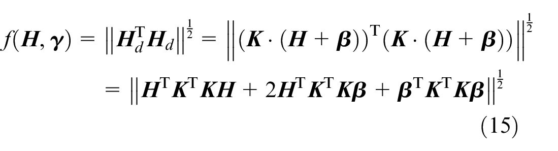
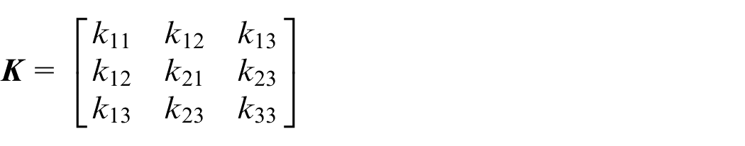
When the magnetometer is used in UAV, it will be affected by the motor and the surrounding magnetic field environment. 12 The errors of disturbing magnetic field mainly include “Hard iron” error and “Soft iron” error. The magnetometer needs to be calibrated again before the UAV takes off.13,14“Hard iron” error is caused by materials fixed to the vehicle body that produces static magnetic fields. “Soft iron” error is caused by materials fixed to the vehicle body that distorts magnetic fields.15,16 The proposed algorithm computes a set of correction parameters that compensate for errors from “Hard iron” error and “Soft iron” error.
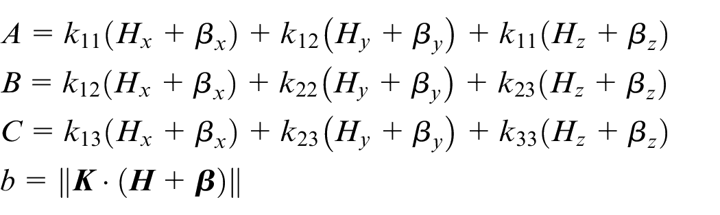
The error model can be described as

where
“Hard iron” error and “Soft iron” error can be obtained by taking a set of samples that are assumed to be the product of rotation in Earth’s magnetic field and fitting an offset ellipsoid to them, determining the correction to be applied to adjust the samples into an origin-centered sphere. 17
The L-M algorithm for sphere and ellipsoid fitting
The L-M algorithm combines the advantages of steepest descent method and Newton method. It is often used to solve the minimum value problem of the sum of squares of functions.18,19 This algorithm is applied to the sphere and the ellipsoid fitting of magnetometer measurement data to obtain “Hard iron” error and “Soft iron” error.
The total intensity of Earth’s magnetic field that is measured by an ideal magnetometer should be a constant, which is mathematically described to be
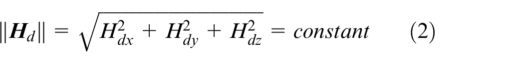
where
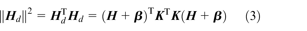
According to equation (3), it is constrained by a positive sphere or ellipsoid, which can be written in the following form
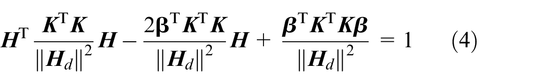
The shifted origin indicates the existence of “Hard iron” error, and the changed shape indicates the existence of “Soft iron” error.
Repeated measurements show that the original data of magnetometer are roughly distributed on a sphere, indicating that the UAV is mainly affected by “Hard iron,” while the “Soft iron” error is relatively small. In fact, it is an ellipsoid, but it is very similar to a normal sphere. According to the practical engineering problems, we adopt the sphere hypothesis to solve the problem of magnetometer calibration for UAV. First, sphere fitting is performed and “Hard iron” error is estimated, and the optimal estimation of sphere radius R is performed using the L-M algorithm. In the second step, we continue to collect the magnetometer data, do an ellipsoid fitting, and use the radius R of the first sphere fitting as the convergence criterion of ellipsoid fitting, and estimate “Soft iron” error effectively based on the sphere hypothesis. The R is applied to ensure whether the conicoid is a sphere.
Step 1: the sphere fitting
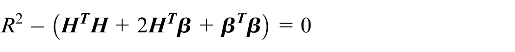
The sphere fitting method based on the L-M algorithm only takes “Hard iron” error into consideration. The error model was summarized as follows

Assuming that the radius of the sphere is R. According to equation (3)

A function is introduced
The primary application of the L-M algorithm is in the least squares curve fitting problem: given a set of N empirical datum pairs
The L-M algorithm is an iterative method that requires an initial parameter
where
In order to complete the iterative process, the Jacobian matrix

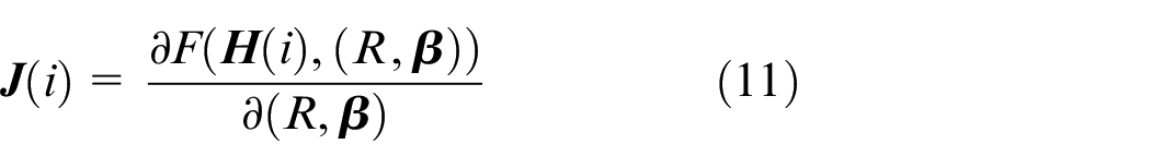
Suppose the total number of magnetometer samples is N. According to equations (6) and (10), the error equation of the sample i is
So the Jacobian matrix is
So the Jacobian for N samples is

The initial value
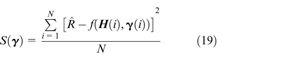
After each iteration, the squared residual sum of all samples was calculated
The direction of each exploration is the direction of decreasing the value of
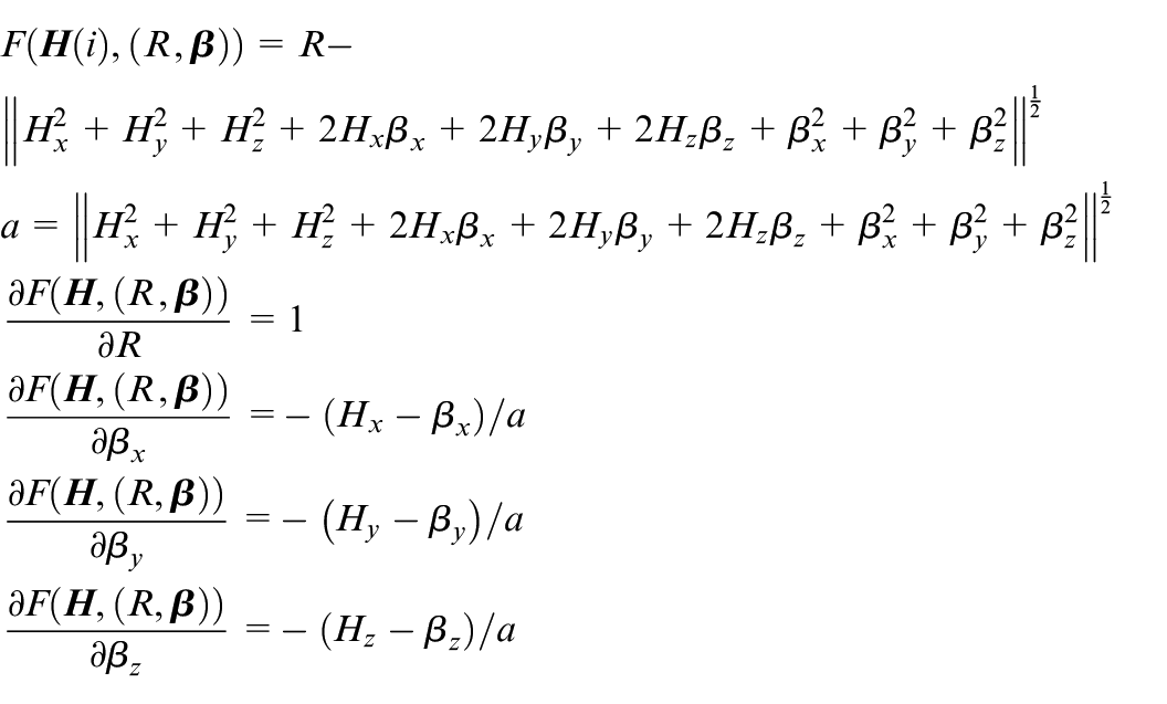
Step 2: ellipsoid fitting
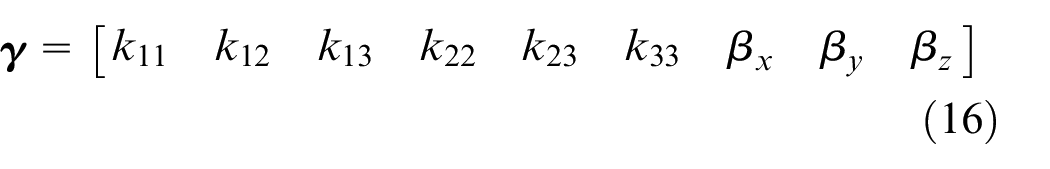
The ellipsoid fitting method based on the L-M algorithm takes “Hard iron” error and “Soft iron” error into consideration and obtains their optimal estimation. The optimal radius
Find the optimal estimation of the parameters
where
where
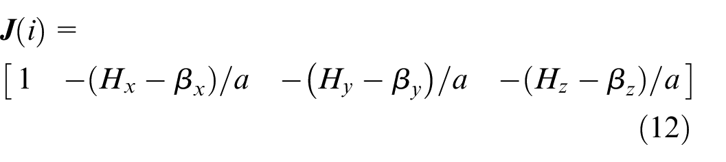
According to the process of the L-M algorithm, calculate Jacobian matrix
Similar to the sphere fitting, the Jacobian matrix of the ellipsoid fitting is given directly
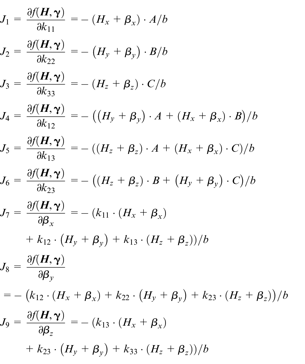
So the Jacobian for N samples is

Jacobian matrix
The initial value of
After the convergence accuracy is satisfied, the optimal
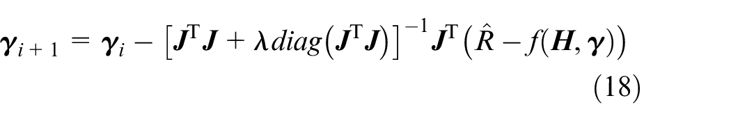
The iteration process of the L-M algorithm and choice of
parameter
Taking the sphere fitting as an example, the iteration steps are explained;
The iteration steps of the L-M algorithm for sphere fitting are shown in Figure 1.
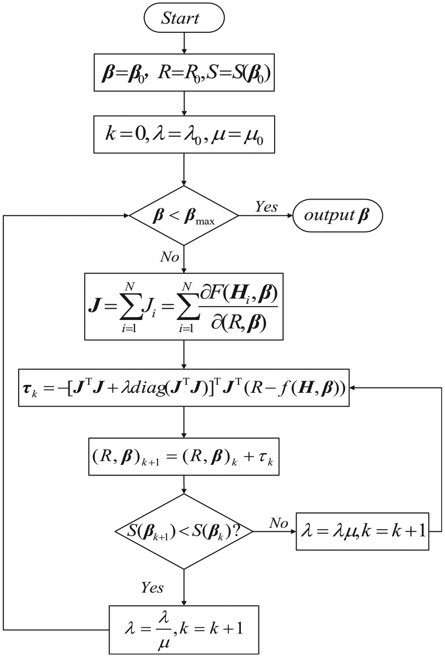
The iteration steps of the L-M algorithm for sphere fitting.
At the beginning of the iteration, take
Magnetometer calibration process
Magnetometer calibration includes the sphere fitting and the ellipsoid fitting. Rotate the magnetometer in Earth’s magnetic field. Once the sample buffer is full, a sphere fitting algorithm is run, which computes a new sphere radius and “Hard iron” error until the acceptance criteria are met. Samples were collected until the buffer is full again, and the ellipsoid fitting algorithm is run. The sphere radius and “Hard iron” error obtained by the sphere fitting process are taken as the initial values to enter the ellipsoid fitting process. The ellipsoid fitting computes “Soft iron” error, and the corrected “Hard iron” error is carried out. The fitting process is shown in Figure 2.
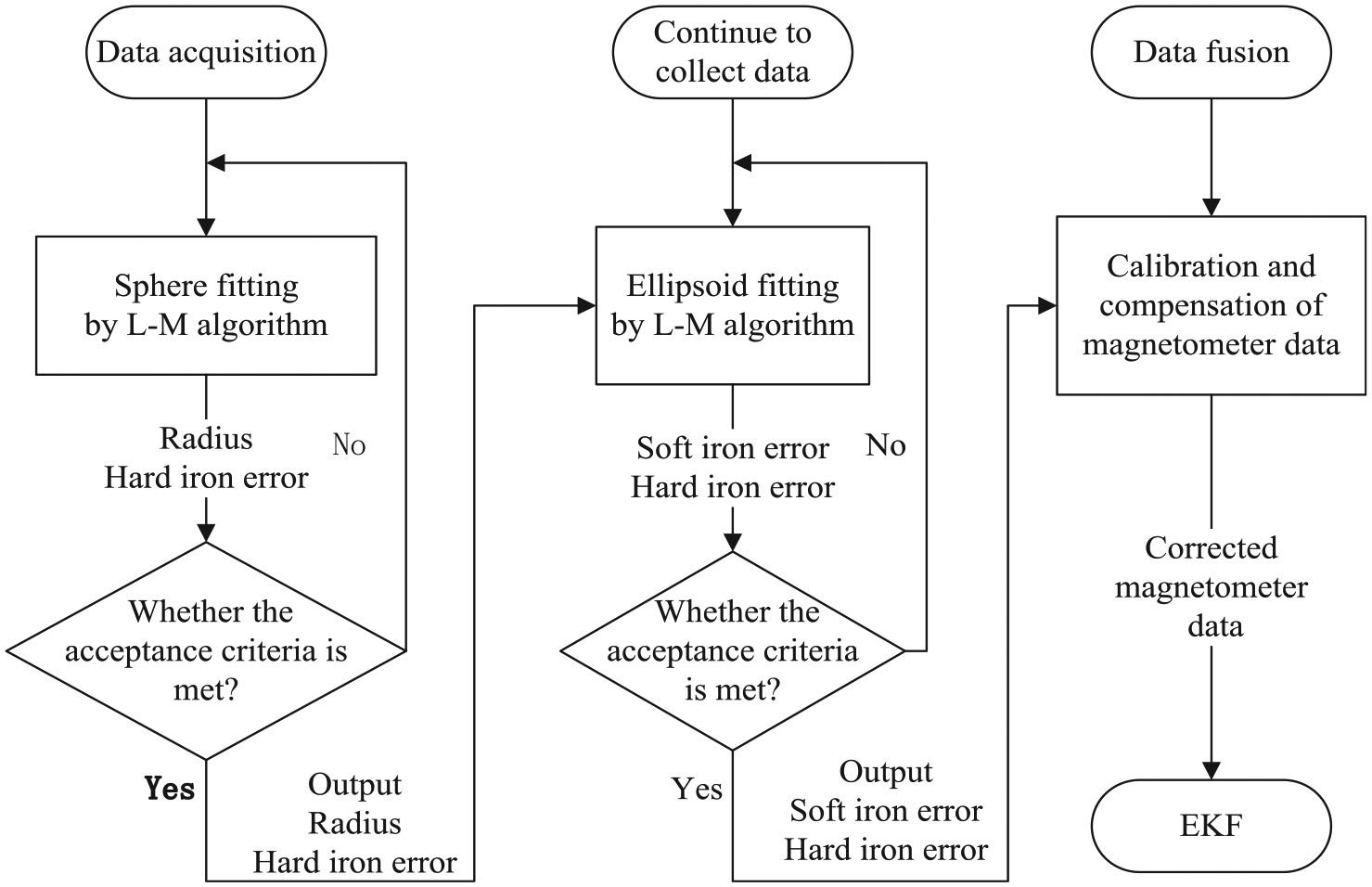
Flowchart for the calibration and compensation.
Experiments and results
Real measured data are used in this paper to verify the performance of the L-M algorithm for magnetometer calibration. The UAV was rotated to collect original magnetometer data, and then the original data of the magnetometer were imported into the pre-written magnetometer calibration MATLAB program to calculate the “Hard iron” error and “Soft iron” error.
Magnetometer calibration
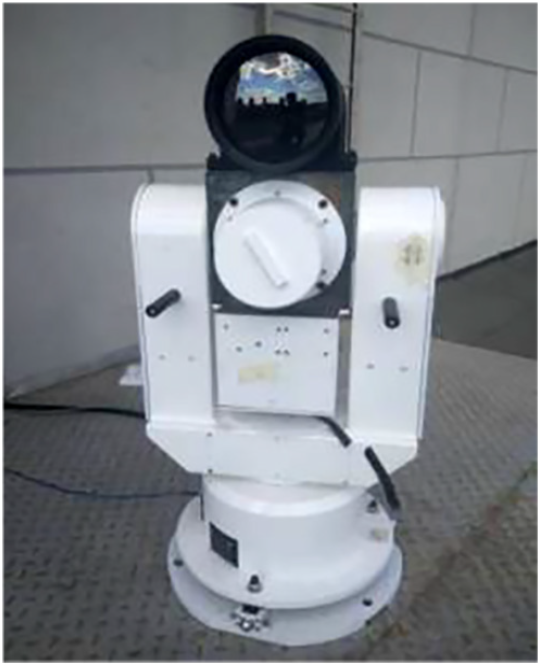
The magnetometer LSM303D is fixed on the multi-rotor UAV, as shown in Figure 3. The navigation coordinate system is the north-east coordinate system. The body coordinate system is defined at the origin of UAV: X-axis points to the front, Y-axis points to the right, and Z-axis points to the bottom. The UAV is rotated for several times along its X, Y, and Z axes at a constant speed. The collected magnetometer original data are returned to the computer through the serial port. The original data are added into the standard L-S algorithm and the L-M algorithm for MATLAB file. The initial iteration parameters of the L-M algorithm are shown in Table 1. About 2000 pieces of original data were collected. The three-dimensional (3D) data figure of the original value of the magnetometer and the magnetometer compensated by the L-M algorithm are shown in Figure 4, and those by the L-S algorithm are shown in Figure 5.
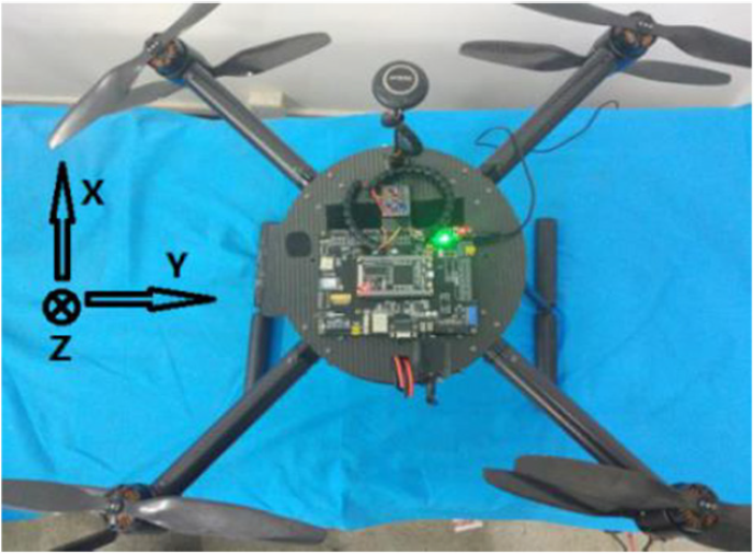
The hardware platform of UAV.
The initial iteration parameters of the L-M algorithm.
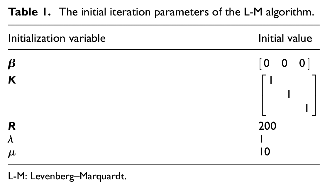
L-M: Levenberg–Marquardt.
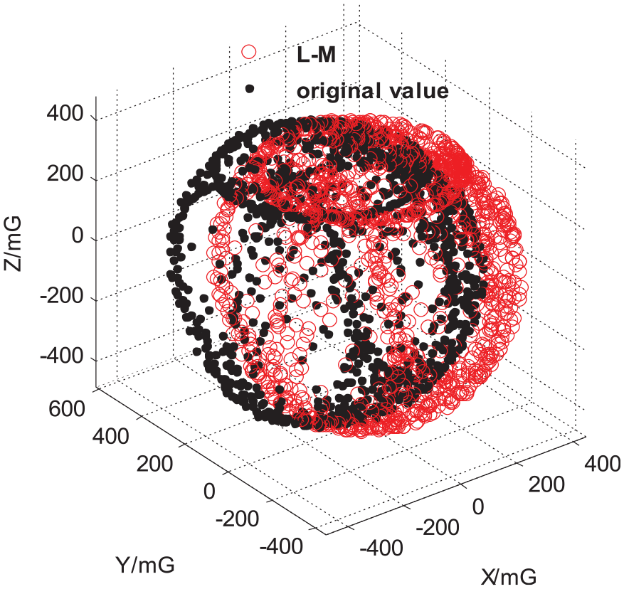
The 3D graph of original data and compensation data by proposed L-M algorithm
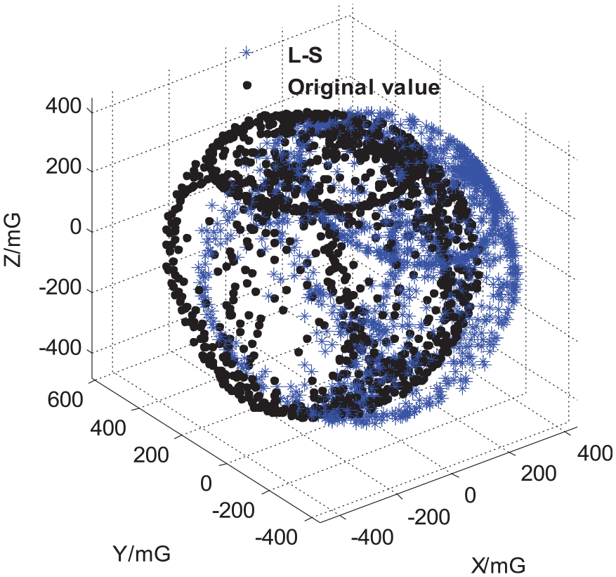
The 3D graph of original data and compensation data by traditional L-S algorithm.
Both algorithms can estimate the “Hard iron” error and “Soft iron” error. The optimal estimation parameters are shown in Table 2. As for “Hard iron” error compensation, the results of the two algorithms are similar. Figures 6 and 7 show that all of the magnetometer sample data have a perfect circle centered at the origin in the projection plane of X–Y, Y–Z, and Z–X. The correction was applied to adjust the samples into an origin-centered sphere. The main difference between the two algorithms is the parameter of the “Soft iron” error
The “Hard iron” error and “Soft iron” error estimated by the L-M and the L-S algorithms.
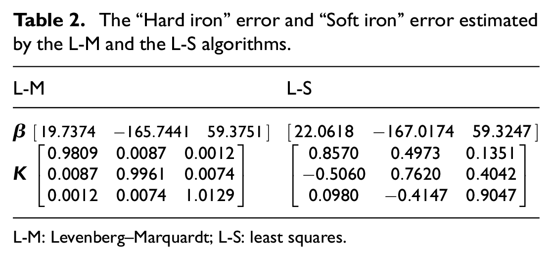
L-M: Levenberg–Marquardt; L-S: least squares.
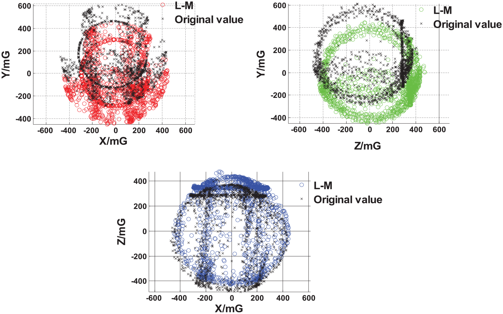
The projection plane of X–Y, Y–Z, and Z–X of original data and compensation data by the L-M algorithm.
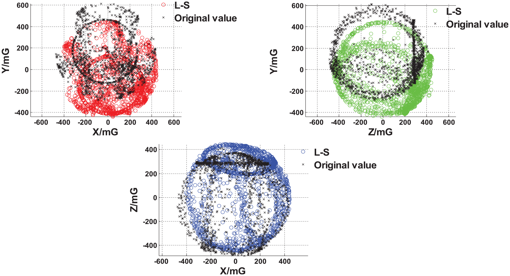
The projection plane of X–Y, Y–Z, and Z–X of original data and compensation data by the L-S algorithm.
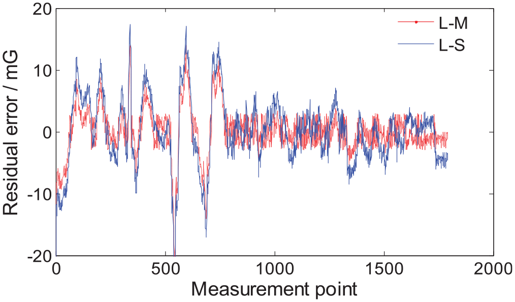
The residual error with the proposed calibration based on the L-M algorithm and traditional ellipsoid fitting based on the L-S algorithm are shown in Figure 8. The residual error before calibration is shown in Figure 9. It can be seen that both the algorithms have good performance in calibration. The residual error is reduced from 200 to 20 mG, and the residual error with the L-M algorithm is smaller than that with the L-S algorithm.
Residual error with the proposed L-M algorithm and traditional L-S algorithm.
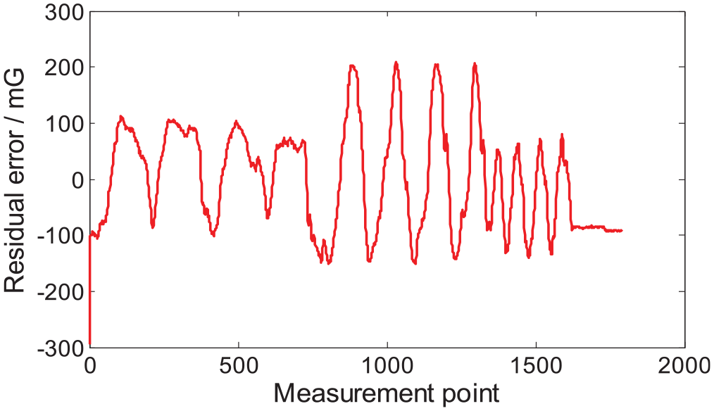
Residual error before calibration.
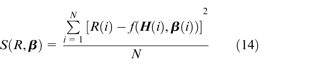
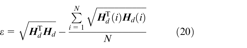
In total, 10 repetitive experiments were conducted to prove the effectiveness of the proposed algorithm. The performance of these two calibration methods is evaluated by the mean of the residual error for all data

The list of the
The list of the
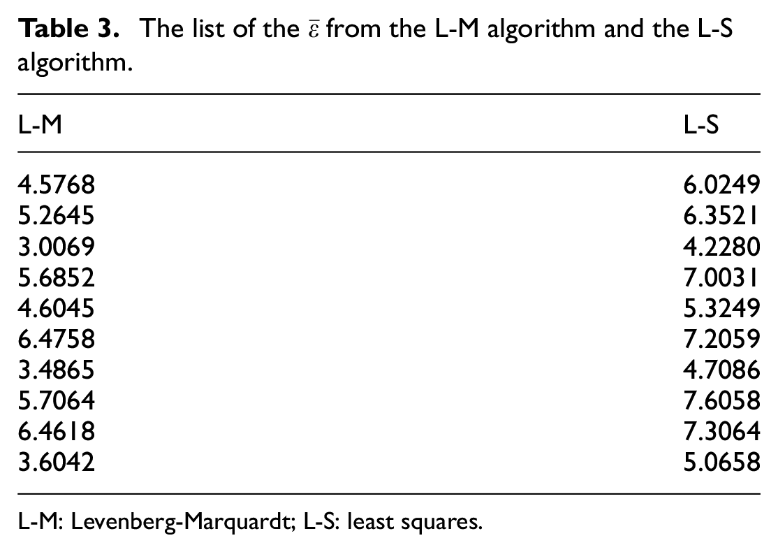
L-M: Levenberg-Marquardt; L-S: least squares.
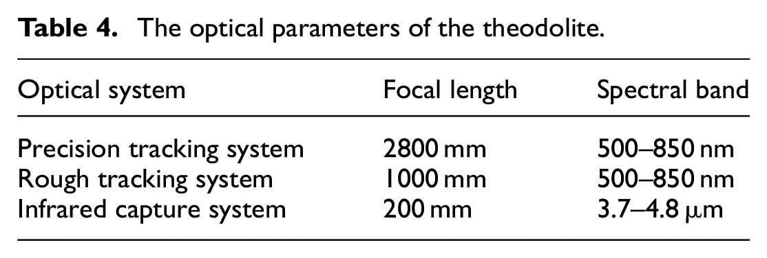
A semi-physical experimental system was designed for the simulation experiments. The measure system was testified by triaxial theodolite as shown in Figure 10, which is supported by Changchun Institute of Optics, Fine Mechanics and Physics, Chinese Academy of Sciences. Theodolite is an optical aiming and tracking device, which can be used to observe and record the flight trajectory and attitude of various aircrafts. The system can achieve 2″ high-precision tracking. The whole system consists of precision tracking system, rough tracking system, and infrared capture system. The optical parameters of each part of the system are shown in Table 4.
Triaxial theodolite.
The optical parameters of the theodolite.
The theodolite with three degrees of freedom was used to provide a resolution of 0.01° for the yaw angle. Figure 11 shows the yaw angle errors after calibration by the proposed calibration based on the L-M algorithm and traditional ellipsoid fitting based on the L-S algorithm. It was apparent that the proposed improved magnetometer calibration and compensation method based on the L-M algorithm significantly enhanced the accuracy of the magnetometer.
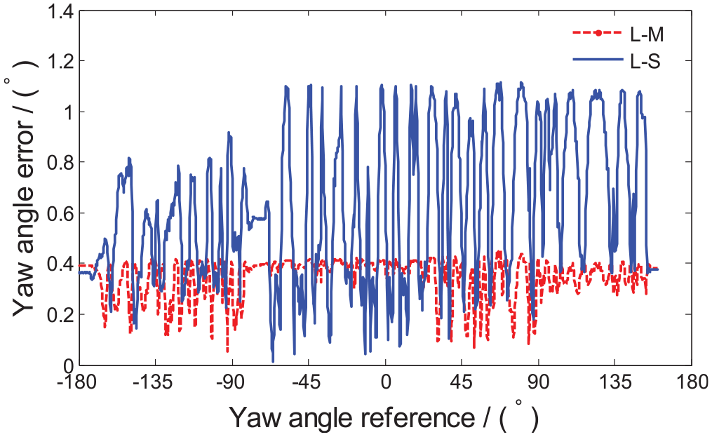
The yaw angle error after calibration.
To further evaluate the performance of the calibration algorithm, a double-sensor hardware platform is built. One group of sensors is based on STM32F429, which includes accelerometer and gyroscope MPU6000, and magnetometer LSM303D. The standard extended Kalman filter (EKF) attitude estimation method is integrated into this hardware platform, and the attitude angle is outputted in real time. Another group of sensors adopts the MTi inertial measurement unit (IMU) produced by Xsens in the Netherlands, which has its own EKF algorithm and can directly output high-precision attitude angle. The precision of the roll angle and the pitch angle in the algorithm is ±0.3°, and the precision of the yaw angle is ±0.5°. The product provides high-quality orientation and position, which belongs to the high-performance IMU.
The attitude angle of MTi is used for control of the UAV. The EKF algorithm integrated in STM32F429 is only used to estimate attitude angle but the estimated states are not used for control of the UAV. All the flight data, including the measured sensor data and attitude angle, are stored in the flight control unit.
Static test
Place the UAV on the horizontal ground with the nose facing due north, theoretically maintaining a zero-degree angle. The compensation parameters of proposed L-M algorithm and traditional L-S algorithm are written into magnetometer original data. The calibrated data are added to the EKF algorithm of magnetometer data fusion to calculate the attitude angle in real time. EKF used for the estimation of the yaw angle by fusing magnetometer data does meet the situation: the better the calibration, the better the final result. The test time is about 280 s. The comparison between the L-M’s output and the L-S’s output is shown in Figures 12 and 13.
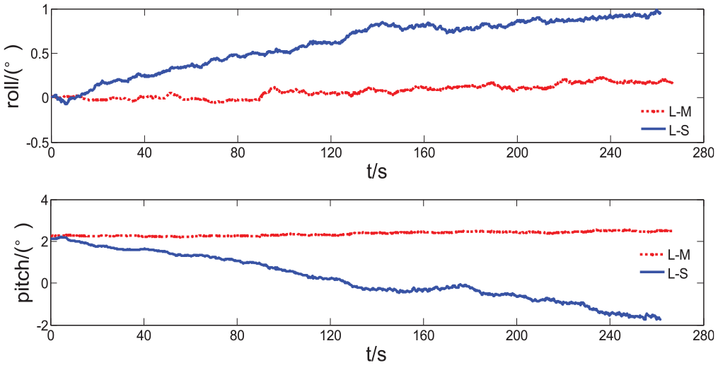
The comparison of roll angle and pitch angle.
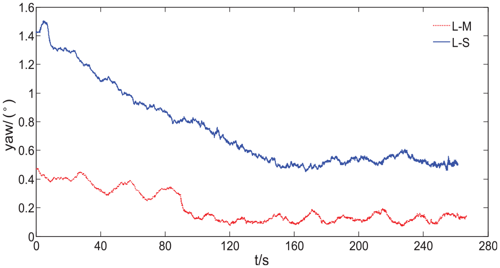
The comparison of the yaw angle.
The static test results show that the performance of the pitch angle and the roll angle of the magnetometer data compensated by the L-M algorithm and fused by the EKF algorithm is better. Because the ground cannot maintain strict horizontal, there are different degrees of small angle values for the roll angle and the pitch angle. Initial alignment is given by the accelerometer value, so the roll angle and the pitch angle start from the same initial value. Magnetometer data fusion will correct them; after a period of time, they stabilize around the initial value with accuracy within 0.5°. However, the angle with the L-S algorithm is gradually far away from the initial value and has a large error compared to the real value.
Static test results of the yaw angle are shown in Figure 13, and the initial value compensated by the L-M algorithm is 0.45° and by the L-S algorithm is 1.4°. The initial value of the L-M algorithm is closer to the true value, which converges to 0.18° over time, while the L-S algorithm converges to 0.6°. The L-M algorithm has a shorter convergence time than the L-S algorithm. The static accuracy of yaw angle of the L-M algorithm is within 0.2° and that of the L-S algorithm is within 0.6°. It indicates that the L-M algorithm has short convergence time and high convergence accuracy. The dynamic accuracy usually depends on the initial accuracy of the yaw angle, so it can be judged that the L-M algorithm has higher dynamic accuracy of the yaw angle.
Dynamic test
In order to verify the dynamic accuracy of the algorithm, UAV flies along a high-maneuvered trajectory with a flight time of approximately 1000 s. The UAV conducts autonomous flight along a circular trajectory. Take the take-off position of the UAV as the origin and record the location of every moment during the flight. The attitude angle output of the MTi IMU guides the flight and serves as a reference. The 2D (two-dimensional) trajectory and the 3D trajectory of the flight test are shown in Figures 14 and 15.
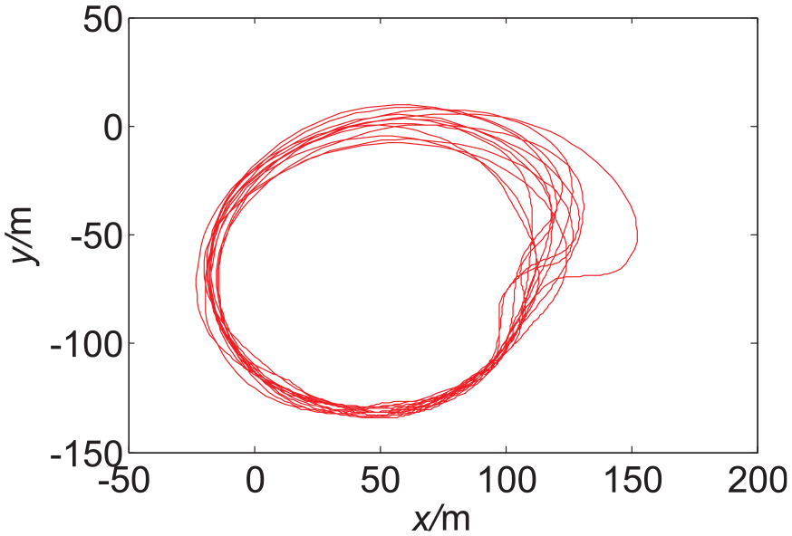
The 2D trajectory during the flight test.
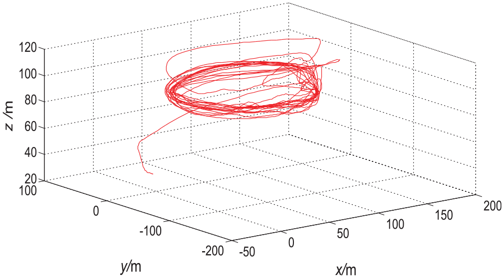
The 3D trajectory during the flight test.
The performance of roll angle and pitch angle compared with MTi’s output is shown in Figure 16. As seen from the figure, for both the L-M algorithm and the L-S algorithm, the roll angle and pitch angle can accurately track the attitude angle output by the MTi sensor. High-precision solution can be maintained under frequent large-angle movement, and attitude tracking has good real-time performance.
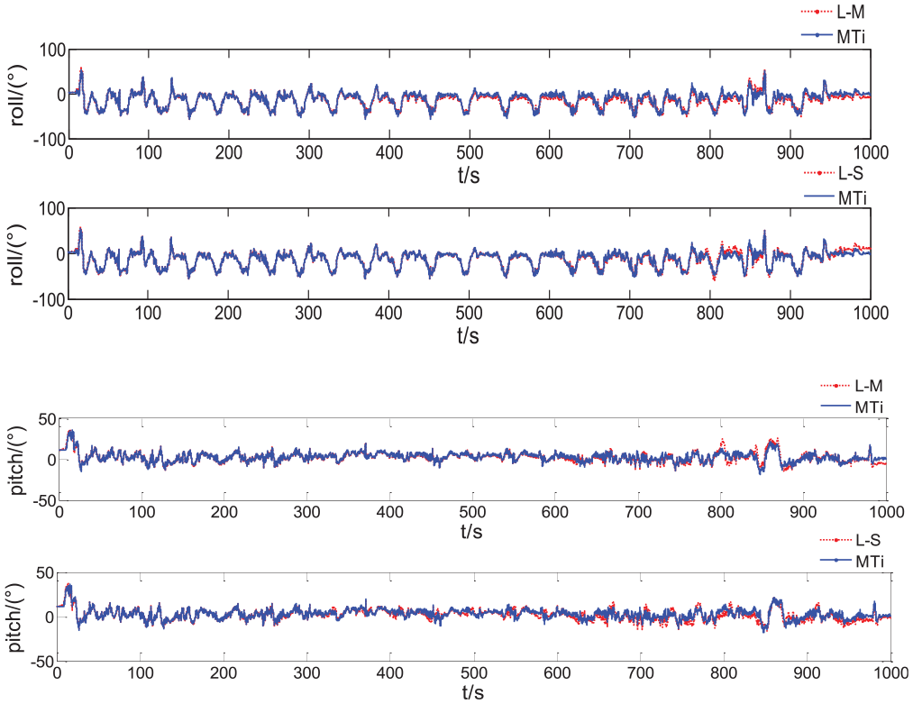
Comparison of roll angle and pitch angle to MTi’s output.
The performance of the yaw angle is shown in Figure 17. The L-M algorithm could track the desired angle with high precision, and has high reliability and stability. However, the L-S algorithm performed better at the beginning. At the flight time of 320 s, the yaw angle began to show the hysteresis phenomenon, which became more and more serious. Divergence occurred at 700 s, and the yaw angle could not accurately track the desired angle. The reason for this phenomenon is that the L-S magnetometer calibration algorithm fails to perform a good calibration of the original value of the magnetometer. As a result, the magnetometer data added to the EKF attitude estimation algorithm are mixed with a lot of noise, which leads to errors between the estimated attitude angle and the real value. EKF is an iterative algorithm, and the error of attitude angle will accumulate with the increase of iteration number, so the divergence phenomenon of the yaw angle is caused.
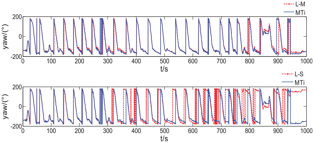
Comparison of the yaw angle to MTi’s output.
Conclusion
This paper proposes an improved magnetometer calibration method based on the L-M algorithm. The “Hard iron” error and the “Soft iron” error, which affect the yaw accuracy, are calibrated by the sphere fitting and the ellipsoid fitting, and then the optimal parameters of “Hard iron” error and “Soft iron” error are obtained. Semi-physical simulation experiment proves that the proposed magnetometer calibration method significantly enhances the accuracy of the magnetometer. To further evaluate the performance of the calibration algorithm, the performance of the L-M algorithm is verified by the measured magnetometer data from UAV. Traditional L-S ellipsoid fitting algorithm is taken as reference. The tests include static test and dynamic test, and the dynamic test uses MTi sensor’s output as reference. Static test shows that the accuracy of the yaw angle is within 0.4° when using the L-M algorithm to calibrate magnetometer. The accuracy of attitude angle estimated by EKF algorithm is quite comparable with that of MTi attitude angle output. At the same time, the traditional ellipsoid fitting method based on the L-S algorithm is also comparable with the L-M algorithm. The L-M algorithm is better than the L-S algorithm when applied to the ellipsoid fitting to compensate magnetometer data. In this paper, a precise, stable, and efficient field calibration method of UAV magnetometer is provided. The method proposed in this paper not only solve the problem that magnetometer calibration accuracy is not high but also obviously improve the convergence rate of attitude angle of magnetometer data fusion.
Footnotes
Acknowledgements
The authors thank Changchun Institute of Optics, Fine Mechanics and Physics, Chinese Academy of Sciences for supporting the research.
Declaration of conflicting interests
The author(s) declared no potential conflicts of interest with respect to the research, authorship, and/or publication of this article.
Funding
The author(s) disclosed receipt of the following financial support for the research, authorship, and/or publication of this article: This work is supported by the National Natural Science Foundation of China (grant nos 11372309, 61304017), Jilin Province Science and Technology Development Program (grant nos 20150204074GX, 20160204010NY), Provincial and Academic Cooperation Science and Technology Special Fund (grant no. 2017SYHZ0024), and Chinese Academy of Sciences Youth Promotion Program (grant no. 2014192).