
Abstract
The electronic speed governor plays an important role in diesel generator sets. The ideal method for developing and debugging the electronic governor is to simulate the diesel engine’s dynamic characteristics with the hardware-in-the-loop simulation system. In this system, the diesel engine can be replaced by a mathematical model. Our research proposed a novel diesel engine modeling method using the long short-term memory neural network for simulating dynamic characteristics of the rotational speed of diesel generator sets. The proposed model is trained and tested on the data of the real diesel generator sets. With different power loads and unloads, experimental results demonstrated that this method was able to successfully simulate the dynamic characteristics of diesel generator sets. In addition, comparing to other existing methods provided a conclusion that the performance of the model was better than others. Finally, the proposed model was deployed on an established hardware-in-the-loop simulation system. The results further demonstrated that this model was able to reproduce the diesel generator sets’ dynamic characteristics.
Introduction
Diesel generator sets (DGS) as an important power source has been applied in many fields, for example, emergency system, mobile power station, marine electrical power plate, and agriculture.1–3 In alternating current (AC), power generation system, the power frequency is proportional to the diesel engine’s rotational speed. Therefore, the electronic speed governor is a very important part since it controls the rotational speed of DGS. For a DGS, the quality of AC power outputs largely depends on the performance of the electronic speed governor. Generally, each speed governor is required to be adjusted and tested on each real DGS. However, this process is not cheap and produces large amounts of emission.4,5 To solve those problems, the ideal way is to take advantage of a hardware-in-the-loop (HIL) simulation system for simulating the dynamic characteristics of the rotational speed in DGS; then, the electronic speed governor can be developed and validated on this platform. 6
In a HIL system, the significant component is the diesel engine model. 7 It is responsible for simulating and reproducing the dynamic characteristics of a diesel engine. To be specific, this model has an ability to reflect the relationship between the inputs, that is, power loads and the rack of displacement, and the rotational speed output. According to our investigations, the existing modeling methods of diesel engine mainly contain two types of models. The first one can be regarded as mechanism modeling, the second one as system identification.
Mechanism modeling method needs enough professional kinematical and thermodynamic knowledge about the diesel engine.8–10 Specifically, one diesel engine has a variety of complicated dynamic processes including intake, fueling, combustion, power production, heat release, heat transfer, and exhaust. Therefore, it is very hard to create a precise mathematical model for diesel engine. To reduce the dimensions of complexity, most of researchers consider to make the model simplification and give some hypotheses, such as quasi-steady state, linearization model, and filling-and-emptying model.11,12Although this type of model can accurately reflect the static and dynamic characteristics, its high computation cost makes it very difficult to be used as a modeling method for the HIL simulation system because of real-time requirement.13,14
System identification is thought as a black box modeling method, which takes advantage of the input and output information to build a model for a dynamic system. Liu et al. 15 built a single-input single-output model with nonlinear auto regressive mode with exogenous (NARX) method to simulate the rotational speed of a diesel engine. However, the relationship between rotational speed and power loading conditions was not considered in this system. Jiang et al. 17 and Ai et al. 16 also used the NARX technique to build a diesel engine model. This method gave the impact of the power loading and unloading conditions on the diesel engine models. In addition, they successfully deployed the proposed model on an established HIL simulation system of DGS. Artificial neural network (ANN) has been regarded as a useful modeling method for the diesel engine research, for example, engine dynamic characteristics prediction, 18 engine exhaust emission, 19 and engine fault diagnosis. 20 In particular, ANN has proved that it is one of most effective methods which can be used to predict dynamic characteristics. Billings and Chen 21 proposed a dynamic model of diesel engine using ANNs. To be specific, the system includes two inputs, that is, power loads and the fuel quantity, and two outputs, that is, the rotational speed and the output power. Mohd Noor et al. 22 took advantage of ANN technique to predict brake power, exhaust gas temperature, and the output torque. Brzonzowska et al. 23 also proposed an ANN model to reproduce those processes. The recurrent neural networks (RNNs) with feedback connects has demonstrated that it has a strong ability to predict the time series task on the nonlinear system.24,25 Because the RNN model has internal self-loop cells used for remembering time series information with a form of memory in RNN model. Arsie et al. 26 took advantage of the RNN model for reproducing air–fuel ratio dynamic changes for the spark ignition engine. Yu et al. 27 presented a new diesel engine model using RNN modeling method, which was able to reproduce the diesel engine’s rotational speed changes under four typical working conditions. The research successfully performed the proposed model on an established HIL simulation system.
The long short-term memory (LSTM) can be regarded as an important branch of RNN works. This model is very good at dealing with time series data due to its specific network structure. A directed cycle exists in the internal connections; so, the input data can be flowed from forwards and backwards. In this case, the previous information would be saved into future use. At present, the LSTM model has been used in many fields, such as nature language processing28,29 and machine translation.30,31 The LSTM model has proved that its performance outperforms the RNN model.32–34 To our knowledge, there is no existing work describing LSTM model applied in HIL system of DGS.
Our purpose for this study is to use LSTM technique for developing a novel diesel engine model. It can accurately reproduce and simulate output characteristics of the rotational speed of diesel engine. More specifically, this model consists of a fully connected layer and a LSTM layer. The input layer receives the information of rack displacement and electrical power loads. The output layer is used to predict the rotational speed of diesel engine. Experimental results demonstrated that the proposed method outperformed other existing modeling methods. In addition, with this proposed model, we successfully deployed it on our self-established HIL simulation system. Simulation results showed that the proposed model was able to well simulate dynamic characteristics of the diesel engine.
The rest of this study is organized as follows. The experimental setup and data acquisition are presented in section “Setup and data.” The modeling method used in our research is described in section “Methods.” Section “Results” reports the experimental results. Section “HIL simulation system” shows the HIL simulation results. The conclusion is given in section “Conclusion.”
Setup and data
A DGS is mainly composed of a diesel engine, generator, electronic speed governor, power load bank, and mechanical transmission system. Based on this structure, the experimental setup is described in subsection “Setup.” Then, subsection “Data” gives the experimental procedure in order to collect the sample data for our proposed model.
Setup
In our study, the voltage output of DGS is AC380 V@50 Hz and rated power is 30 kW. The rack displacement for controlling the rotational speed of diesel engine is driven by an actuator. In addition, electrical power loads exerted on the DGS have an impact on the rotational speed. Thus, the DGS is regarded as a system, which is composed of two inputs, that is, electrical power loads and rack displacement, and one output, that is, the rotational speed of diesel engine.
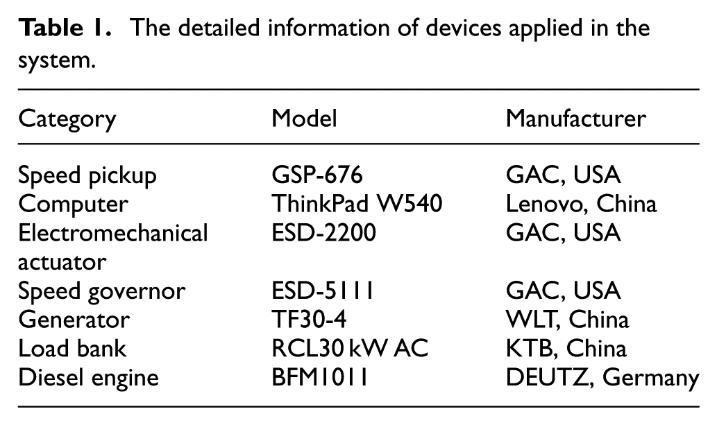
Figure 1 illustrates the structure of this system. The rotational speed of diesel engine, electrical power loads, and rack displacement are required to be collected. Table 1 lists the detailed components of this system. In Figure 1, the actuator is used for driving injector rocker. A displacement sensor embedded in this actuator collects and sends displacement signals to a data acquisition card. There are two speed pickup sensors in this system. One is used to serve for collecting rotational speed signals, which are sent into electronic speed governor. Another is used to serve for data acquisition card. In order to exert and discharge power loads conveniently, a resistive load bank is used in this system. Its purpose is to manually configure different parameters to produce electrical power loads exerted on the DGS. The loading and unloading temporal information and the quantity of electrical power are recorded by a data acquisition card.
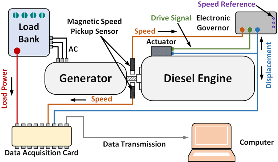
The structure of the DGS system used for collecting data.
The detailed information of devices applied in the system.
Data
In this study, the purpose is to construct a diesel engine model, which is capable of reproducing dynamic characteristics of rotational speed of the DGS with the change of electrical power loads and unloads. To this end, four typical sizes of electrical power values, that is, 7.5, 15, 22.5, and 30 kW, are used for the DGS. Figure 2 shows an experimental data set. In Figure 2, the third figure illustrates that four typical sizes of electrical power values are exerted on one DGS. Depending on different electrical power values, the DGS produces different rack displacements and rotational speeds, which are shown in the first and second figures for Figure 2, respectively. The advantage of selecting those data is that the four typical conditions of the DGS can better reflect the dynamic characteristics of diesel engines.
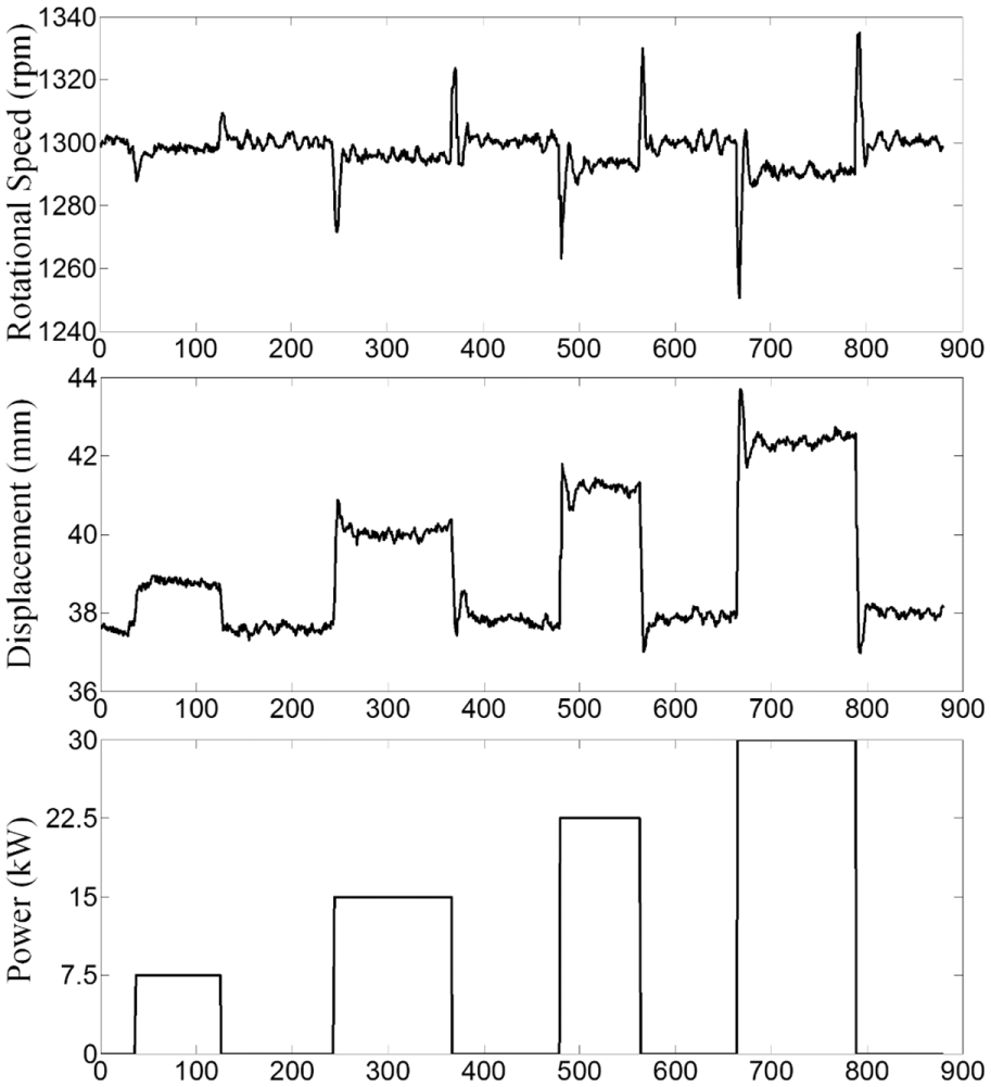
An example set for the rotational speed, rack displacement, and electrical power loads.
A succession of experiments was performed on the condition of 25%, 50%, 75%, and 100% of rated power exerted on the DGS. The rotational speed, loading and unloading power values, and the rack displacement are stored as experimental data. In our study, a total of 2000 experiments were repeated for the experimental data. To be specific, training set has 1400 samples, validation set 300 samples, and testing set 300 samples.
Methods
In this section, the LSTM architecture is first described. Then, the model of diesel engine based on the LSTM is proposed. Finally, the dropout method for the proposed model is given.
LSTM
LSTM is regarded as a special kind of RNN. To better introduce the LSTM theory, we first describe the RNN architecture. The RNN has internal connections between neurons, which form the internal self-looped cell. Its architecture can remember the previous information. In Figure 3, RNN looks like a chain of structures, which are capable of processing longtime sequences. Therefore, RNN has been widely used in learning time series data. 35 The RNN equations can be expressed as follows


where
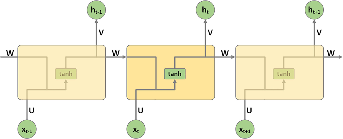
The structure of recurrent neural network.
Generally, RNN is trained through back-propagation through time.36,37 However, the gradient vanishing problem with this method makes the RNN training process not efficient to learn the parameters from long-term dependency. Therefore, the LSTM was proposed for solving this problem. 38 LSTM also has a chain of modules. However, compared with RNN, there are more complicated structures within the LSTM. Each module of LSTM contains a memory block, which can store information over longtime periods. Figure 4 showed a structure of memory block. It mainly consists of four components: three gates, that is, input, forget, and output gates, and constant error carousel (CEC) cell. 39 In the CEC cell, there are no activation functions. It passes through the entire chain. Hence, the back-propagation through time for training a LSTM cannot make the gradient vanishing. Three gates are used to control the information flow in each memory block. To be specific, the input gate controls the input information flows into a CEC cell. The output gate for storing information controls the cell flows into the rest of the LSTM networks.
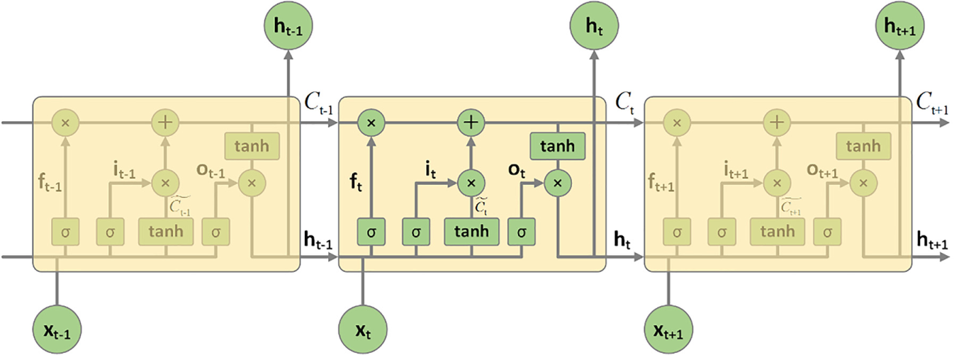
The structure of long short-term memory.
Based on aforementioned description, a mapping can be obtained by the LSTM. Specifically, through computing the network unit activations iteratively, an input sequence


where
The proposed architecture
In term of LSTM architecture, this study proposed an efficient framework for the diesel engine model. As for our work, we are interested in reproducing and predicting the diesel engine’s rotational speed. More specifically, the previous rotational speed has an impact on the current one, that is, the current rotational speed depends on previous one. Consequently, it is regarded as a time series problem. Figure 5 illustrates our proposed regression model. There are two inputs in this architecture. First, the input data are fed into a LSTM layer. In this layer, the input gate recomposes input data and needs to make a decision regarding which input data are significant for the system. The LSTM layer is capable of saving previous information. Hence, this model has a strong ability to learn the data of time series. Then, the outputs of the LSTM layer are sent into a fully connected layer, which is used for predicting the rotational speed of diesel engine. For the fully connected layer in our model, its purpose is to improve fitting ability, since series data cannot be fitted well by an LSTM layer. 40
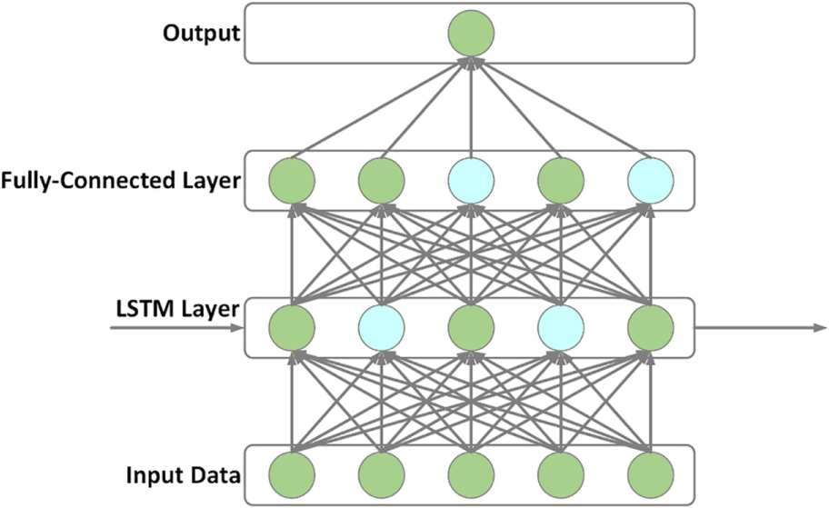
The structure of the proposed model.
In order to limit the overfitting of the model, we added a regularization term into the cost function below
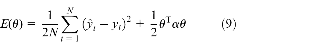
where
In addition, in order to better improve and prevent overfitting, our research adopted the dropout strategy. The detailed information is given in next subsection.
Dropout for LSTM
For deep neural network model, generally, it contains a large number of parameters, which are required to be trained using a lot of data. However, this process can easily produce the overfitting. To solve the overfitting of deep neural networks, the dropout strategy is an effective method.41–43 It can also be regarded as a regularization. In each iteration, it randomly drops out some neurons with probability
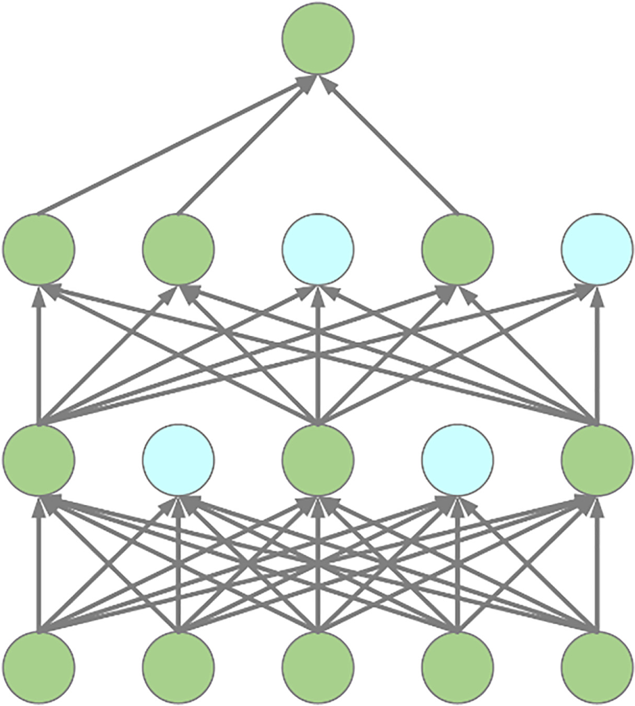
A dropout strategy applied in two hidden layers of neural network: green neurons stand for units in use and light blue neurons stand for dropped units.
Results
The simulation results of the proposed framework are given in this section. First, the evaluation metrics for our method are introduced. Then parameters selection for this model is presented in detail. Third, experimental results under four typical power loading and unloading conditions are reported. Finally, comparison results with other alternative methods are given.
Metrics
Many customary measures are used for evaluating the performance of the LSTM on time series data. 44 For our research, the normalized mean squared error (NMSE), root mean squared error (RMSE), and mean squared error (MSE) are selected as evaluation metrics. The equations of the three metrics can be expressed as follows
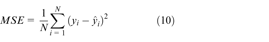
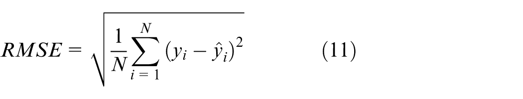
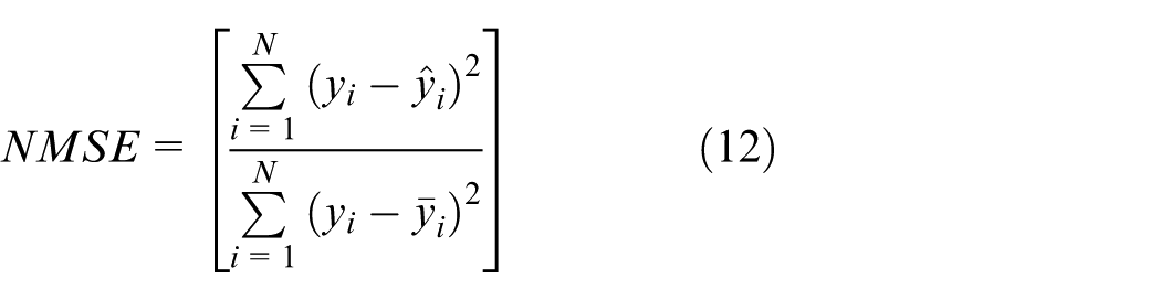
where
Hyper-parameters selection
In the training process, 1400 samples are used for training each chosen LSTM structure, and 300 validation samples for selecting the optimal hyper-parameters including learning rate and the number of neurons of the LSTM. The aim of this process is to select appropriate LSTM structure which is able to meet the desired dynamic behavior of rotational speed for DGS.
Three performance metrics mentioned above are computed to find the optimal hyper-parameters for our proposed model. To achieve this objective, a series of experiments are performed using different combinations with learning rate and the number of hidden neurons. First, we set the variation range of the leaning rate as [10−4, 10−2], and the number of hidden neurons as [10, 60]. To be specific, we first fix the learning rate 10−4. Then, with one interval, the number of hidden neurons is changed from 10 to 60 increasingly. Furthermore, we vary the learning rate increased with 0.0001 interval. The experimental processes are repeated.
Experimental results showed that the output precision of rotational speed was improved with the number of neurons increased. We observed that the metrics of the output decreased a little on the condition of more than 34 neurons. The results showed that the LSTM started to produce data overfitting when it had more than 34 neurons. For the learning rate, we found that the model performance would not be improved when the learning rate was more than 0.0038. Table 2 lists the metrics of the selected LSTM with
Optimized hyper-parameters.
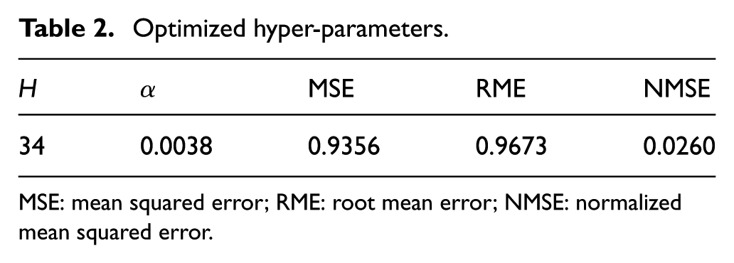
MSE: mean squared error; RME: root mean error; NMSE: normalized mean squared error.
Experimental results
Using the best LSTM structure, this section gives the experimental results performed on the testing data. The aim of our research is to reproduce the dynamic characteristics of diesel engine under four types of representative electrical power loads including 7.5, 15, 22.5, and 30 kW. According to subsection “Setup,” the experimental data consist of four dynamic characteristics with different electrical power loads. Here, we divide the data into four segments with each one containing 20-s data. Specifically, in the beginning phase, the electrical power would be exerted on the proposed model of diesel engine, and then discharged from it. The whole process should be finished within 20-s period.
To illustrate the performance, Figure 7 shows the predicted rotational speed curves produced by the LSTM and measured data on the conditions of 7.5, 15, 22.5, and 30-kW loads, respectively. We observed that the predicted rotational speed was in good with measured data. Table 3 lists the three metric results performed on the testing data. Results showed that the best prediction error was occurred under the 30-kW load. Generally, the performance of diesel engine with the full power load is a very important factor for developing the electronic speed governor.
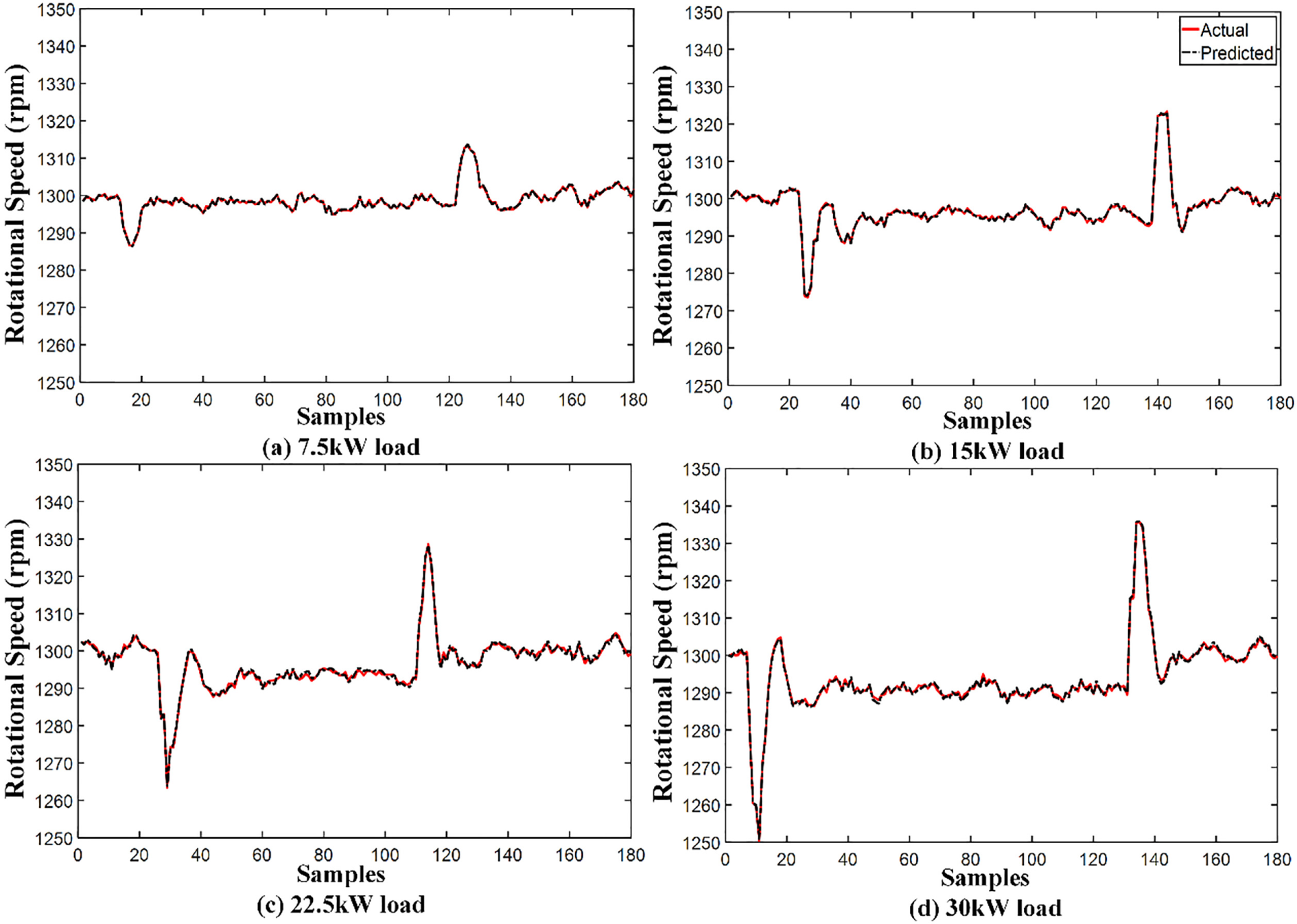
Actual and predicted rotational speed of the diesel engine model with: (a) 7.5, (b) 15, (c) 22.5, and (d) 30 kW.
Results performed under 7.5, 15, 22.5, and 30 kW.
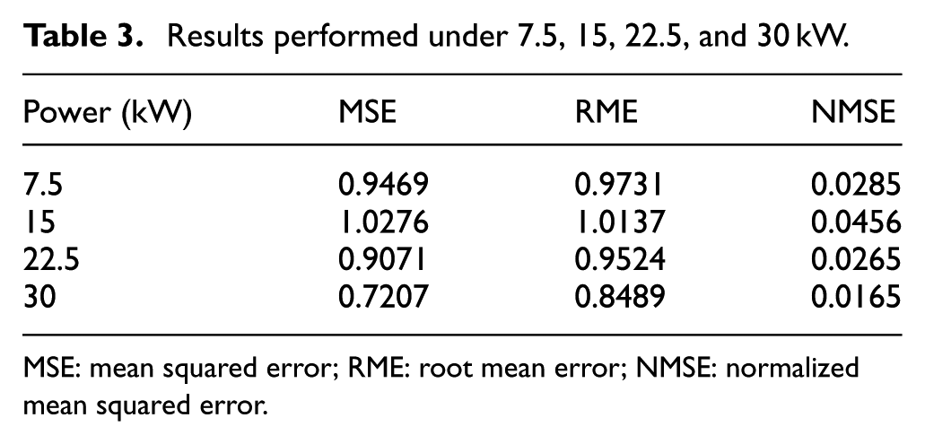
MSE: mean squared error; RME: root mean error; NMSE: normalized mean squared error.
Comparison with other approaches
To show the advantages of our proposed LSTM framework, we report the performance comparison with other approaches, that is, polynomial NARX, NARX RNN, and multi-layer perception feed forward (MLPFF) neural network. All have been applied in prediction task for time series data. Considering the sake of fairness, all of approaches are performed on our established dataset and with the same performance metrics. In our research, the rotational speed of DGS is required to be reproduced on the condition of changing electrical power loads. Table 4 lists the comparison results using MSE, root mean error (RME), and NMSE metrics under 7.5, 15, 22.5, and 30-kW loads, respectively. Table 4 shows our method obtains best prediction performance in MSE, RME, and NMSE.
Comparison with other methods under four types of power loads, that is, 7.5, 15, 22.5, and 30 kW.
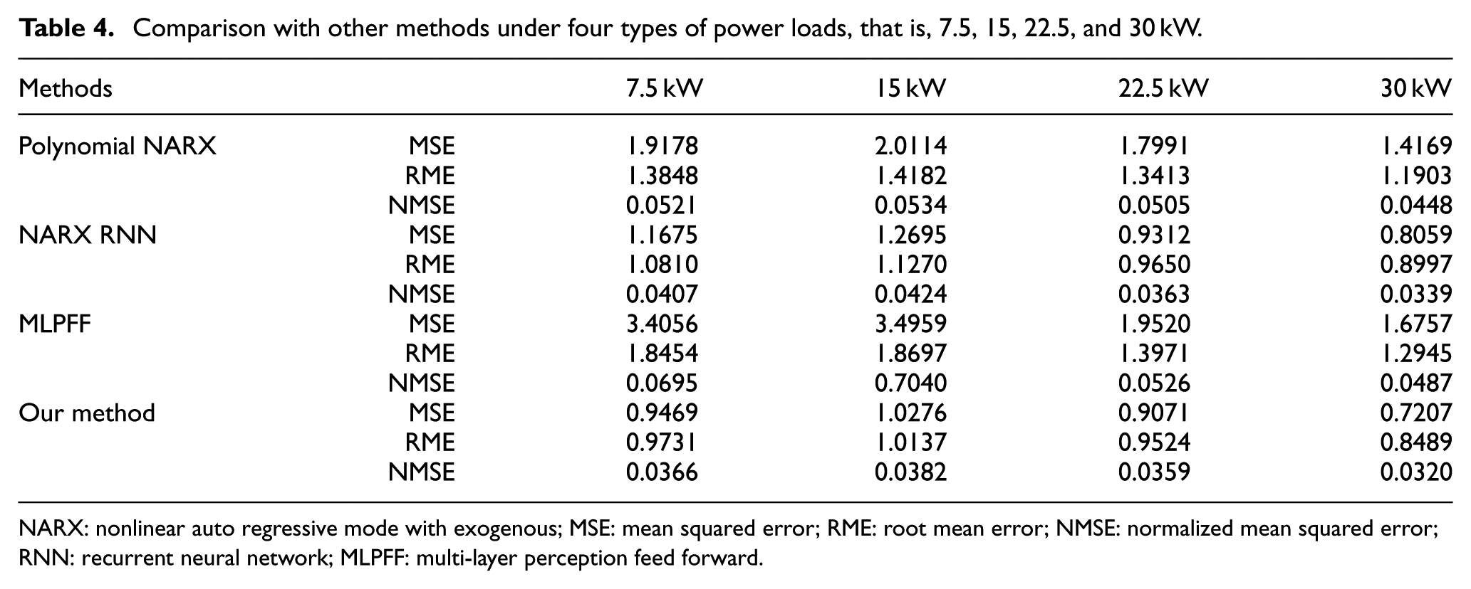
NARX: nonlinear auto regressive mode with exogenous; MSE: mean squared error; RME: root mean error; NMSE: normalized mean squared error; RNN: recurrent neural network; MLPFF: multi-layer perception feed forward.
HIL simulation system
First, the HIL for the DGS is established by us. Then, the performance metrics for this system is proposed under power loading and unloading conditions.
HIL setup
Figure 8 shows the structure of the DGS HIL simulation system. It consists of software and physical objects. The software represented by the optimized models is run on the host PC to simulate the rotational speed of DGS. The physical objects contain electronic actuator, signal conditioning board, data acquisition card, electronic governor, speed pickup, and three-phase AC servomotor. The rotational speed of DGS is simulated by the AC servomotor.
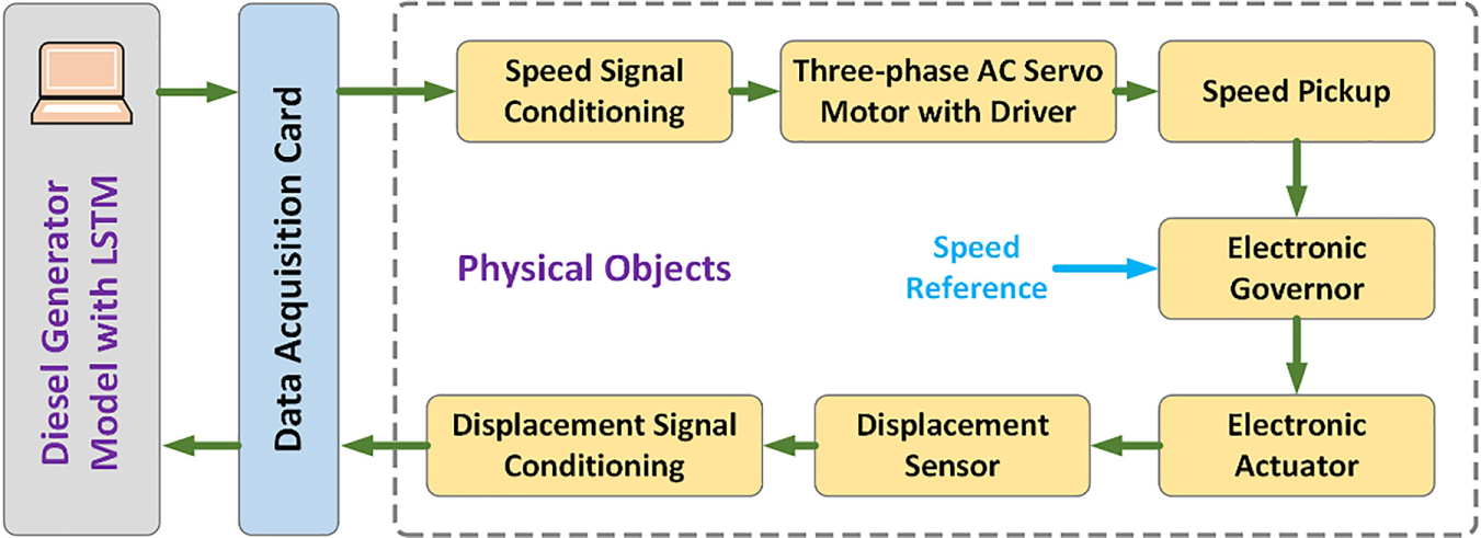
The HIL simulation system of diesel generator sets.
The operation process of the HIL simulation system can be described as follows. First, the speed pickup installed in an AC servomotor captures its rotational speed signal. Then, it is sent into an electronic speed governor. In our work, the rotational speed is set as 1300 r/min. The actuator for controlling the rack displacement of the engine fuel is driven by an electronic speed governor. The displacement can be measured by a sensor embedded in the actuator. Furthermore, this signal is fed into the conditioning board and sent into the host PC. With the rack displacement, the proposed DGS model is able to compute and simulate the rotational speed. Finally, the speed signal is feedbacked into the AC servomotor. The whole process can be regarded as a closed system to simulate the dynamic characteristics of the DGS. Thus, the electronic speed governor which severed for a DGS can be developed and debugged on this system.
Evaluation
The transient regulation ratio (TRR) and the settling time (ST) are used as two metrics for evaluating the performance of the HIL simulation system, as follows 27


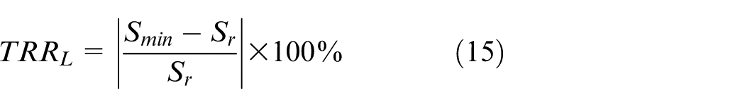
where
For this simulation, we chose the ESD-2200 of GAC as the electronic speed governor. The reference speed is assigned at 1300 r/min. The simulation evaluation of rotational speed needs to meet the following criteria 27 : the TRR is not more than 5%, and the ST less than 3 s. The loading and unloading power values are manually controlled by a power load bank.
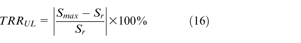
Using equations (13)–(16), the performance measures are shown in Table 5. In Figure 9, simulation results showed that the proposed diesel model successfully reproduces the dynamic processes under 7.5, 15, 22.5, and 30-kW loading and unloading conditions, respectively. From Figure 9, the important challenging index for loading and unloading conditions is 30 kW in our HIL system. To be specific, the HIL system obtained 1.7 s of ST and 3.61% of TRR when the power exerted on the diesel model, 1.7 s of ST and 3.47% of TRR when the power discharged from the diesel model. All of results obtained from the HIL system meet the requirements. Therefore, the HIL with our proposed model can be used in debugging and developing the electronic speed governor of on-board condition. The software run in host PC was programmed by the LabVIEW 2013.
Evaluation results obtained from the HIL simulation system.
HIL: hardware-in-the-loop.
The speed curves obtained by the HIL simulation system with different power loads: (a) 7.5, (b) 15, (c) 22.5, and (d) 30 kW.
Conclusion
Using the LSTM neural network theory, this study proposed a novel diesel engine model. It can successfully reproduce and simulate the rotational speed of DGS under different power loading and unloading conditions. Compared with existing methods, the results obtained provide an evidence that the performance of our model outperforms others. Furthermore, this model is deployed on an established HIL simulation system. The results show that our proposed model is able to reproduce well the dynamic characteristics of the DGS on the condition of exerting power loads on the DGS and discharging from it. Consequently, the HIL simulation system can be regarded as a real environment to develop and debug the electronic speed governor.
Footnotes
Acknowledgements
We thank all the reviewers who gave the valuable suggestions for improving this study.
Declaration of conflicting interests
The author(s) declared no potential conflicts of interest with respect to the research, authorship, and/or publication of this article.
Funding
The author(s) received no financial support for the research, authorship, and/or publication of this article.