
Abstract
Methods for the accurate prediction of icing loads in overhead transmission lines have become an important research topic for electrical power systems as they are necessary for ensuring the safety and stability of power-grid operations. Current machine learning models for the prediction of icing loads on transmission lines are afflicted by the following issues: insufficient prediction accuracy, high randomity in the selection of kernel functions and model parameters, and a lack of generalizability. To address these issues, we propose a field data–driven online prediction model for icing loads on transmission lines. First, the effects of the type of kernel function used in the support vector regression algorithm on the prediction accuracy of the model were analyzed using micrometeorological data and icing data collected by on-site monitoring systems. The particle swarm optimization algorithm was then used to optimize and determine the model parameters such as penalty coefficients. An offline support vector regression prediction model was thus constructed. Using the accurate online support vector regression algorithm, the weighting coefficients of the samples were dynamically adjusted to satisfy the Karush–Kuhn–Tucker conditions, which allowed online updates to be made to the regression function and prediction model. Finally, a simulation analysis was performed using actual icing incidents that occurred in a transmission line of the Yunnan Power Grid, which demonstrated that our model can make online predictions for the icing load on transmission lines in actual applications. Our model proved to be superior to conventional icing-load prediction models with regard to the single-step and multi-step prediction accuracies and generalizability. Hence, our prediction model will improve the decision-making processes regarding the deicing and maintenance of power transmission and transformation systems.
Introduction
The reliability, maintainability, and safety of power facilities such as power stations and power grids are important for the security of national economies and the livelihoods of people.1–3 However, the overhead power transmission line icing disaster caused by a variety of extreme weather phenomena has resulted in great damage to transmission lines and equipment in most countries.4–7 Owing to the effects of global warming, the frequency of extreme weather incidents has gradually increased over the past few years. Consequently, severe weather-induced icing incidents are among the most important sources of risk in power-grid operations. A field data–driven online icing-load prediction model that provides prediction-based early warnings can guide the decision-making processes regarding the maintenance and deicing of power transformation and transmission systems, thus alleviating losses in power grids caused by the icing of transmission lines. Hence, the creation of such a model is an important and urgent task for this field of research. Thus far, numerous studies have been performed on the ice accretion on transmission lines by researchers around the world, yielding many significant achievements. The results of these studies can be generally categorized as mechanistic models, statistical models, and machine learning models:
Mechanistic models:8–11 Marcacci et al. 8 conducted a computational analysis of the effects of air temperature, wind speed, and droplet diameter on the icing intensity and local collision rates during icing processes. On this basis, a computational module for computing ice accretion on transmission lines was developed, and the icing processes were numerically simulated. A model for predicting the equivalent ice-accretion thickness of the combined load on overhead transmission lines was proposed in Jiang et al., 9 based on the static force balance theory. Yan et al. 10 proposed a method for carrying out short-term icing predictions to determine the risk of icing hazards in power grids. Jiang et al. 11 analyzed the changes in the mechanics of a wire after ice accretion with respect to the axial tension and angle of inclination of the line. On this basis, an accurate model for predicting the icing of a single wire was constructed, and a manual method for on-site measurements of the equivalent ice thickness of a wire was proposed.
Statistical models:12–16 Wang et al. 12 performed statistical analyses of the icing of transmission lines using data from an online monitoring system. The trends in the development of ice accretion on transmission lines were investigated through collection of icing data pertaining to short-term oscillations, medium- to short-term trends, and long-term trends. Jiazheng et al. 13 calculated the recurrence interval of severe grid icing incidents using a Type I extreme value distribution for the ice-accretion thicknesses and a system for grading the severity of icing incidents, according to observational data from icing incidents that occurred in the Hunan Province. Wang et al. 14 analyzed the factors that influence the suitability of extreme value estimation models in estimating ice-accretion values, along with the suitability of each extreme value distribution for different icing regions. In addition, various sampling methods were used to estimate the recurrence interval of extreme ice-accretion thicknesses.
Machine learning models:17–24 Liu et al. 17 used a multivariate gray model to predict the short-term ice-accretion thicknesses. To reduce the effects of cumulative errors from various micrometeorological factors on icing predictions, a model for predicting short-term icing on transmission lines was proposed in Huang et al., 18 based on a mixture of time-series analysis and the Kalman filter algorithm. In the study by Dai et al., 19 the parameters most strongly correlated with transmission line icing, that is, air temperature, air humidity, and reference icing data were used as input data, and the icing mass was used as the output data. On this basis, three different support vector regression (SVR)-based models were proposed: a super short-term forecast model, a short-term hysteresis forecast model, and a rolling forecast model.
Generally, mechanical and statistical models for the prediction of icing loads are based on analytical models. However, owing to the large number of factors that ultimately determine the icing load of a transmission line and the fact that icing processes are highly dimensional non-linear processes, it is very difficult to construct analytical models for this process. Therefore, the generalization of a transmission line icing model to other transmission lines is usually very difficult, especially if there are significant differences between the geographical environments of the transmission lines. Li et al. 25 provided a field data–driven prediction model but did not consider the time-series problem and generalizability of backpropagation neural network (BPNN). Hence, there are significant problems in the robustness of current icing-prediction models. On the contrary, machine learning–based icing-prediction models can effectively predict the icing loads of a transmission line using historical field data. However, these models lack prediction accuracy, have high levels of randomity in the selection of kernel functions and model parameters, are not easily generalizable, and are strongly reliant on historical sample data. For example, as extreme icing disasters are low-probability events, it is difficult to obtain sample data on icing disasters that occur once every few decades or every hundred years. Thus, conventional machine learning models that rely heavily on the comprehensiveness of their training sets are ineffective for these rare events.
In this study, time-series analyses of the icing processes of transmission lines were performed. The effects of the kernel function type on the prediction accuracies of the prediction models were analyzed, and the particle swarm optimization (PSO) algorithm was used to optimize all the model parameters. Finally, a field data–driven online prediction model for the icing loads on transmission lines was proposed by combining offline modeling with online updating methods, according to the concept of data-driven modeling. To validate the effectiveness of our model, a quantitative analysis of the icing processes was performed at the Tao-Luo-Xiong line of the Yunnan Power Grid in northeastern Yunnan, using actual ice monitoring data from the transmission line. For more intuitive performance, BPNN, SVR, least square support vector regression (LS-SVR), and extreme learning machine (ELM) optimized by several optimization algorithm are chosen as comparisons. This comparison included the single-step and multi-step prediction accuracies, generalizability, execution efficiency, and ability to approximate the target mapping. An innovate hybrid model is successfully proposed for multi-step-ahead icing-load prediction of the power transmission lines and to design numerical experiments from the real icing power transmission lines to validate the availability and reliability of the developed model. The results of this experiment demonstrate that our model is capable of mining historical icing data and micrometeorological data, constructing mapping relations between micrometeorological data and icing processes, and dynamically updating itself using real-time micrometeorological data extracted from online ice monitoring systems. This makes it possible to accurately model local icing loads on transmission lines. In addition, the practical engineering significance of our model has been proven by the general consistency between its predictions and actual icing-load data.
The rest of the paper is organized as follows. Section “Time-series analyses of icing on transmission lines” describes the time-series analyses of icing on transmission lines. Section “Principles of accurate online support vector regression” details the principles of accurate online SVR. In section “Online prediction model for icing loads on transmission lines,” an online prediction model is presented for icing load on transmission lines and the model is constructed and detailed. Numerical tests are performed and discussed in section “Simulation analysis.” The conclusions are summarized in section “Conclusion.”
Time-series analyses of icing on transmission lines
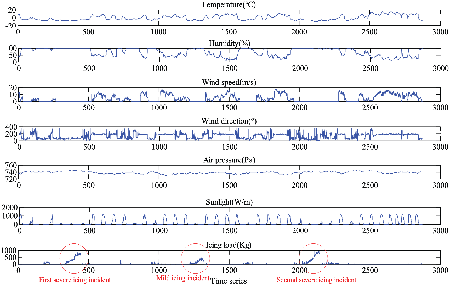
Ice accretion on transmission lines occurs under certain weather conditions, and both micrometeorological and wire-related factors can affect the development of icing loads on transmission lines. The online monitoring of ice accretion on transmission lines is generally performed through the installation of mechanical and weather sensors in sites where icing occurs on transmission lines, which allows for the acquisition of icing-load data and the corresponding micrometeorological data. Curve fitting may then be performed to identify trends in the icing-load data. The on-site micrometeorological data and icing-load data shown in Figure 1 correspond to the intermittent icing of the Tao-Luo-Xiong line in northeastern Yunnan, from 14 December 2009 to 25 January 2010, and the ice accretion is sampled in 20-min intervals (Δt = 20 min). The sampling period of icing dataset is 42 days. According to the icing load, we divide the data into three parts: first severe icing incident, mild icing incident, and second severe icing incident.
Intermittent icing of the Tao-Luo-Xiong line.
Figure 1 shows that the icing load on the transmission line increases rapidly over the duration of an icing incident. This is especially apparent during extended periods of freezing rain; in these cases, it only takes 1–2 days for the icing load of the transmission line to reach the designed icing load of the transmission tower. Therefore, the creation of a time-effective method for analyzing the effects of micrometeorological effects on icing processes is an urgent task in this field of research.
Equation (1) presents the thermodynamic mechanism of ice accretion in the Makkonen model 26
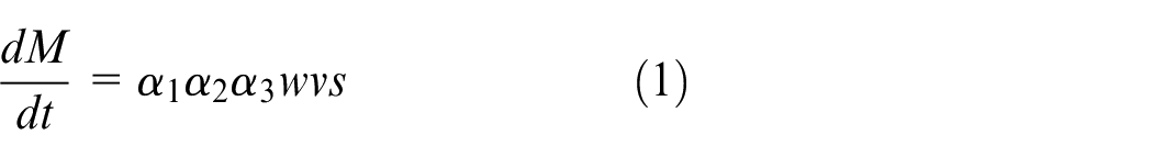
where
The discrete-state equation for icing processes on transmission lines can be derived from the thermodynamic mechanisms of accreted ice growth, as follows
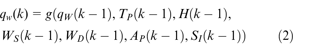
where g(*) is the mapping between the icing load of the transmission line and the micrometeorological factors; qw is the unit icing load of the transmission line; Tp and H are environmental temperature and humidity, respectively; WS and WD are the wind speed and wind direction, respectively; AP is the ambient pressure; SI is the solar irradiance; and k is the sampling time.
Equation (2) indicates that the icing load of a transmission line at time k is determined by micrometeorological factors and also the icing load at time k – 1. Because the mapping between the micrometeorological factors and the icing load, g(*), is non-linear and depends on the micro-meteorology and micro-topography of the monitoring point, this equation is a multivariate time series.
Principles of accurate online support vector regression
Principles of discrete SVR and optimization of its parameters
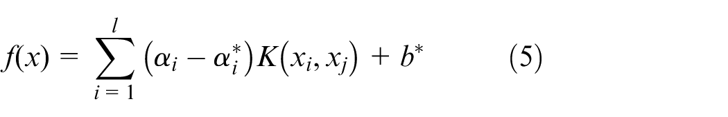
SVR is based on the principles of structural risk minimization: if there is a non-linear mapping, Φ(x), that maps the input dataset to a high-dimensional feature space, F, there is a linear function f(x) in this space that clearly defines the non-linear relationship between the input and output datasets. The definitions of the functions in SVR are as follows.27,28
Given a training set

where
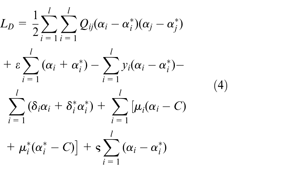
where C is the penalty coefficient, ε is the insensitive loss coefficient, and
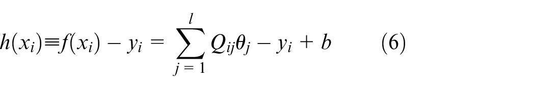
A boundary function is defined for sample
The penalty coefficient C plays a crucial role in the complexity and stability of the model, whereas the insensitive loss coefficient ε determines the width of the insensitive region used to fit the regression function to the sample data. Thus, to construct an accurate SVR model, it is necessary to optimize C, ε, and all the other parameters of the kernel function.
PSO, which was proposed by Kennedy and Eberhart, is an optimization algorithm based on swarm intelligence.29,30 By comparing the accuracy and efficiency of genetic algorithm (GA), PSO represents the closer convergence solution to the global optimum and quicker convergence to the solution, especially the improvement of best fitting value.31,32 In this algorithm, the search for global optima is achieved via cooperation and competition between individuals. The principles of this algorithm are as follows: suppose that there is a population comprising m particles in an n-dimensional search space, such that
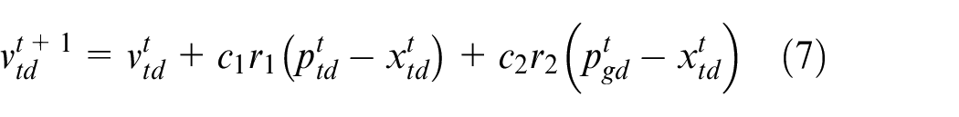

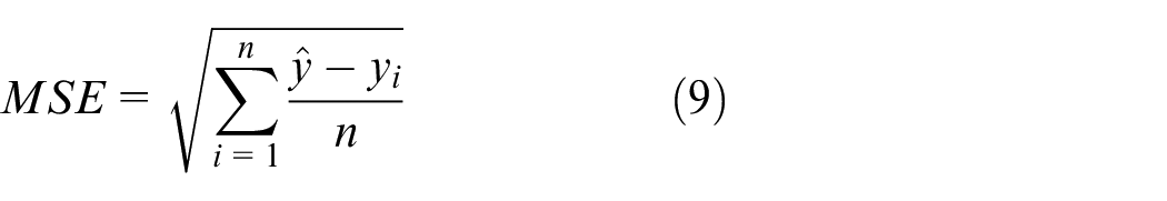
where d = 1, 2, and n, while i = 1, 2, and m; m is the size of the population, t is the current evolutional generation, r1 and r2 are random numbers in the interval of [0, 1], and c1 and c2 are acceleration constants. The fitness function is the mean square error (MSE) (equation (9)), which reflects the regression performance of the SVR model
where
Online SVR and Karush–Kuhn–Tucker conditions
Online SVR is a type of regression modeling method that allows for the updating of prediction models in an online, dynamic fashion. Ma et al. proposed the accurate online support vector regression (AOSVR) incremental learning algorithm based on online SVR algorithms.
33
The core idea of the AOSVR algorithm is to update all the difference coefficients (θc) corresponding to any newly added sample
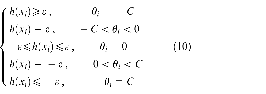
When the optimal solution to this problem is found, the samples can be divided into the following three classes according to the KKT conditions and Lagrangian multiplier method:
Error support vectors:
Margin support vectors:
Remaining samples:
The procedures of the AOSVR algorithm are as follows. Define the new samples as
If the sample index of the support vector is defined as
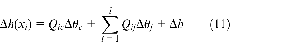
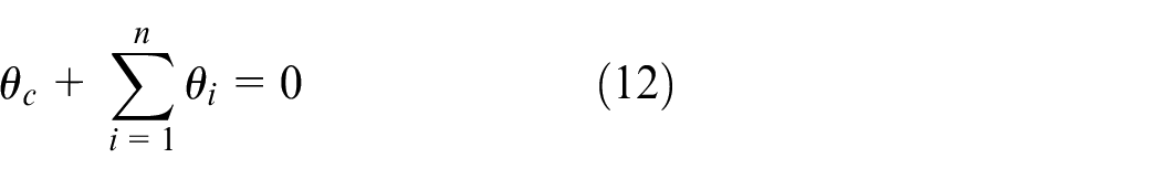
Combining equations (10) and (11), equation (12) can be expressed in matrix form as
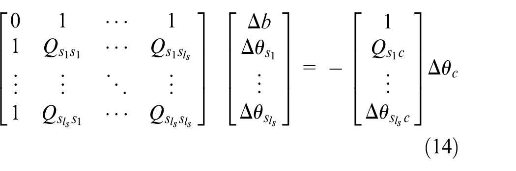
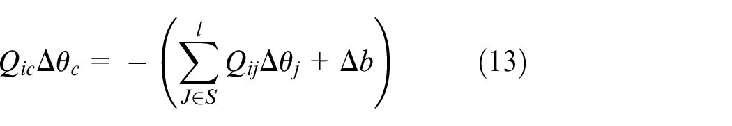
Equation (13) can be represented in another form as
Here

Define
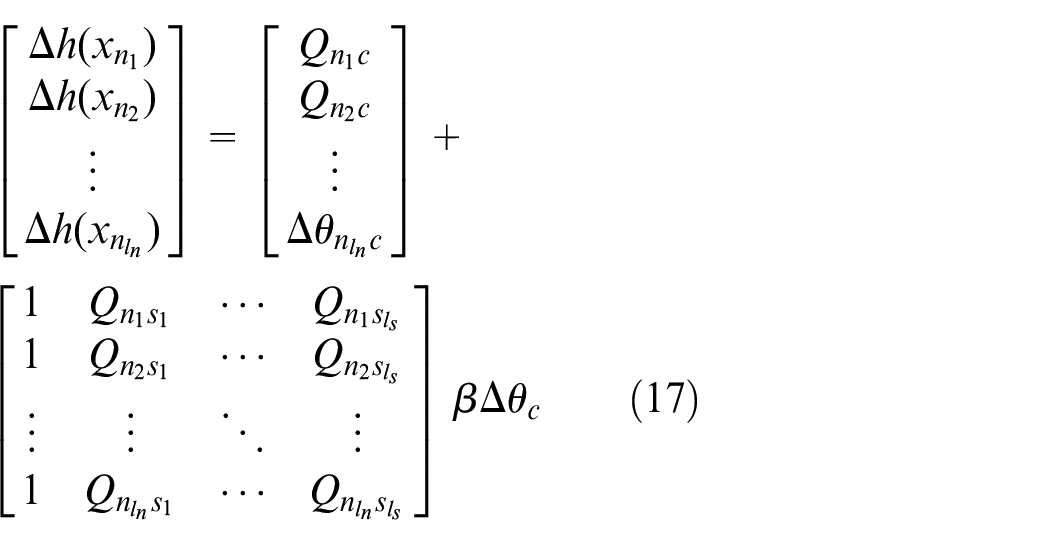
By incremental learning in the AOSVR algorithm and the updating of the S, E, and R sample sets, we can update
Online prediction model for icing loads on transmission lines
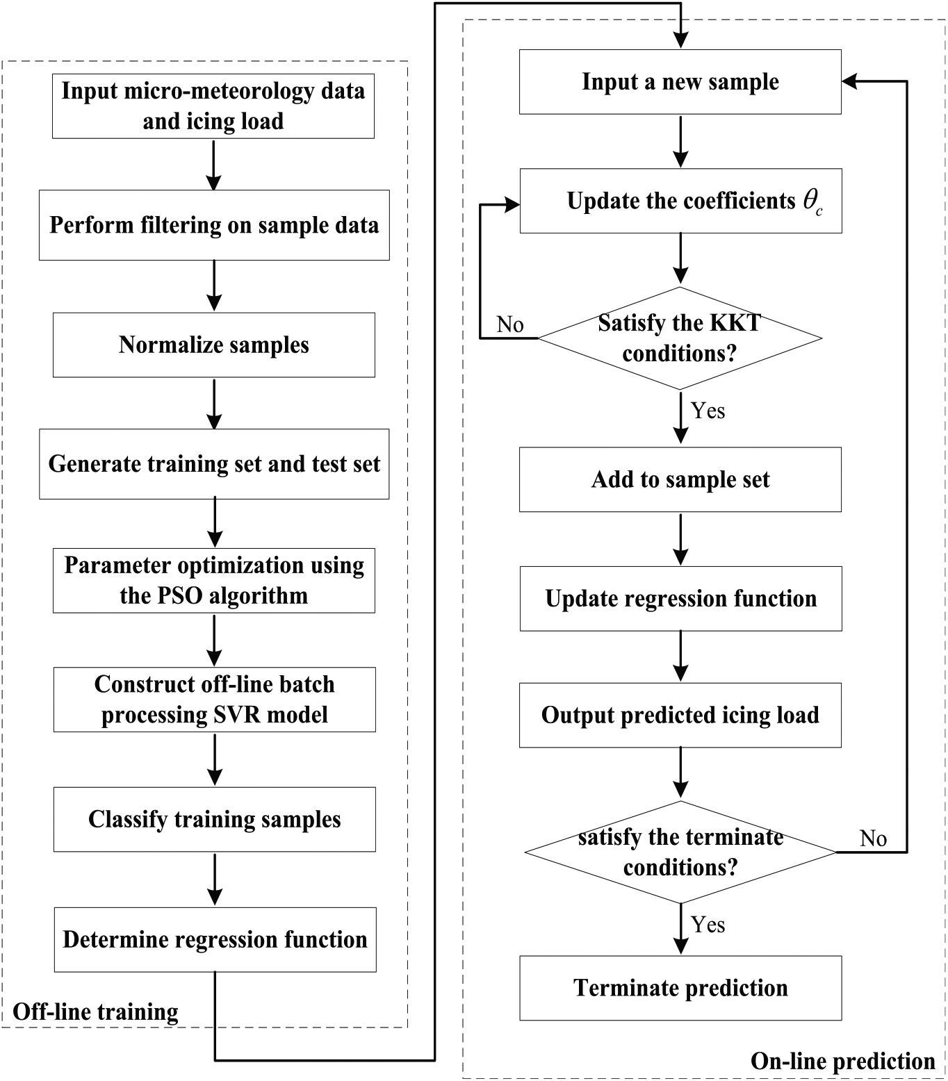
The basic idea underlying the construction of our prediction model for icing loads on transmission lines is the definition of a non-linear mapping Φ(x) that maps micrometeorological data to a high-dimensional feature space, followed by the linear regression of icing loads in this feature space. The field data–driven online prediction model for icing loads on transmission lines constructed in this work is shown in Figure 2. This model can be divided into three parts:
Data preprocessing;
Training of the offline SVR model;
Online updating of the SVR model and icing-load prediction.
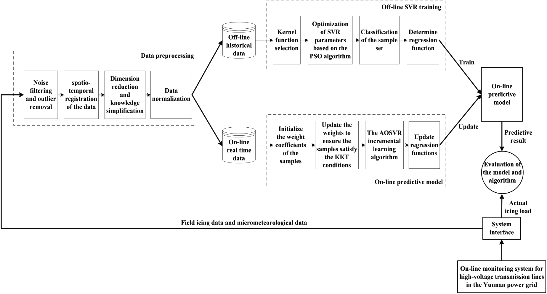
Field data–driven online prediction model for the icing load on transmission lines.
Data preprocessing
The following data preprocessing steps were performed on the sample set to reduce the impact of outlying data points on the regression performance and to increase the training speed of the model.
Sample filtering, de-noising, and dimension reduction
Wavelet analysis, weighted moving average filtering, and particle filtering algorithms were used to perform de-noising, outlier removal, and spatiotemporal registration on the offline historical data (icing load and meteorological information). Principal component analysis and rough set algorithms were then used to perform dimension reduction and knowledge simplification on the multi-dimensional data, such as icing loads and meteorological information.
Outlier data were removed from the measurement data according to the following requirements for ice accretion in overhead transmission lines: air temperature and equipment surface temperatures of 0 °C or lower, and a relative air humidity of 80% or higher.
Data normalization
Min–max normalization was used to normalize the sample set
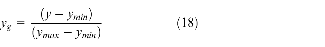
where yg is the normalized data, y is the original data in the sample set, and ymin and ymax are the minimum and maximum values of y, respectively.
Training of offline SVR model
To construct an offline SVR training model, the type of the kernel function and the model parameters must be determined beforehand. In this study, four common kernel functions were used to independently construct four different training models. The best kernel function was selected, and the PSO algorithm was then used to optimize the relevant parameters. The detailed steps of this procedure are as follows.
Step 1: Select a suitable training sample set for the model. The first severe icing incident (Figure 1) was chosen as the training sample set when the regression performance of the model was examined, whereas a mild icing incident was used as the training set when the generalizability of the model was examined. Micrometeorological data (including temperature, humidity, wind speed, wind direction, pressure, and solar irradiance) were used as the inputs of the model, and the icing load was the output.
Step 2: Select the type of kernel function. The linear kernel function, RBF kernel function, polynomial kernel function, and sigmoid kernel function were independently used to construct training models. The icing-prediction models based on these kernel functions were then compared with regard to their single-step and multi-step regression performances, and the kernel function yielding the smallest error was used to train the offline SVR model.
Step 3: Optimize regression parameters using the PSO algorithm. To improve the regression accuracy of the prediction model, the PSO algorithm was used to optimize the parameters of the penalty coefficient (C), insensitive loss coefficient (ε), and all other parameters of the kernel function.
Step 4: Classify the training set. The training sample set was divided according to the KKT conditions into error support vectors (E), margin support vectors (S), and remaining samples (R).
Step 5: Determine the regression function. The offline batch-processed SVR model was constructed according to the training set, yielding the regression function of the model, f(x).
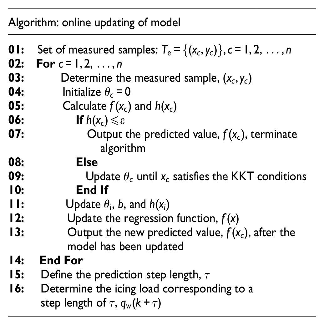
Online updating of model and icing-load predictions
Conventional prediction models for icing on transmission lines based on the BPNN and SVR algorithms cannot be dynamically updated upon the addition of new measurement samples, reducing their prediction accuracy. The field data–driven online prediction model proposed herein is based on the incorporation of the AOSVR algorithm into current offline SVR models. In our model, the weighting coefficients of the samples are dynamically adjusted to ensure that they satisfy the KKT conditions, allowing the regression function and prediction model to be updated online. The algorithmic procedure of our model is shown in Figure 3.
Flowchart of the online model for predicting icing loads on transmission lines.
Figure 3 shows that the samples are processed one by one as they are added to the model. According to the regression function and weighting coefficients (θi) obtained from the training set—and by assuming a weighting coefficient of 0—the newly added measurement data are assessed to determine whether they satisfy the KKT conditions. After a new regression function is obtained by dynamically adjusting the weighting coefficients according to the newly added sample, the prediction model is updated, while its fitness with respect to the test samples is optimized. This procedure allows a regression model to be modified online, improving the ability of the model to approximate the target mapping and its accuracy in icing-load predictions. Therefore, the proposed field data–driven online prediction model can perform adaptive and dynamic modeling.
To examine the regression performance and generalizability of our models, single-step and multi-step predictions were performed on the samples that were measured during the second severe icing incident (Figure 1). A single-step prediction refers to the prediction of the icing load (K = 1) at time n, based on the micrometeorological information corresponding to all times up to n – 1.
The pseudocode for performing online updates in our model and for multi-step icing-load predictions is shown below.
Simulation analysis
The several experiments listed below were used to evaluate our field data–driven online prediction model for the icing loads on transmission lines:
Optimization of regression parameters using PSO algorithm;
Selection of optimal kernel function;
Comparison between our model and other four models in single-step and multi-step predictions;
Comparison between our model and other four models with regard to generalizability and efficiency.
Evaluation indices
The data used in this experiment are the 2872 data points corresponding to the intermittent ice-accretion processes on the Tao-Luo-Xiong line in northeastern Yunnan, from the end of 2009 to the beginning of 2010 (see Figure 1). These data were acquired with a sampling interval of Δt = 20 min. To evaluate the predictive capabilities of the models, the data corresponding to the first severe icing incident (17–20 December 2009) were used as the training set for constructing prediction models; these models were then used to predict the second severe icing incident (10–12 January 2010). When the generalizability of the models was examined, the test set was kept unchanged, and the data corresponding to the mild icing incident (30 December 2009 to 2 January 2010) were used as the training set.
The following three indices were used to evaluate the regression performance of the models:
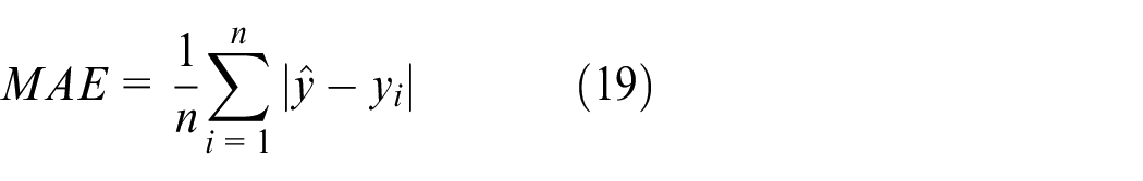
Mean absolute error (MAE)
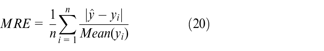
Mean relative error (MRE)
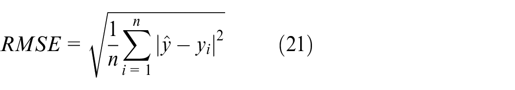
Root-mean-square error (RMSE)
where
Results of parameter optimization using PSO algorithm
The penalty coefficient (C), insensitive loss coefficient (ε), and other kernel function parameters form the solution space that determines the position and velocity of each particle. The parameters of the particles were initialized as follows: population size m = 10, acceleration coefficients a1 = a2 = 2, C in the interval of [0, 50], ε in the interval of [0, 1], and maximum evolutional generation of Tmax = 200. The 220 data points corresponding to the first severe icing incident were used as the training set. The results of the PSO parameter optimization are shown in Table 1.
Results of particle swarm optimization optimization for the regression parameters of different kernel functions.
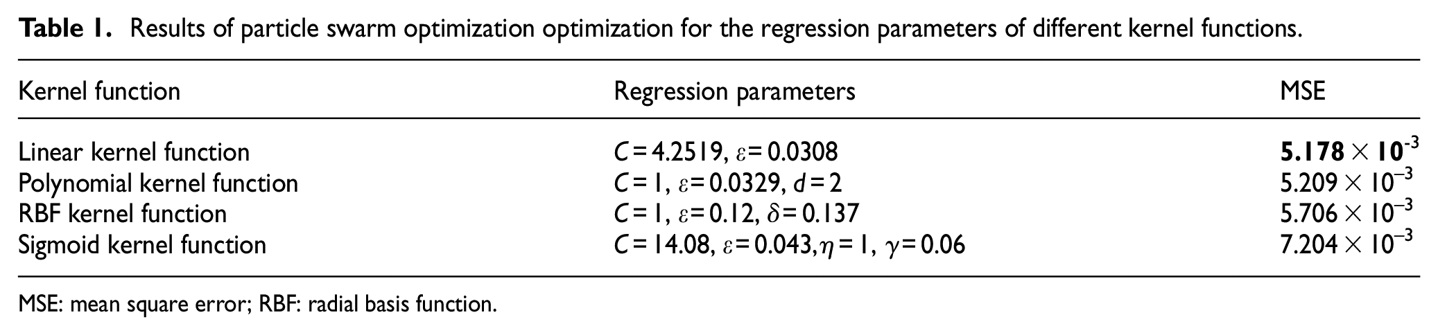
MSE: mean square error; RBF: radial basis function.
Comparison of multi-step prediction accuracy among four different kernel functions
Four models using the linear, RBF, polynomial, and sigmoid kernel functions were trained using the 220 samples of the first severe icing incident. These models were then used to perform single-step and multi-step predictions on 139 samples corresponding to the icing load on the Tao-Luo-Xiong transmission line during the second severe icing incident, and the ice accretion is sampled in 20-min intervals (Δt = 20 min). The MAE, MRE, and RMSE of each model were calculated using equations (16), (17), and (18), respectively, and the results are shown in Figure 4.
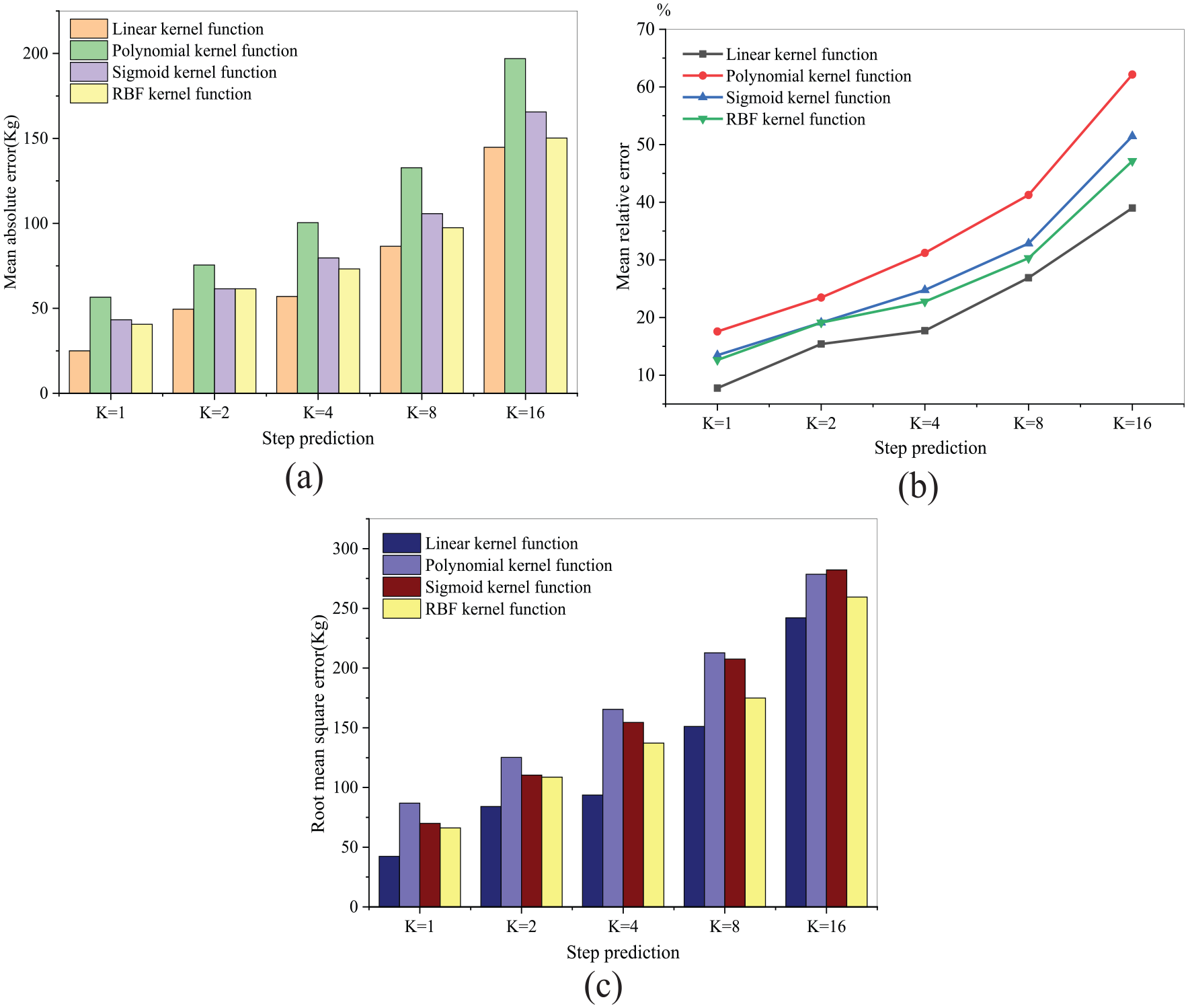
Comparison of the accuracy among four different kernel functions: (a) MAE, (b) MRE, and (c) RMSE.
Figure 4 shows that the MAE, MRE, and RMSE of the kernel functions increase at different rates with increases in the step length. This comparative experiment indicates that the linear kernel function in our online icing-load prediction model yields the highest single-step and multi-step prediction accuracies.
Comparison between single-step and multi-step predictions of five different models
The effectiveness and scientific accuracy of our model for the prediction of icing loads on transmission lines were validated through comparisons with conventional BPNN- and SVR-based icing load models, with regard to the ability of the models to approximate the target mapping and the accuracy of their single-step and multi-step predictions. Parameters used in BPNN were optimized through tracking error analysis, and the node number of the hidden layer is 80. The transfer function from the input layer to the hidden layer is tansig and from the hidden layer to the output layer is logsig. Parameters for the standard SVR were optimized by PSO, the kernel function is RBF kernel function, the penalty coefficient C = 4, the insensitive loss coefficient is 0.01, and the parameter of RBF kernel function δ = 0.267. Parameters used in LS-SVR were optimized by PSO, the kernel function is linear kernel function, the penalty coefficient C = 11.838, and the insensitive loss coefficient is 100. Parameters for ELM were optimized by cross-validation, the node number of the hidden layer is 13, and the activation function is sigmoid function. Parameters for our model were optimized according to Table 1; the kernel functions is linear kernel function, the penalty coefficient C = 4.2519, and the insensitive loss coefficient ε = 0.0308.
An objective comparison was performed between the regression accuracies of these icing-prediction models by using the same validation data for each prediction model. The time-series curves for the first and second severe icing incidents shown in Figure 5(a) were used as the training and test set output of the regression models, respectively, and it is shown that the greatest icing loads during these events are 814.5 and 951.9 kg, respectively. The results of the single-step ice-accretion predictions are shown in Figure 5, and the results of the multi-step predictions are shown in Tables 2–4.
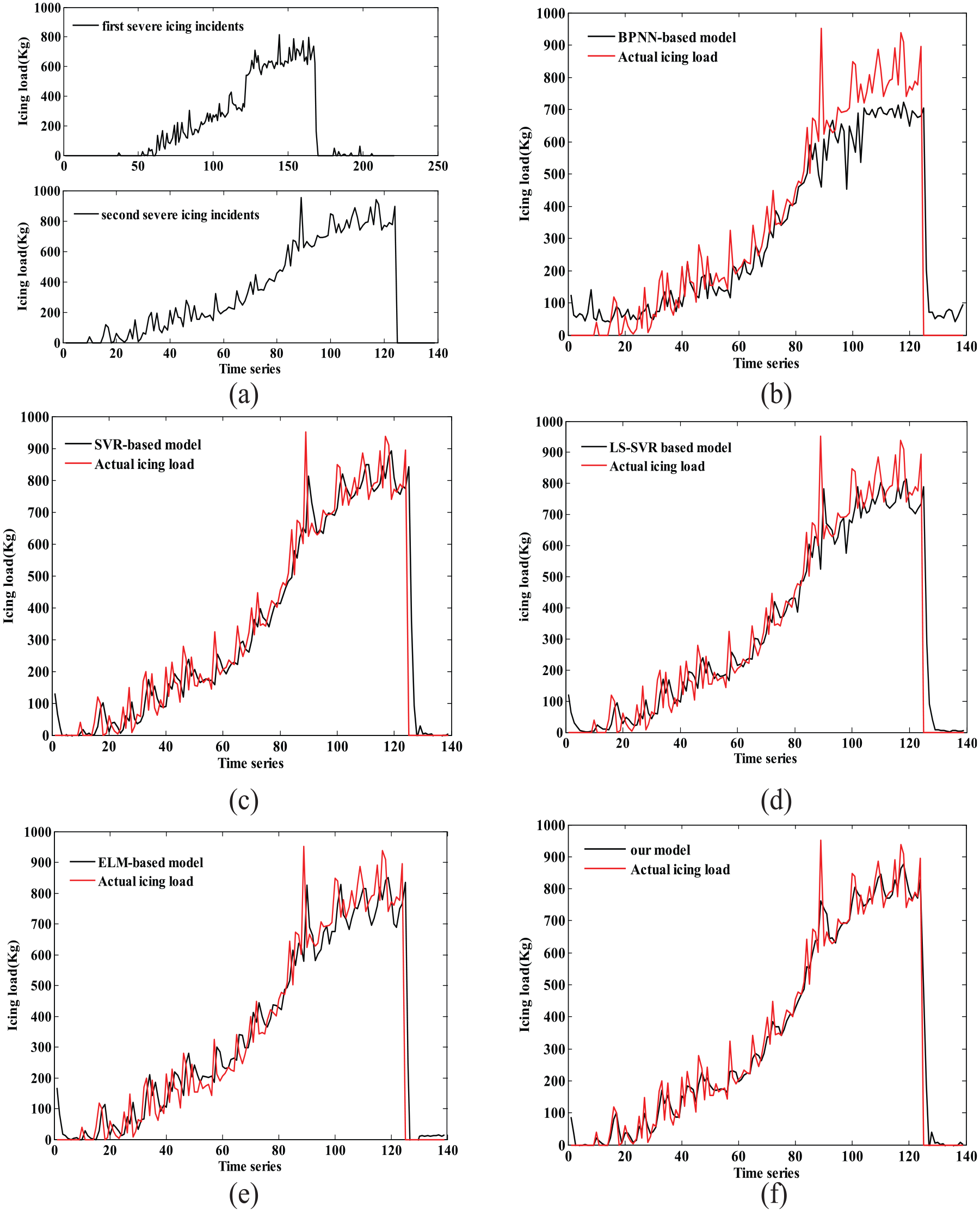
Comparison between the single-step predictions of our proposed online model and other four compared models (K = 1). (a) training and test set; (b) BPNN-based model; (c) SVR-based model; (d) LS-SVR based model; (e) ELM-based model; (f) our model.
Comparison between the mean absolute errors of predictions of our proposed online model and other four compared models (in kg).
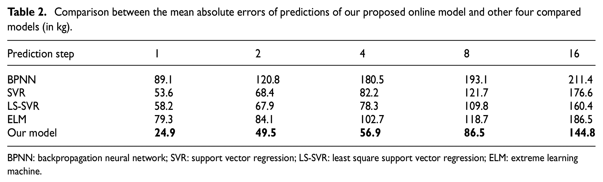
BPNN: backpropagation neural network; SVR: support vector regression; LS-SVR: least square support vector regression; ELM: extreme learning machine.
Comparison between the mean absolute errors of predictions of our proposed online model and other four compared models (in kg).
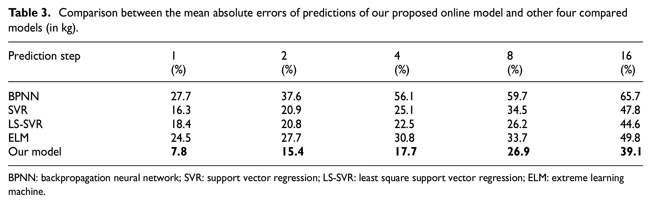
BPNN: backpropagation neural network; SVR: support vector regression; LS-SVR: least square support vector regression; ELM: extreme learning machine.
Comparison between the mean absolute errors of predictions of our proposed online model and other four compared models (in kg).
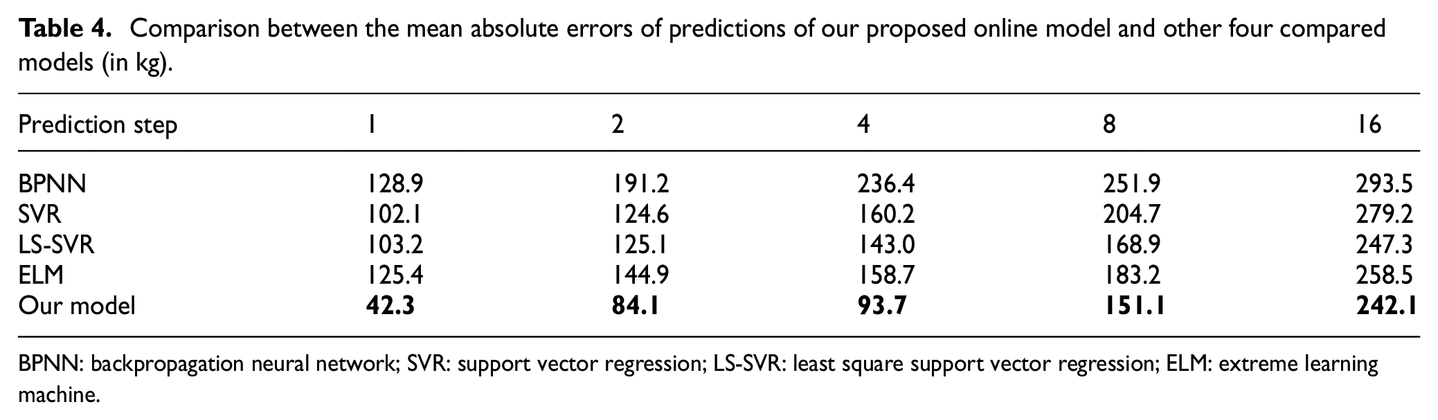
BPNN: backpropagation neural network; SVR: support vector regression; LS-SVR: least square support vector regression; ELM: extreme learning machine.
Figure 5 indicates significant differences between the single-step predictions of the BPNN-based model and the actual ice-accretion curve. Clearly, the icing-load predictions of this model cannot satisfy the accuracy requirements of the power sector for icing-load predictions. The ice-accretion curves produced by the single-step predictions of the SVR-based model, LS-SVR-based model, ELM-based model, and our model are very close to the actual ice-accretion curve, indicating that these models have high prediction accuracy. However, as the four compared icing-prediction models cannot be adjusted dynamically, its predictions are always delayed to some extent. Comparison of our proposed model with the other four compared models clearly shows that our proposed model achieves minimum MAE, MRE, and RMSE values compared to other models, which demonstrates that our proposed model can closely approximate the highly dimensional, non-linear ice-accretion process. This is attributed to the incremental algorithm, which allows our prediction model to be dynamically updated via the addition of new samples; our model is therefore able to achieve its optimal state by adjusting itself to dynamic micrometeorological inputs in real time. As a result, among the aforementioned models, our model yields the best fit with the actual data when the prediction step length is K = 1. Furthermore, the single-step predictions of our model are largely consistent with the actual state of ice accretion.
Tables 2–4 show that increases in the step length (i.e. elongation of the interval between the predictions) lead to corresponding increases in the error-related indices for all five icing-prediction models. Nonetheless, the single-step and multi-step prediction accuracies of our proposed model are uniformly superior to those of the conventional BPNN-, SVR-, LS-SVR-, ELM-based icing-prediction models. This result provides evidence for the viability and superiority of dynamic regression models.
Comparison of generalizability among five prediction models
To validate the generalizability and robustness of our prediction model, single-step and multi-step generalization was performed using historical samples from the mild icing incident (300 samples) and the second severe icing incident (139 samples) as the training and test sets, respectively. The results of the single-step generalization are shown in Figure 6, and the results of the multi-step generalization are shown in Tables 5–7.
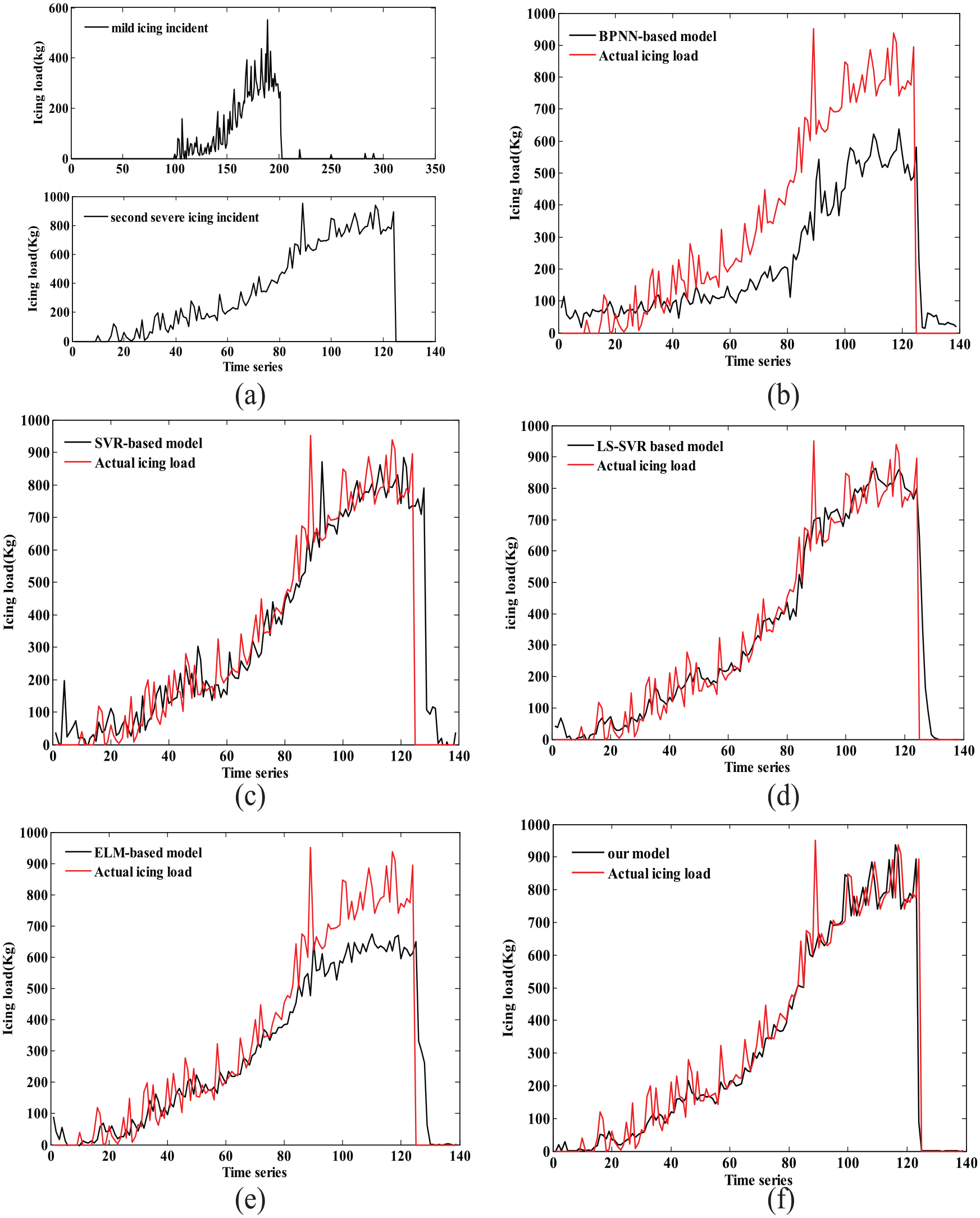
Comparison between the single-step generalizations of our proposed online model and other four compared models (K = 1). (a) training and test set; (b) BPNN-based model; (c) SVR-based model; (d) LS-SVR based model; (e) ELM-based model; (f) our model.
Comparison between the mean absolute errors of generalizations of our proposed online model and other four compared models (in kg).
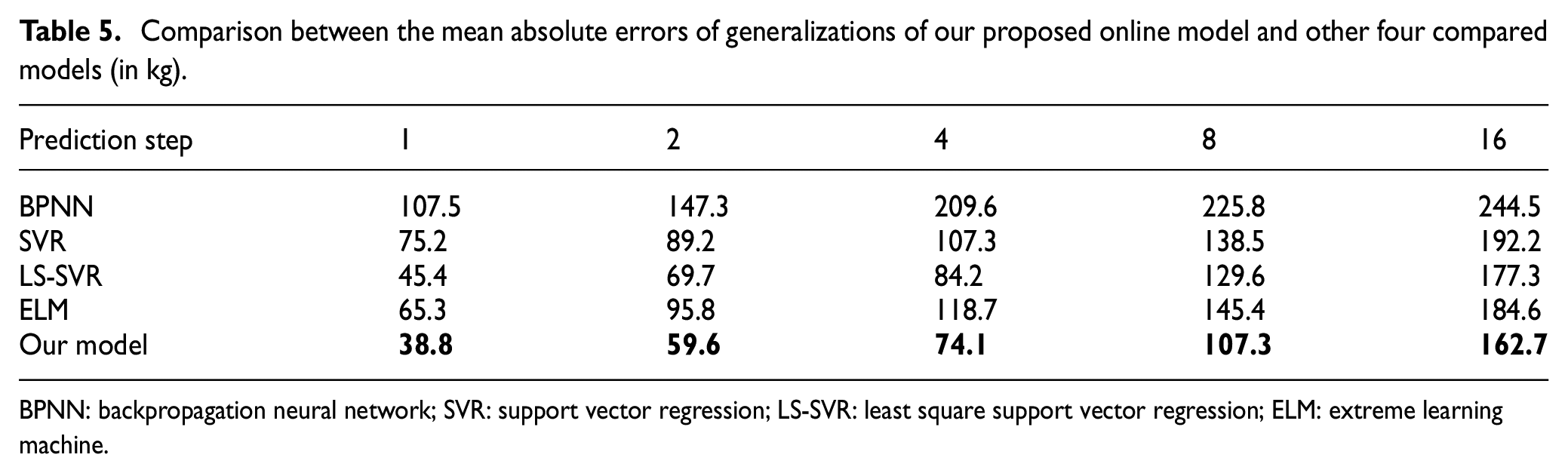
BPNN: backpropagation neural network; SVR: support vector regression; LS-SVR: least square support vector regression; ELM: extreme learning machine.
Comparison between the mean absolute errors of generalizations of our proposed online model and other four compared models (in kg).
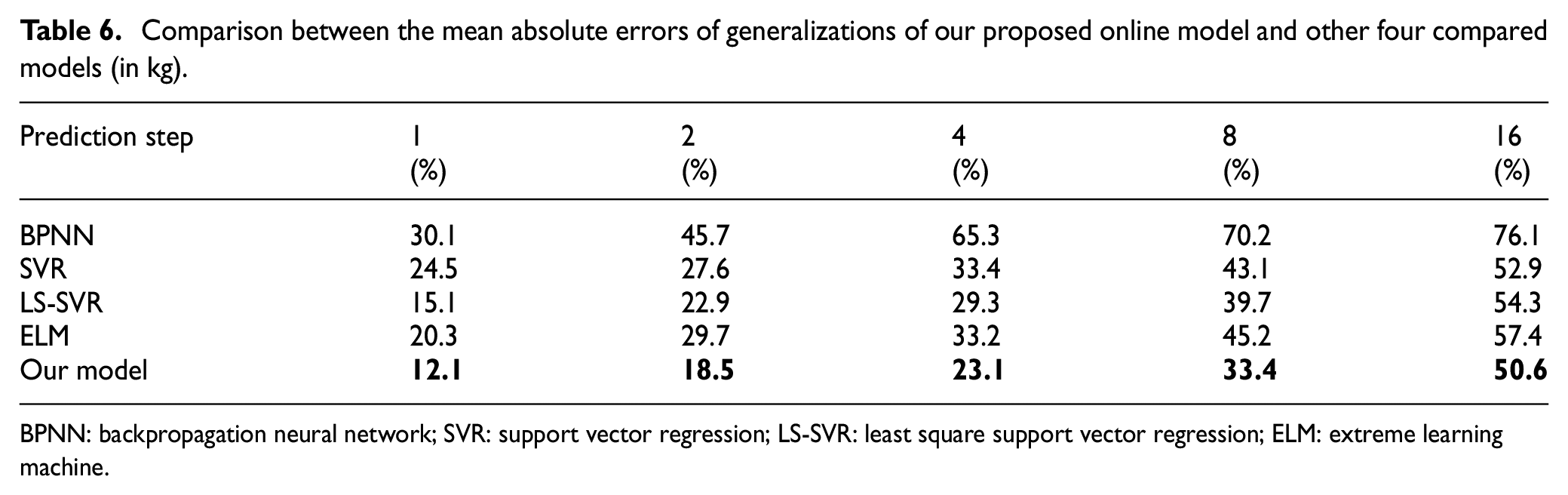
BPNN: backpropagation neural network; SVR: support vector regression; LS-SVR: least square support vector regression; ELM: extreme learning machine.
Comparison between the mean absolute errors of generalizations of our proposed online model and other four compared models (in kg).
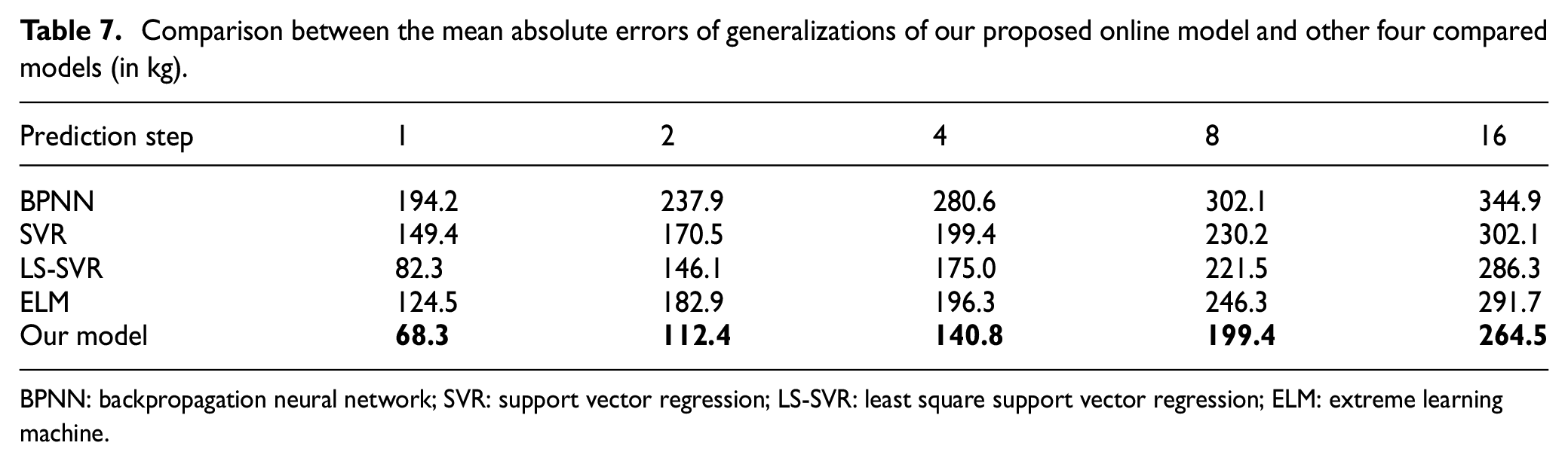
BPNN: backpropagation neural network; SVR: support vector regression; LS-SVR: least square support vector regression; ELM: extreme learning machine.
The time series representing ice accretion during the mild icing incident and the second severe icing incident are shown in Figure 6(a). The greatest icing loads for these incidents are 550.7 and 951.9 kg, respectively. Comparing the single-step and multi-step generalizations of the five models reveals that the BPNN-based regression model has the poorest generalizability. From Tables 5 to 7, it is obvious that the values of the MAE, MRE, and RMSE of the proposed model are all smaller than the other existing models in one-step-ahead to sixteen-step-ahead prediction, which further demonstrates the superiority of the proposed model’s generation ability. For instance, with respect to the BPNN, SVR, LS-SVR and ELM, the RMSE for one-step-ahead prediction was reduced by 64.83%, 54.28%, 17.01%, and 45.14%, respectively, compared to that of the proposed model. For two-step-ahead prediction, the RMSE was reduced by 52.75%, 34.08%, 23.07%, and 38.55%, respectively. For four-step-ahead prediction, the RMSE was reduced by 49.82%, 29.39%, 19.54%, and 28.27%, respectively. For eight-step-ahead prediction, the RMSE was reduced by 34%, 13.38%, 9.98%, and 19.04%, respectively. For sixteen-step-ahead prediction, the RMSE was reduced by 23.31%, 12.45%, 7.61%, and 9.32%, respectively. With the increase in the prediction horizon, the forecasting error becomes lager, but the error indices of our model are within the acceptable scale. The proposed prediction model can learn online and update its sample sets in a timely manner with the input of real-time micrometeorological data, according to the KKT conditions. In addition, the regression function and prediction model are updated by updating the sample weighting coefficients (θi). Thus, our model has a greater degree of generalizability than the conventional icing-load prediction models.
Based on the results of the proposed model and four traditional icing-load prediction models, that the proposed model outperforms the other models in both accuracies and generalizability reveals the superiority of the proposed prediction model in icing-load prediction.
Comparison of efficiency among five prediction models
To compare the efficiencies of the five aforementioned prediction models, the “tic” and “toc” commands in MATLAB for recording program execution times were used to calculate the total time cost of the prediction processes of each model. The time costs for each model in single-step, multi-step predictions and the time costs of the single-step, multi-step generalizations for each model are compared in Figure 7.
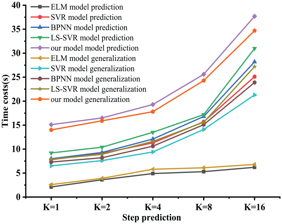
Comparison of the time cost among five different models.
Figure 7 shows that four traditional prediction models outperform the proposed online prediction model with regard to the execution efficiency, under the same operating conditions; it can also be seen that ELM-based model possesses a faster calculation speed. The high efficiencies of four compared prediction models are attributed to the batch-processing methods used in these models for their training and test sets. In contrast, our model only uses batch processing for its training set. Although the regression model does not have to be re-trained when predictions are performed on the test set, each test sample must be processed one by one, and the model must be re-optimized after each sample, increasing its time cost. Nonetheless, because the ice accretion is sampled in 20-min intervals (Δt = 20 min), the proposed regression model is perfectly viable for performing online predictions of the icing loads on transmission lines in real time.
Conclusion
We proposed a field data–driven online prediction model for the icing loads on transmission lines, which combines vast quantities of static historical data with dynamic online data using data-driven methods. The regression performance and generalizability of this model were evaluated and compared with those of current conventional prediction models. A simulation analysis based on the Tao-Luo-Xiong line of the Yunnan Power Grid in northeastern Yunnan was conducted, revealing that our model has excellent predictive capabilities and generalizability. The conclusions of this study are as follows.
Parameter optimization is important for ensuring the accuracy of the regressions for a prediction model. The use of the PSO algorithm for optimizing the regression parameters is an effective approach for avoiding optimizations to the local minima.
By combining offline modeling and online updating methods, we constructed an icing-load prediction model that can effectively estimate the ice accretion on transmission lines. The accuracy and suitability of our model were validated via comparisons with actual icing-load data. Thus, the proposed model provides a new solution for the prediction of icing loads in real time.
The predictive capabilities and generalizability of our model are superior to those of conventional icing-load prediction models. In areas where ice accretion occurs frequently, our prediction model should provide a higher level of service for guiding decisions regarding the deicing and maintenance of power transmission and transformation systems.
During the prediction-making processes of our model, all test samples participate in the incremental calculations and iterative optimizations, necessitating large-scale matrix inversions. Hence, our future research will focus on improving the execution efficiency of this model.
Footnotes
Author contributions
Y.C. and P.L. conceptualized the study, developed the software, drafted and wrote the manuscript, and reviewed and edited the manuscript; Y.C. developed the methodology; Y.C., W.R. and P.L. validated the data; W.R. and P.L. conducted the formal analysis; Y.C., W.R., and P.L. investigated the data; P.L. helped with resources, supervised the study, administered the project, and helped in the acquisition of funds; M.C. and X.S. curated the data; M.C. and X.S. visualized the study.
Authors’ Note
The data used to support the findings of this study are available from the corresponding author upon request.
Declaration of conflicting interests
The author(s) declared no potential conflicts of interest with respect to the research, authorship, and/or publication of this article.
Funding
The author(s) disclosed receipt of the following financial support for the research, authorship, and/or publication of this article: This research was funded in part by the National Natural Science Foundation of China (NSFC; 61763049) and the Science and Technology Plan of Applied Basic Research Programs Key Foundation of Yunnan province (2018FA032).