
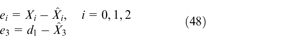
Abstract
In this paper, a strategy based on model predictive control consisting of path planning and path tracking is designed for obstacle avoidance steering control problem of the unmanned ground vehicle. The path planning controller can reconfigure a new obstacle avoidance reference path, where the constraint of the front-wheel-steering angle is transformed to formulate lateral acceleration constraint. The path tracking controller is designed to realize the accurate and fast following of the reconfigured path, and the control variable of tracking controller is steering angle. In this work, obstacles are divided into two categories: static and dynamic. When the decision-making system of the unmanned ground vehicle determines the existence of static obstacles, the obstacle avoidance path will be generated online by an optimal path reconfiguration based on direct collocation method. In the case of dynamic obstacles, receding horizon control is used for real-time path optimization. To decrease online computation burden and realize fast path tracking, the tracking controller is developed using the continuous-time model predictive control algorithm, where the extended state observer is combined to estimate the lumped disturbances for strengthening the robustness of the controller. Finally, simulations show the effectiveness of the proposed approach in comparison with nonlinear model predictive control, and the CarSim simulation is presented to further prove the feasibility of the proposed method.
Keywords
Introduction
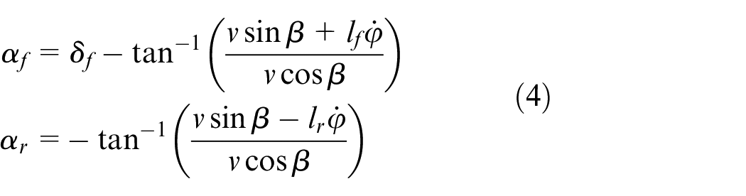
The topic of unmanned ground vehicle (UGV) 1 has become increasingly popular in the field of intelligent transportation system. In UGV application, it is inevitable that the vehicle running fast in unknown environments always encounters obstacles, 2 and the general strategy is automatic braking or active steering. In emergency situations, human drivers are accustomed to braking. However, steering or steering combined with braking would be more frequent way for the optimal maneuver. 3
Generally, obstacle avoidance steering problem is formulated as steering tracking control. 4 Naranjo et al. 5 suggest that there are two ways to design the steering controllers: imitating human drivers and using the dynamic model of the car. The former does not need detailed knowledge of vehicle dynamics, for example, proportional–integral–derivative (PID),6,7 fuzzy control,8–10 and neural network.11,12 The latter relies on the accurate dynamic model of the vehicle to build controller, such as sliding mode control,13–15 H-infinity,16,17 feedback linearization,18,19 and model predictive control (MPC).20–23 In the steering control systems, control inputs commonly consist of the steering angle and the steering torque. 24
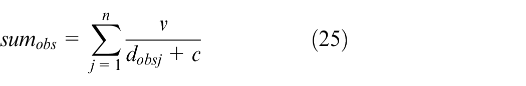
In practice, it is difficult to obtain such a safe pre-defined reference path in the unknown environment with obstacles. 25 Moreover, if the size of the vehicle is not explicitly considered, or the environment is complex and cluttered, the situation will become more serious. Thereby, path planning attracts a considerable attention in obstacle avoidance. The path planning methods are mainly classified into two categories, 26 that is, global planning method and local planning method. For the former, the UGV requires prior knowledge about the environment and assumes that the terrain is static. In contrast, the environment is partially known or completely unknown for the latter. Therefore, local path planning is more challenging. Shimoda et al. 27 propose a potential field-based path planning method for UGV to avoid static obstacles. Zhuge et al. 28 propose a dynamic obstacle avoidance algorithm using collision time histogram for UGV in uncertain dynamic environment, where the nonholonomic nature of the vehicle is embedded. Kuwata et al. 29 improve a rapidly exploring random tree approach with closed-loop prediction for obstacle avoidance navigation of the UGV in urban environment. Hao and Agrawal 30 propose a strategy based on A* search algorithm to produce the online safe path for multiple UGVs. An online autonomous navigation system of the UGV is proposed by Vilca et al. 31 for more safety and smoothness. However, most of these approaches only consider the kinematic constraints of the vehicle, and the dynamics and size of the vehicle have not been fully investigated during path computation, which weakens the feasibility of the path.
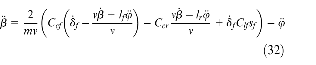
In complex traffic environment, the robustness of the control system is closely related to the safe driving of the vehicle, so that disturbance and uncertainty cannot be ignored. 32 Guo et al. 33 propose an adaptive fuzzy dynamic surface control strategy for UGV with parametric uncertainties and external disturbances. A multi-input multi-output disturbance observer is investigated for UGV steering control with multiple uncertainties. 34
Motivated by the safety and rapidity of obstacle avoidance of the UGV, a steering control strategy based on MPC, consisting of path planning and path tracking, is proposed in this paper. The path planning controller calculates the new path online according to the type of obstacles. When the obstacles are static, an optimal path reconfiguration combined with direct collocation (DC) is presented to keep the path feasible and smooth. According to Almayyahi et al., 35 most existing works have been dedicated to the navigation in static environment. For the dynamic obstacle scenario, the receding horizon control (RHC)36,37 is used for periodical path planning to ensure safety and decrease conservatism. In the road constraints, obstacle avoidance constraints and dynamic constraints are synthesized to form multiple constraint optimization problem, by which local optimal path is obtained periodically. In order to decrease the computation burden, the actual control input (front-wheel-steering angle) constraint is considered in path planning, so that the tracking design becomes an unconstrained optimization problem. To satisfy the real-time computation requirement, path tracking controller utilizes and enhances the continuous-time model predictive control (CTMPC) algorithm in Panchal et al. 38 and Lu. 39 Feedback linearization and appropriate functional expansion are used to predict the future output, and optimal control law is calculated analytically. For the lumped disturbances, the extended state observer (ESO) is introduced as estimator to guarantee the stability of the system. Finally, the simulations by MATLAB and CarSim are implemented to validate the effectiveness of the proposed method.
Comparing with the previous works, the contributions of this paper are as follows:
A judgment rule is presented to determine if there is a possibility of collision between UGV and obstacles.
The controller works more effectively on obstacle avoidance because the smooth and reasonable path has been calculated in advance.
For the computation complexity that the conventional optimization is solved at each sampling moment, the analytical control law is designed in path tracking since the path tracking constraints are taken into account in path reconfiguration priority. This greatly decreases the computation time of the tracking controller.
For the under-actuated system, CTMPC is introduced and enhanced to unify the control law with two dimensions in this paper, and the ESO is combined to reject the lumped disturbances.
This paper is organized as follows: section “UGV model” presents the bicycle dynamic model and the point mass model of UGV. In section “Obstacle avoidance steering control strategy design,” the obstacle avoidance steering control strategy is introduced. Section “Simulation” gives the simulations with static and dynamic obstacles. The conclusions are drawn in section “Conclusion.”
UGV model
Six-order dynamic model
In general, the four-wheeled dynamic model of the UGV is so complicated that precise modeling is very difficult. Hence, it is simplified into a bicycle model, 25 as shown in Figure 1. In this paper, the UGV is a front-wheel-steering vehicle, and the steering angle of the rear wheel remains unchanged.
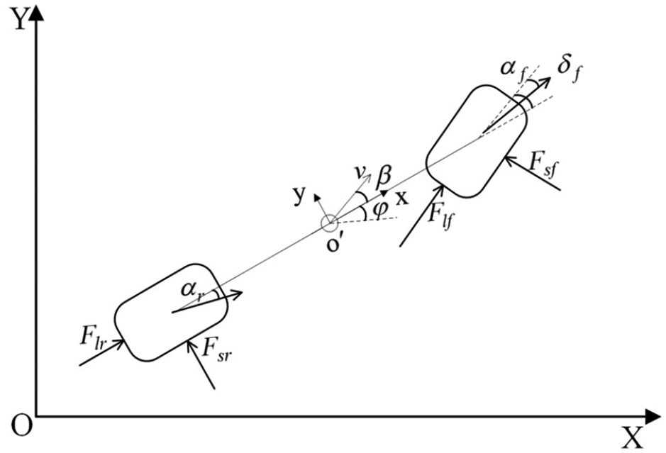
The bicycle dynamic model of UGV.
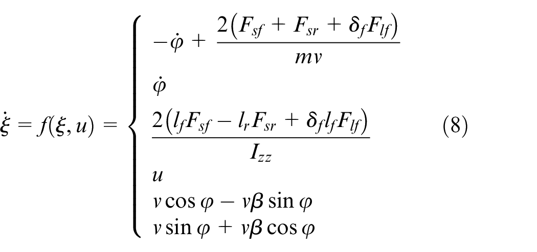
In Figure 1,
where m represents the mass of the UGV;
where
where
Assumption 1
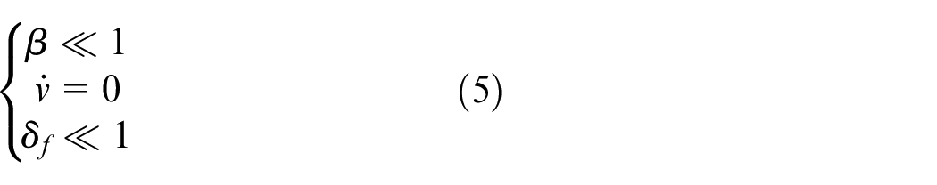
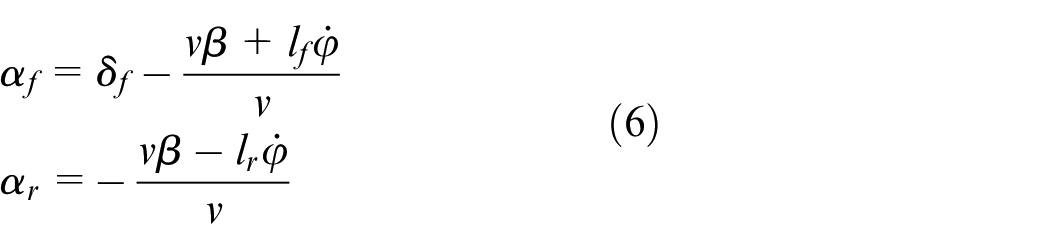
Correspondingly,
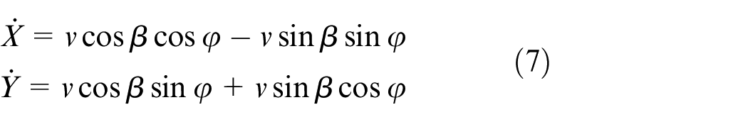
The velocity is converted into the inertial coordinate system as
Similarly, equation (7) can also be simplified in terms of Assumption 1. The state variables and control input are defined as
In order to prove that the presented approximation model is the good fidelity of true UGV dynamics, the approximation degree by the CarSim simulation is tested as shown in Figure 2.
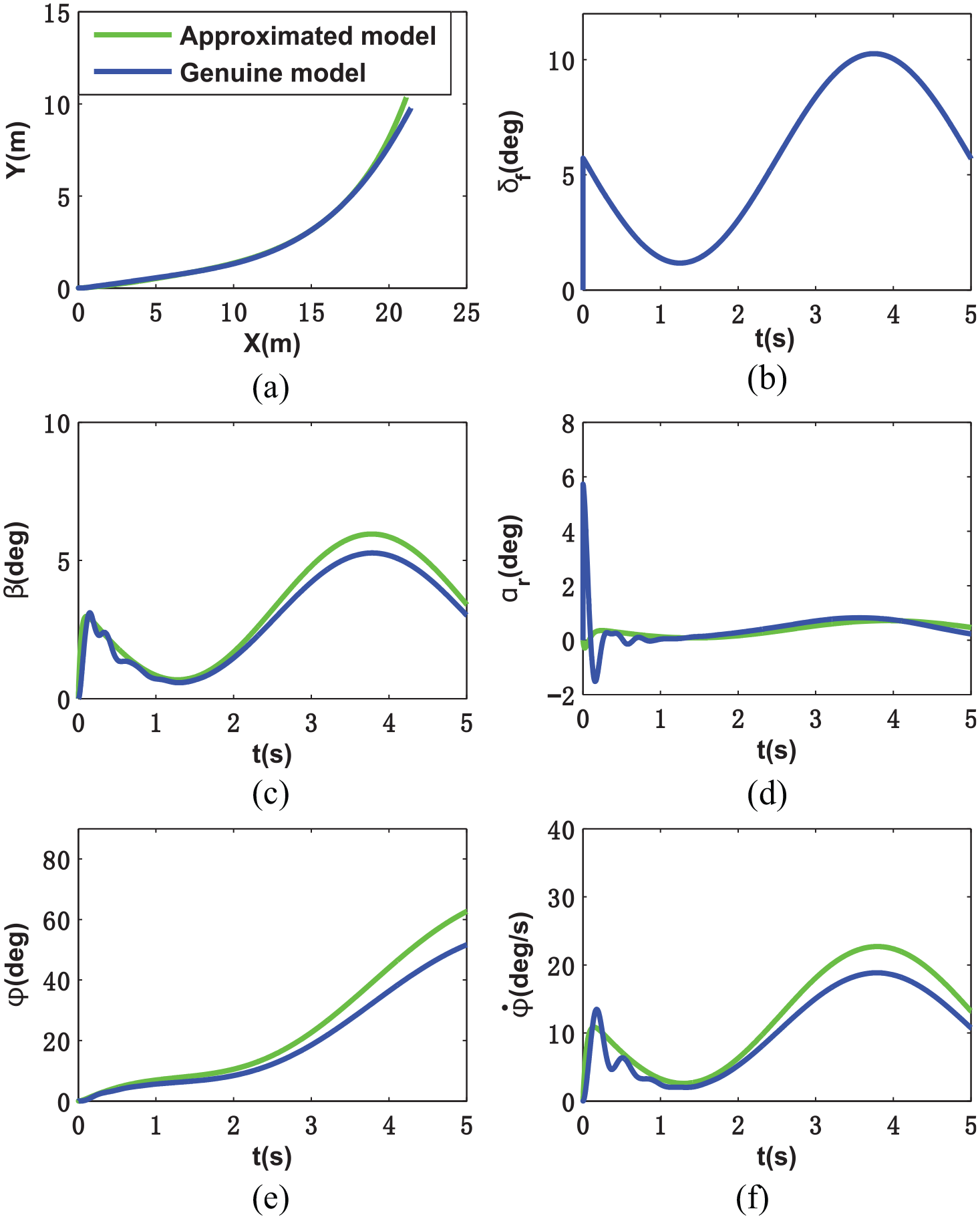
(a) The path of UGV. (b) The front-wheel-steering angle. (c) The comparison of the sideslip angles of UGV over the centroid. (d) The comparison of the sideslip angles of the rear wheel. (e) The comparison of the yaw angles of UGV over the centroid. (f) The comparison of yaw angular velocities.
From Figure 2, it can be seen that the front-wheel-steering angles of the two models change synchronously in the same sinusoidal trend. Although the other kinematic characteristics of the approximation model deviate slightly from true model, the errors are acceptable.
The point mass model
Although incorporating the dynamic model can improve the accuracy, the computation complexity increases greatly. So, the point mass model (9) of the UGV is used to calculate the path. This model is equipped with the bicycle model, also satisfying Assumption 1
where
Obstacle avoidance steering control strategy design
In order to avoid obstacles safely and quickly, the complete control system is designed as shown in Figure 3.
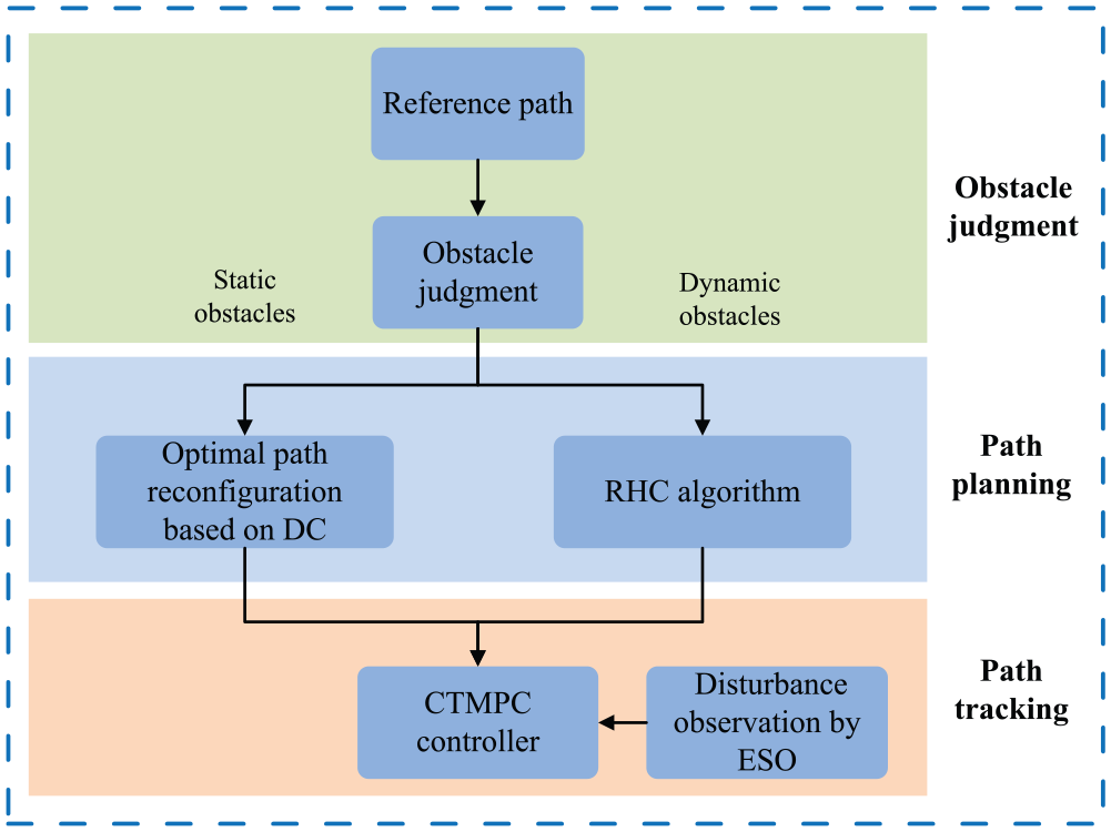
The architecture of the control system.
Generally, obstacles are divided into static case and dynamic case. When encountering obstacles, the UGV has to determine the type of obstacles at first. Then, the path planning controller is used to calculate the local path online, and the steering controller is designed to track the path precisely.
Judgment of collision possibility
In fact, the information of obstacles is unknown and uncertain. The perception technology using sensors in UGV such as lidar and camera is essential for the identification of obstacles. In addition, the multi-sensor information fusion algorithm, for example, information filter, is very useful to obtain the accurate states of the obstacle. Recently, deep learning has become the most attractive method for obstacle or target recognition. However, this paper focuses on the obstacle avoidance steering control strategy, so the states of obstacles are assumed to be known for the UGV. The following assumption is given.
Assumption 2
The position and velocity of obstacles on the road are known for UGV.
Before implementing obstacle avoidance steering control strategy, it is important to judge the collision possibility to prevent the UGV from unnecessary maneuver. The judgment rules are given as follows
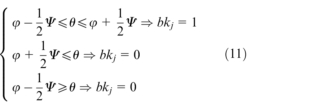
where
Judgment of the threat of obstacle.
Path planning
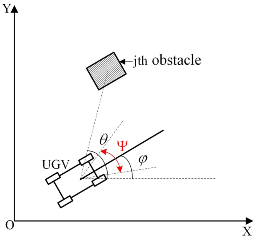
In reality, static obstacles involve broken-down vehicles, rolling stones on the highway, potholes, and so on. Dynamic obstacles mean the moving obstacles such as passersby, motorcycles, and other slow-moving vehicles. In this paper, if the decision-making system of the UGV determines that obstacles are static, the path planning controller will utilize the optimal path reconfiguration based on DC to obtain a local optimal path online. But if obstacles are dynamic, the RHC algorithm will be used in path planning for more safety and flexibility. The local path will be calculated periodically for the movement of obstacles.
Static obstacle scenario
In this scenario, the potholes on the road are taken as static obstacles, as shown in Figure 5. The optimal path reconfiguration using DC is designed to compute the local path online.
Static obstacle scenario.
The path is separated into N subintervals with equal time intervals T from
where
At each collocation point, the UGV must satisfy kinematic constraint
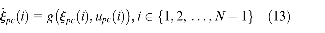
where
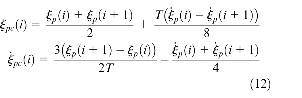
For the accuracy of the interpolation, the Defect vector needs to be 0, as follows
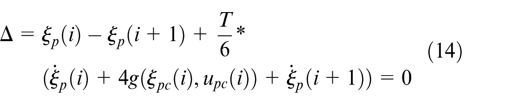
where
Combining DC, diverse constraints should be considered:
1. The input variable
where
2. The actual control input constraint
Assumption 3
There is only rolling at the junction of the tire and the road surface, and the lateral slippage does not exist. Each tire meets the rolling constraint and non-slipping constraint.
The pure rolling constraint of the rear wheel is

The non-slipping constraints of the front and rear wheels are
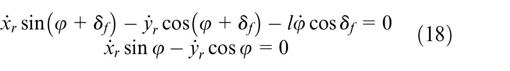
where
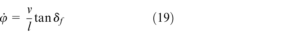
Combining with the point mass model and Assumption 1, the following equation holds
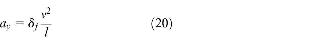
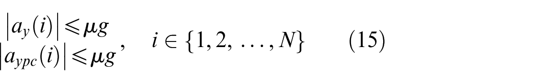
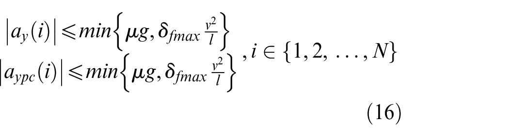
Therefore, the constraint of the front-wheel-steering angle
3. The UGV is not allowed to move across the solid lines of the lanes according to the traffic laws. Consequently, its lateral position Y should be constrained within a certain range
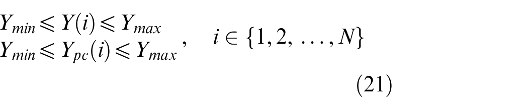
4. The UGV should always maintain a safe distance
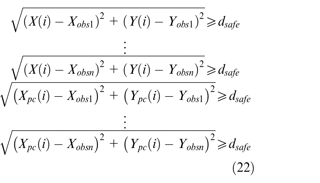
where
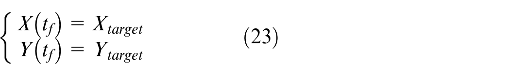
5. The UGV should arrive at the target position at time
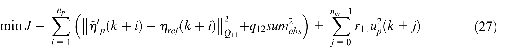
In order to smooth the path and complete the original task, the objective function of the optimal path reconfiguration method is formulated as
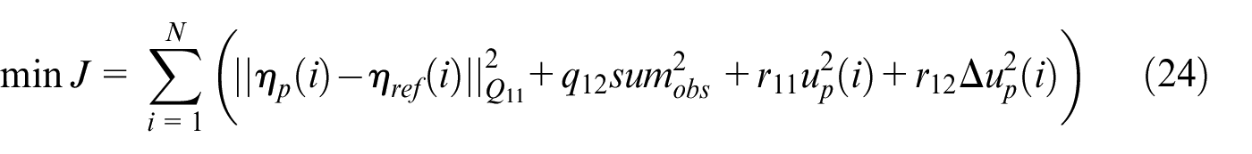
where
where
By solving equation (24) under the constraints (14)–(16) and (21)–(23), the optimal path reconfiguration can obtain N path points, that is,
Dynamic obstacle scenario
In the dynamic obstacle scenario, the UGV is cruising at the center of the lane at a constant velocity. Simultaneously, some vehicles (such as motorcycles) are moving in the same direction with slower speeds in front of the UGV, as shown in Figure 6. To overtake the running obstacles safely, RHC is used to calculate the local optimal path during each planning period.
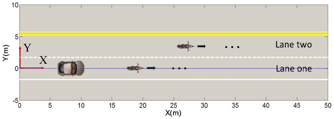
Dynamic obstacle scenario.
First, the point mass model is discretized at time k, and the state variables in
Here, RHC is used to optimize the obstacle avoidance path, as follows. In Figure 7, the solid lines represent the parts of the path being tracked, and the dash lines are the parts not tracked.
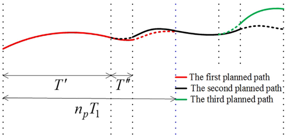
The schematic of RHC path planner.
For the dynamic obstacles, RHC focuses on avoiding obstacles and maintaining the original task, but the item about
where
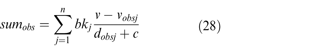
where

where
Furthermore, in order to reduce the calculation time, the reference path is directly taken as the output of the path planning controller if obstacles are far away from vehicles, that is,
By solving equation (27), the local optimal path can be obtained as the point set, that is,
Path tracking
CTMPC
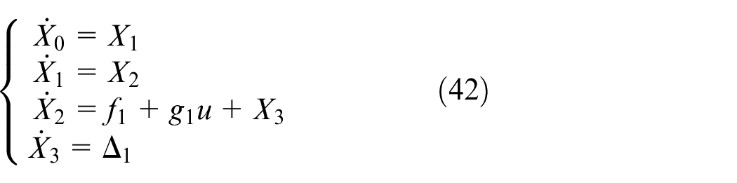
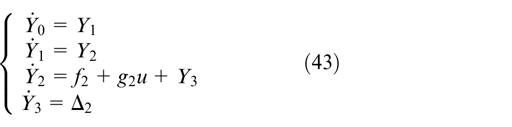
First, the following feedback linearization is implemented for dynamic model
where
The control input appears in
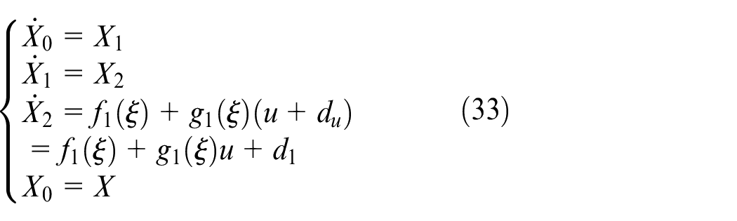
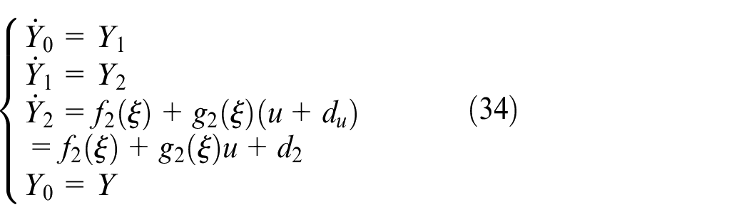
where
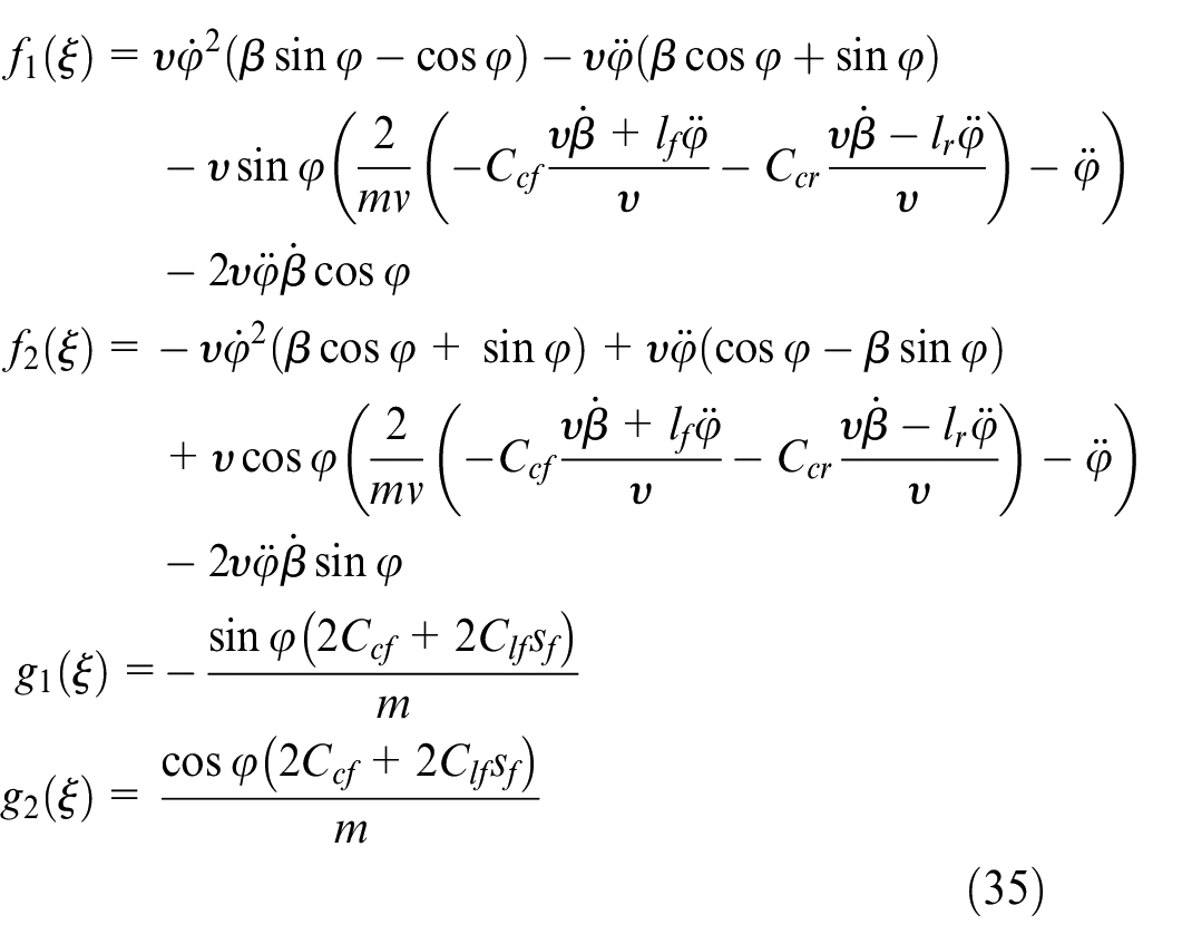
It is obvious that the UGV is an under-actuated system. Therefore, CTMPC38,39 is introduced and enhanced in this paper.
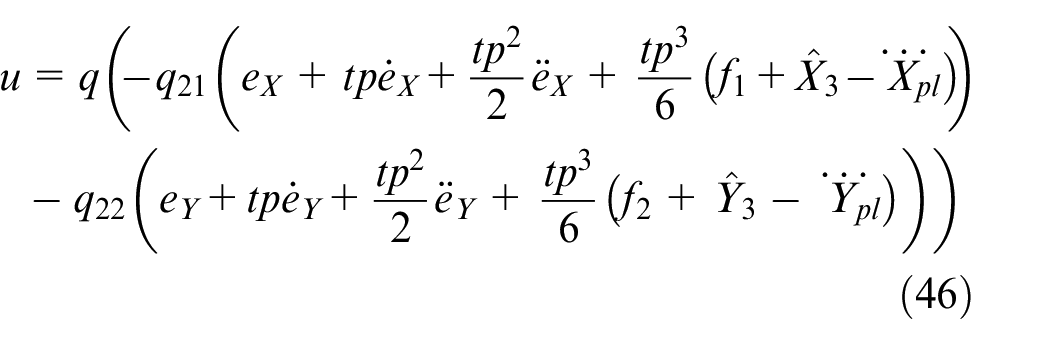
The motion of the UGV is predicted using the Taylor expansion principle based on the linearized model
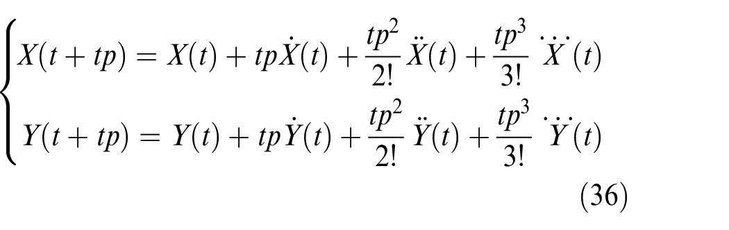
where tp is the Taylor expansion time. In order to ensure good approximation performance, tp should be small enough.
In path planning, the control input constraint has been considered so that CTMPC becomes the unconstrained optimization problem. This makes the iterative computation of control input be the analytical calculation, which reduces the computation greatly. Different from the conventional CTMPC, the tracking performance of X and Y is synthesized to form the cost function
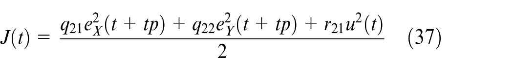
where
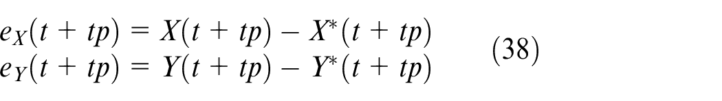
where
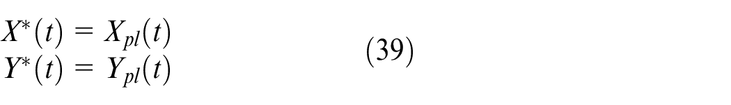
The unique control input is obtained by solving
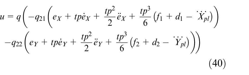
where
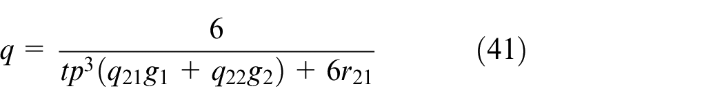
Because
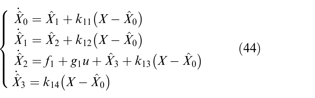
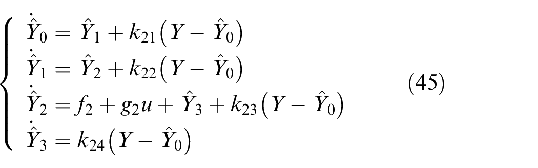
Disturbance observation by ESO
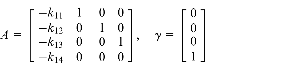
UGV hardware system is quite complex, and the environment is varying, which results in various disturbances on the control system. This may cause the UGV to sideslip or overturn. In this paper, the effect of the rough and uneven roads on the vehicle suspension system, the influence of wind resistance on the steering system, and the existence of gear meshing clearance are considered as the source of external disturbances. Therefore, ESO is designed to observe them. By taking the lumped disturbance as an extended state variable, the extended system is presented as
where
where
With
Assumption 4
Theorem 1
If the lumped disturbances satisfy Assumption 4, the observation error of the ESO is bounded.
Proof
We can get the following differential equations about the observation errors at X from equations (42) and (44)
where
The differential equations are transformed into the following
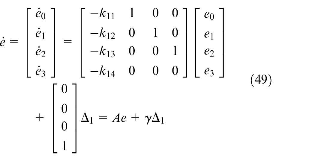
where
Solving equation (49), yields
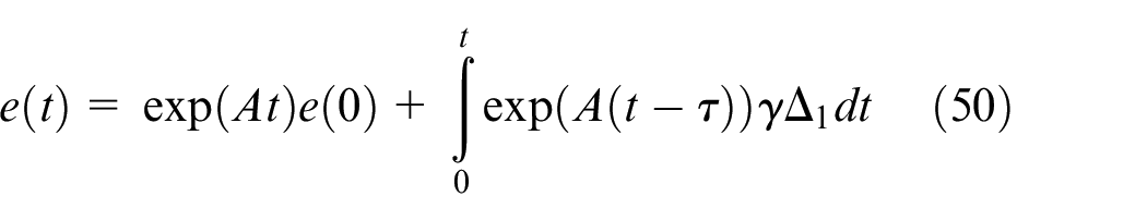
We can obtain the eigenvalues of the matrix A, and mark them as
According to Assumption 4, there is
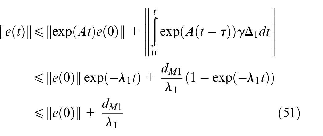
which means that the observation errors of the ESO are bounded. By choosing the suitable observer gains, the observation errors can converge to the origin point
Assumption 5
Theorem 2
If the lumped disturbances and the path variables satisfy Assumptions 4 and 5, and the controller parameters are selected properly, the path tracking error is bounded, and the whole control system is stable.
Proof
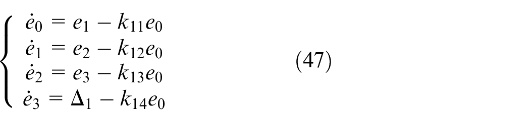
Substitute equation (46) into equations (33) and (34), and subtract the nominal system, then the error state equation is formulated as
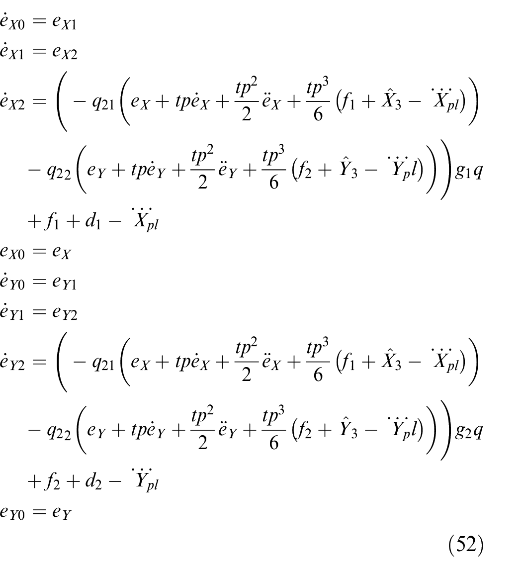

where
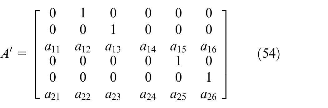
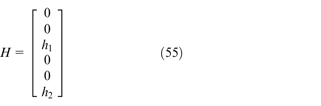
Select the appropriate parameters
Algorithm
The algorithm of the proposed obstacle avoidance steering control strategy is listed as follows:
Step 1. Judge the collision possibility of the obstacles. If there is a possibility of collision, go to next step, otherwise skip to Step 3.
Step 2. Use suitable planning methods for the different types of obstacles to optimize the local obstacle avoidance path online and then go to Step 4.
Step 3. Instead of planning a new local path, take the reference path directly as the output of the path planning controller.
Step 4. Use the CTMPC algorithm based on ESO to track the local path. At the next time, return to Step 1.
Simulation
The scenarios of the static obstacles and dynamic obstacles are used to demonstrate the steerability of the proposed obstacle avoidance control strategy. In this paper, the numerical simulations using MATLAB and CarSim are proposed to prove the effectiveness and feasibility of the proposed method. Table 1 shows the dynamic parameters of the UGV.
Dynamic parameters of the UGV.
UGV: unmanned ground vehicle.
Static obstacles
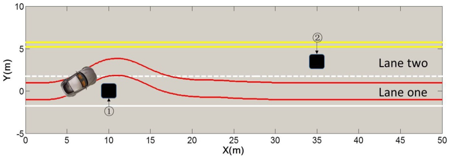
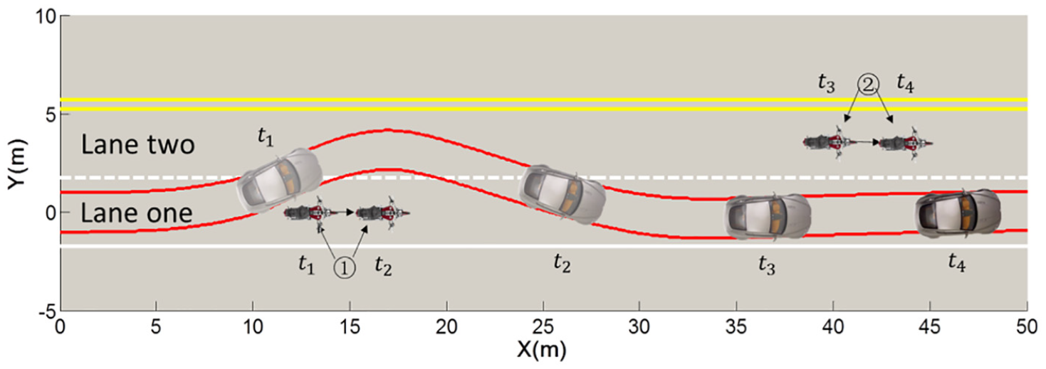
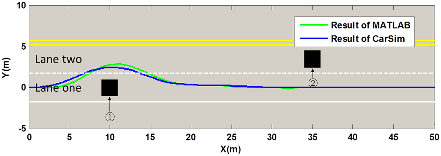
In static obstacle scenario, there are two lanes marked as lane one and lane two, respectively, in the same direction. The length of the road is 50 m, and the width of each lane is 3.5 m. The origin of the inertial coordinate system is located at the starting point of the centerline of the lane one. There are two potholes at (10, 0) and (35, 3.5) marked as ① and ②, respectively, and their length and width are both 1.6 m. The width of the UGV is 2 m. Before encountering the obstacles, the UGV is cruising at lane one at 5 m/s. Simultaneously, the sinusoidal term
The parameters related to the constraints are as follows:
First, the UGV computes a local path using the optimal path reconfiguration based on DC as shown in Figure 8, in which N = 40. The red path represents the computed result using the point mass model. It can be seen that this path maintains the adequate safe distances from the obstacles and satisfies the road constraint. Moreover, the UGV keeps cruising on the lane one after avoiding the first obstacle. As shown in Figure 9, the input in the optimization problem also meets the dynamic constraints. It is obvious that there is no risk of sideslip or rollover, that is, the UGV is stable.
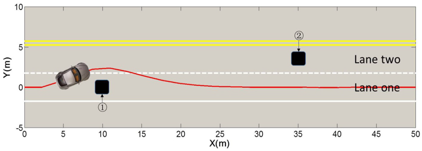
Path planning in static obstacle scenario.
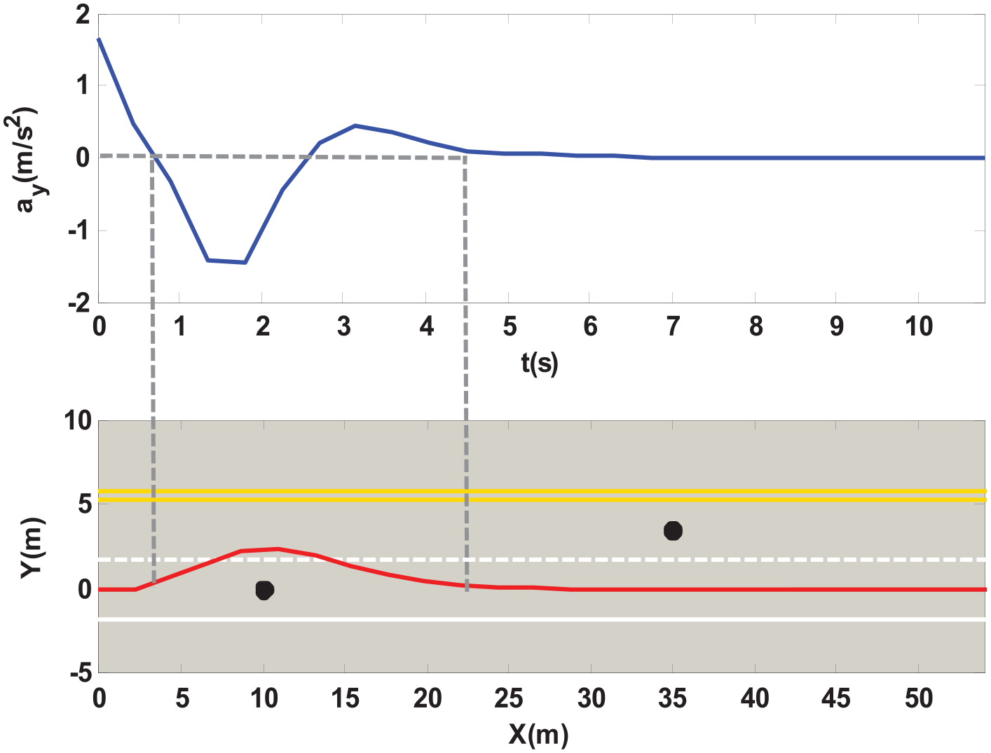
Lateral acceleration.
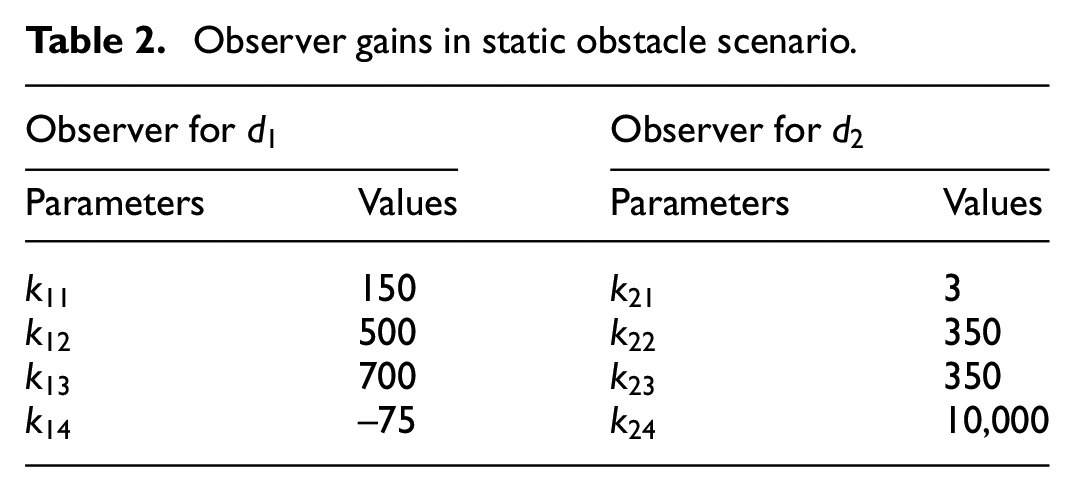
Second, in the path tracking controller design, the Taylor expansion time is 0.45 s. The observer gains are chosen as shown in Table 2, and the lumped disturbances are observed as shown in Figure 10.
Observer gains in static obstacle scenario.
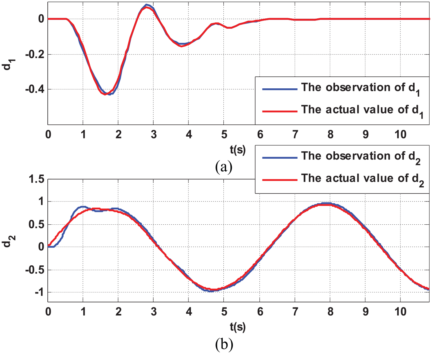
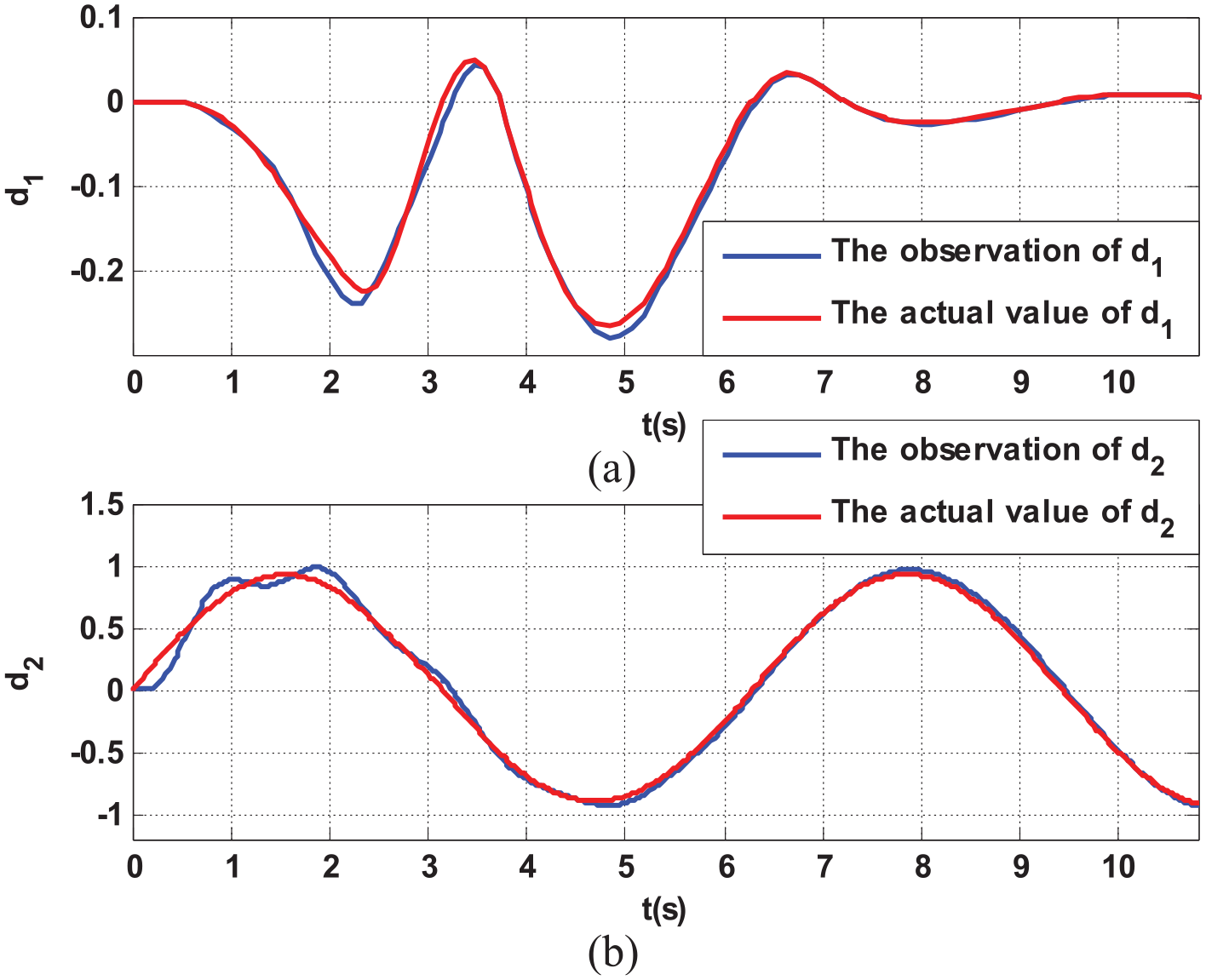
(a) The observation of d1 in static obstacle scenario. (b) The observation of d2 in static obstacle scenario.
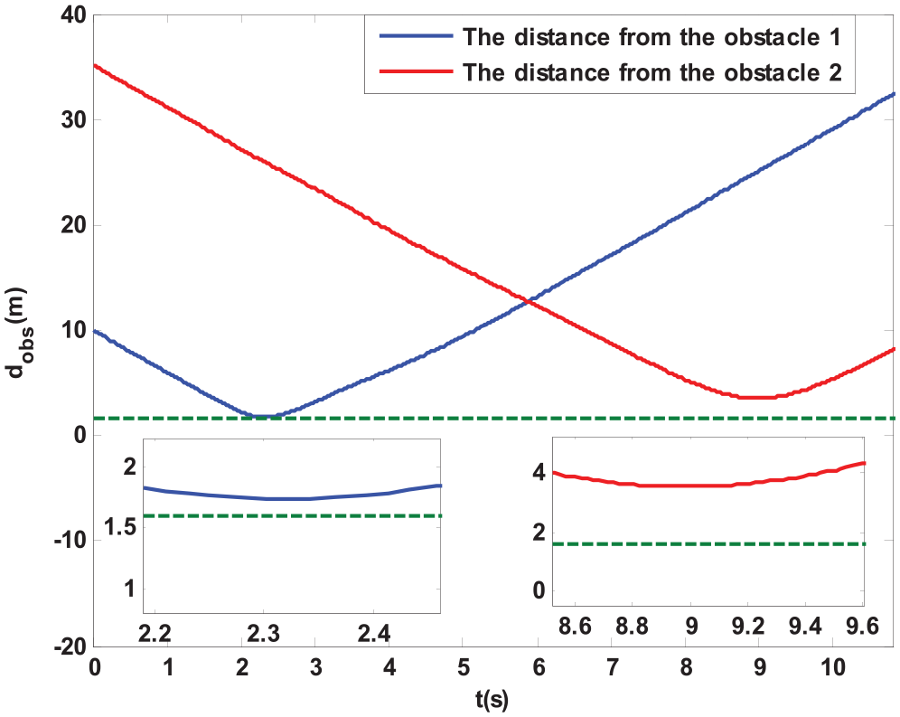
We can see that both observers can converge to the actual disturbances. Figure 11 shows the tracking performance. The red lines represent the left and right outer boundaries of the UGV. The UGV adopts detour strategy after judging that the obstacle ① poses a risk to the current driving. However, the extra detour is not implemented after determining that the obstacle ② is not threatening. Furthermore, the designed control system can effectively suppress the disturbance and maintain the UGV stability. As shown in Figure 12, UGV always keeps the safe distance, that is, 2 m to two obstacles.
Outer boundaries of UGV path tracking in static obstacle scenario.
The distance from obstacles in static obstacle scenario.
In order to illustrate the effectiveness of the proposed control method, a comparison simulation with dynamic-model-based nonlinear model predictive control (NMPC) 42 method is carried out as shown in Figures 13 and 14.
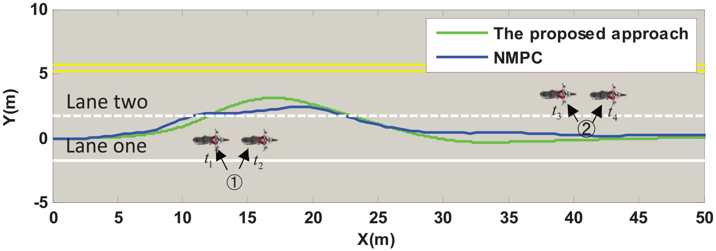
Obstacle avoidance comparison at the centroid of UGV with NMPC in static obstacle scenario.
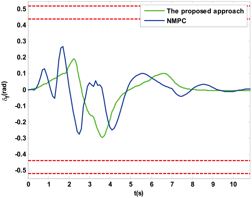
Control input comparison with NMPC in static obstacle scenario.
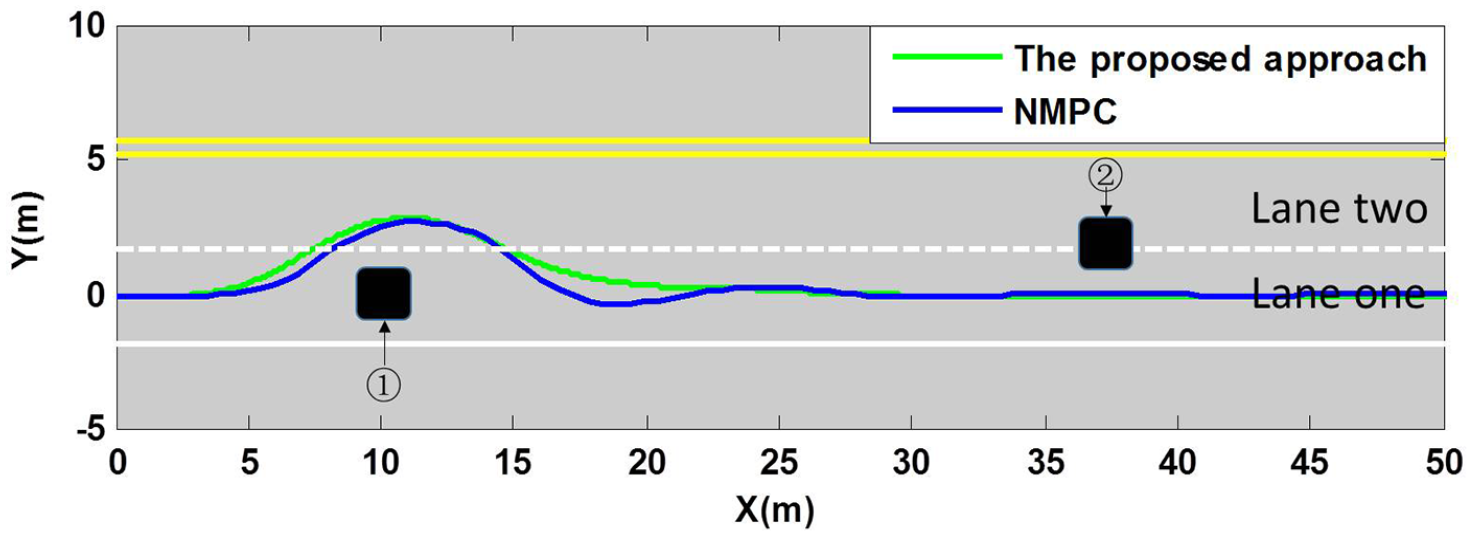
The centroid coordinates in the course of vehicle driving are shown in Figure 13. Although the two methods can successfully avoid the obstacles, the vehicle does not swing in the proposed method after getting around the obstacles. Moreover, the proposed method spends 19.09 s in calculation, but the traditional NMPC takes 241.92 s under the same conditions. The constraint of
Dynamic obstacles
In dynamic obstacles scenario, the length of the road is still 50 m, and the width of each lane is 3.5 m; there are two motorcycles driving at 1 m/s in the same direction with the UGV in both lanes, whose initial positions are at (10, 0) and (35, 3.5); their length and width are 1.6 m and 0.7 m, marked as ① and ②, respectively;
In the path computation, the sampling period is 0.45 s; the predictive period is six steps, and the control period is four steps. The planning cycle is 1.8 s.
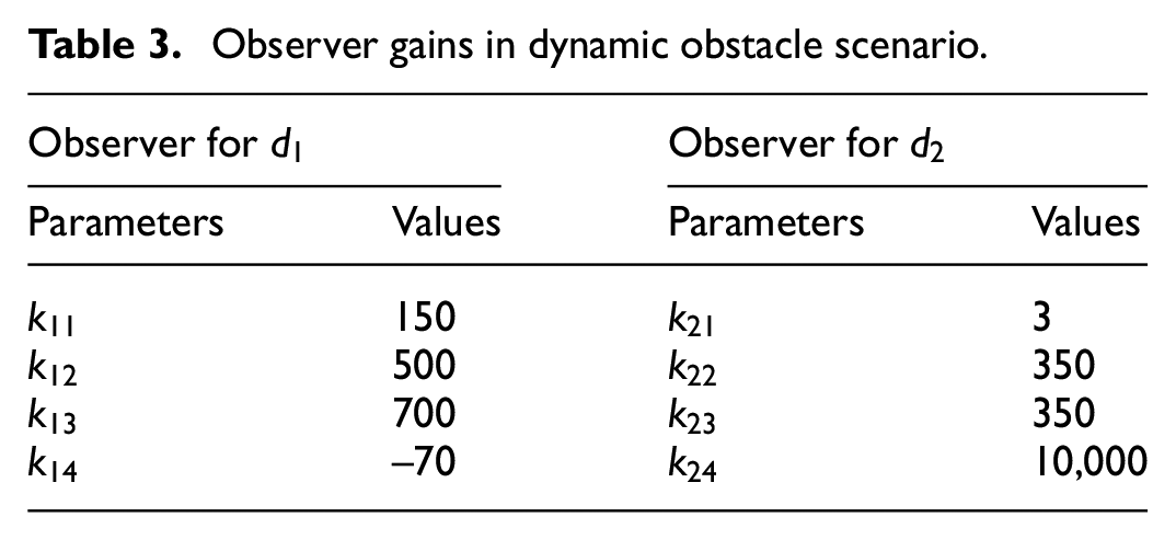
In the path tracking, the Taylor expansion time is 0.9 s. The CTMPC controller and ESO are designed. The observer gains are chosen as shown in Table 3. The disturbances are observed as shown in Figure 15.
Observer gains in dynamic obstacle scenario.
(a) The observation of d1 in dynamic obstacle scenario. (b) The observation of d2 in dynamic obstacle scenario.
It can be seen that after a certain time period, both observations can still converge to the actual disturbances like that in static obstacle scenario. Figure 16 shows the tracking result.
Outer boundaries of UGV path tracking in dynamic obstacle scenario.
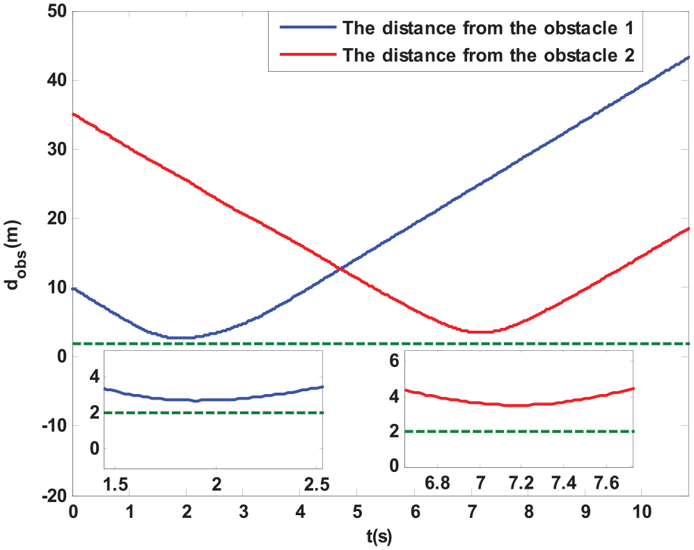
At time
The distance from obstacles in dynamic obstacle scenario.
The comparison between the proposed method and traditional NMPC in dynamic obstacle scenario is shown in Figures 18 and 19. In the traditional NMPC, the swing behavior of the UGV still exists. In this simulation, the proposed method spends 31.24 s, and NMPC uses 303.42 s.
Obstacle avoidance comparison at the centroid of UGV with NMPC in dynamic obstacle scenario.
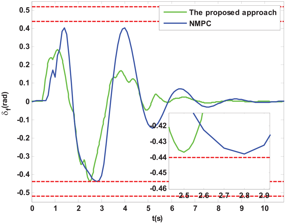
Control input comparison with NMPC in dynamic obstacle scenario.
The control inputs are shown in Figure 22. The trend of the control input in the proposed method is much smoother than that of NMPC. That is the variance of the control input of NMPC is still larger. We can get the same conclusion as the static obstacle scenario from Figures 18 and 19.
CarSim simulation
In order to verify the performance of the proposed method in realistic environment, CarSim and MATLAB are combined to give the joint simulation results. The dynamic characteristics are established in CarSim. The position information of the obstacles is the same as the static and dynamic obstacle scenarios in MATLAB simulation. The vehicle model is chosen as B-class, Hatchback, which is consistent with the dynamic parameters in this paper. To clarify the difference between CarSim joint simulation and MATLAB simulation, the result of the former is called CarSim, and the latter is called MATLAB.
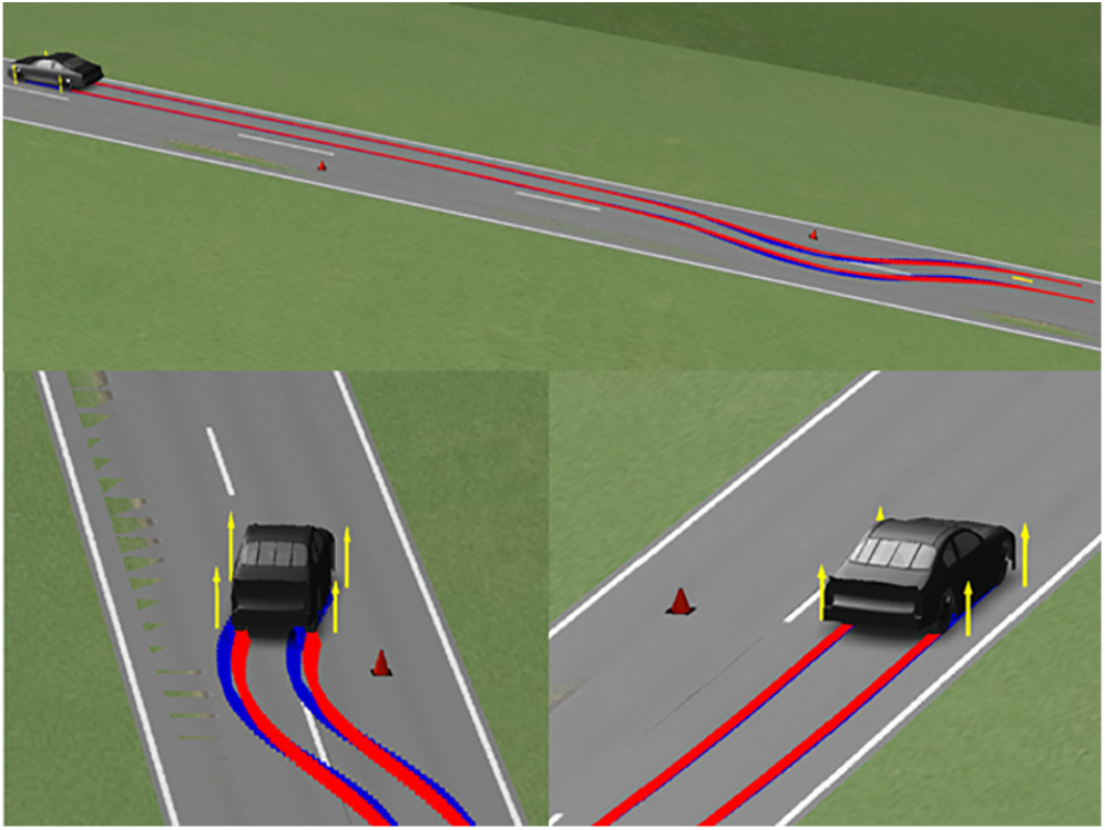
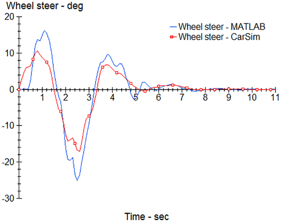
In static scenario, cones are used to take place of the potholes in Figure 20 for the reason that there are no potholes in the animator of CarSim. Figure 20 demonstrates the actual trajectory of the vehicle, and it is obvious that the vehicle succeeds in avoiding the static obstacles. Figure 21 shows the simulation comparison between using CarSim and MATLAB, which shows the effectiveness of the proposed method both in simulation and experiment scenarios. Figure 22 gives the control inputs using CarSim and MATLAB, respectively, where the control inputs have the similar behavior.
Path tracking of UGV by CarSim in static obstacle scenario.
Obstacle avoidance comparison at the centroid of UGV using CarSim and MATLAB in static obstacle scenario.
Control input comparison using CarSim and MATLAB in static obstacle scenario.
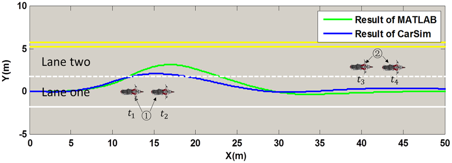
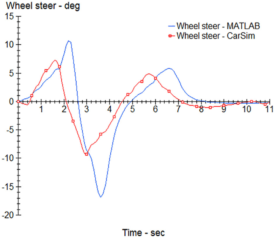
Figures 23–25 demonstrate the control performance of the proposed method using CarSim simulation in dynamic obstacle scenario. Figure 23 shows the real trajectory of the vehicle. It can be seen that the vehicle can avoid the moving obstacles in the road without collision. Figure 24 presents the simulation comparison between using CarSim and MATLAB. The UGV can successfully avoid the dynamic obstacles and keep 1.6 m distance from them, which satisfy the constraints. The control inputs are depicted in Figure 25, and they have similar curves. This verifies the effectiveness of the proposed method in more realistic scenario.
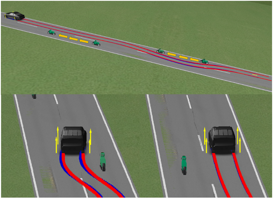
Path tracking of UGV by CarSim in dynamic obstacle scenario.
Obstacle avoidance comparison at the centroid of UGV using CarSim and MATLAB in dynamic obstacle scenario.
Control input comparison using CarSim and MATLAB in dynamic obstacle scenario.
Conclusion
For more safety and flexibility, a strategy for the complex obstacle avoidance steering control problem of the UGV is designed in this paper. According to the type of obstacles, an optimal path reconfiguration based on DC and RHC are proposed, respectively. Different from the previous path planning algorithms, our algorithms take into account the constraint of the actual control input. The unconstrained CTMPC controller is designed to make the tracking system have better real-time performance. The ESO is introduced to observe the disturbances to guarantee the stability and robustness of the control system.
Footnotes
Declaration of conflicting interests
The author(s) declared no potential conflicts of interest with respect to the research, authorship, and/or publication of this article.
Funding
The author(s) disclosed receipt of the following financial support for the research, authorship, and/or publication of this article: This work was supported by the National Natural Science Foundation of China (Nos 61773279 and 61873340), the Open Project of Key Laboratory of Micro Opto-Electro Mechanical System Technology, Tianjin University, Ministry of Education (No. MOMST 2016-4), and Joint Science Foundation of Ministry of Education of China (No. 6141A0202304).