Sage Journals: Discover world-class research

Abstract

This paper studies the behaviour of circular tunnel subjected to dynamic excitation. Tunnels with three different diameters were selected to perform the shake table test at three different covers. The dry sandy soil was used for testing. The mechanical properties like Young’s modulus and shear modulus of sand was calculated from bender element test. The soil–tunnel interface coefficient was calculated from the direct shear test. The soil pressure generated due to dynamic loading were measured by soil pressure transducers. The actual motion of shake table was captured by hand-held vibration analyser. The tunnel was placed parallel and perpendicular to the direction of shaking. The three-dimensional finite-element model was developed for tunnel with both the orientations. The tunnel was assumed to be elastic. Dry sand was assumed to follow non-linear elasto-plastic material using Mohr–Coulomb failure criterion with non-associated flow rule. The results obtained from numerical analysis are compared with experimental results and are expressed in the form of peak dynamic stresses. The time history and fast Fourier transform results of dynamic stresses are also compared. It shows reasonable agreement with both values. Finally, the seismic design guidelines for tunnel are suggested.

Keywords

Shake table tunnel finite-element method absorbing boundary bender element

Introduction

An earthquake occurs due to sudden release of energy, resulting in seismic wave generation. These waves cause large damage to infrastructure when it reaches to the ground surface. Circular tunnels are often constructed for highways, railways, water conveyance in hydro power projects and metro projects. These tunnels are mainly excavated using tunnel boring machine or drill and blast methods. Earlier, theses tunnels were constructed in sound rock with high cover. However, due to rapid urbanization and urgent need of society, there is an increase in the demand for underground structures like tunnels. In addition, tunnels are now being constructed in high seismic zones with soft ground condition, mainly in soil. The safety of the tunnel is very important during adverse loading conditions. This demands more focused research to understand the behaviour of tunnels subjected to seismic loading.

Earlier, underground structures were considered safe during the earthquake. However, failure of underground structures during the Kobe earthquake (1995, Japan), Chi-Chi earthquake (1999 Taiwan) and Kocaeli earthquake (1999 Turkey) changed the belief among researchers. Almost seven tunnels experienced serious damage during Kobe earthquake, 93 tunnels were affected during the 1923 Kanto earthquake, and Niigataken-Chuetsu earthquake affected 24 tunnels.¹ The damage occurred either due to large deformation or due to liquefaction of surrounding soil. Poor geological conditions, shallow depth of tunnels and the presence of active faults were the main reason for the damage of underground structures. While seismic excitation of tunnel induces axial and curvature deformation in longitudinal direction, it induces ovaling or raking in transverse direction, depending on the shape of the tunnel. Axial and curvature deformations were reported in tunnels placed along the longitudinal direction of shake table shaking.² Moreover, lack of suitable guidance in most of the cases lead to inefficient design by professionals. Full dynamic analysis should be done to know the effect of soil–structure interaction. Simplified dynamic analyses should be used for preliminary design.

In the field, modern instruments like load cell and pressure cell provide useful data and insight into the behaviour of underground structures. It is comparatively convenient to use the instruments and sensors installed on site to get the load and pressure data of tunnel in case of static analysis. However, it is not as convenient to measure dynamic forces at the site because high magnitude earthquakes are rare and vibration from other sources also affects the dynamic force measurement significantly. Sensors for dynamic measurement should be carefully selected to avoid measurement issues.³ Care should be taken to select the scale of an experimental model to predict the behaviour of prototype.⁴ To overcome this limitation of field data, lab tests were performed on models.

Experimental and numerical simulation of the tunnel has been investigated by many researchers.^5–12 A series of shake table test of the utility tunnel in transverse and longitudinal direction was performed; the results show that the amplification factor of soil decreases with increase in peak ground acceleration (PGA) due to soil non-linearity,⁷ and high-intensity shaking generates some residual stress in the tunnel.¹⁰ The acceleration response of tunnel is higher than surrounding soil for high shaking.⁶ Under seismic loading, the tunnel vibrates in rocking mode, and racking¹³ also bending deformation occurs in the tunnel.⁶ However, most of the researchers are more focused on internal forces, deformation and acceleration developed in tunnel during seismic activity, very few studies have been carried on the stresses generated in the soil during earthquake. Since, the value of soil pressure exerted on tunnel is used by the designer for support design of tunnels. This study is more focused on the soil pressure generated during the earthquake.

Frictional characteristics of the interface between soil and tunnel significantly affect load transfer mechanism between soil and tunnel. To design tunnel for seismic loading, closed form solutions are available for full slip and no slip interface condition, and the designed tunnel is to be checked for both the cases. However, partially slip interface condition may generate higher forces in tunnel.¹⁴ Therefore, the closed form solution cannot predict the actual behaviour of tunnel during seismic loading, and full dynamic analysis should be performed.¹⁵

In this paper, the 1g shake table test was performed on the circular tunnel subjected to dynamic loading. The test was performed with different tunnel diameters at different covers. The dynamic pressure developed due to seismic force in dry sand is measured by soil pressure transducers. In addition, the actual motion of shake table is captured by hand-held vibration analyser. The soil–tunnel interface value was calculated by direct shear test. Furthermore, the numerical model was established in the finite-element model. The results obtained from numerical analysis was compared with experimental results and are expressed in the form of percentage change in peak dynamics stresses with respect to static pressure on the tunnel. The time history and fast Fourier transform (FFT) results of dynamic stresses are also compared.

Experimental setup

Shake table

The shake table used for testing is unidirectional with table top dimension of 1.5 m × 1.5 m (Figure 1). The motion of table is constrained to one-dimension only. The lateral displacement of shake table is given through an electric motor of 15-HP capacity. The maximum displacement of shake table is ±50 mm and maximum frequency is 10 Hz under ideal conditions. The maximum load-carrying capacity of shake table is 2000 kg. However, increasing the load or displacement of shake table decreases the frequency. Therefore, for the present test, the displacement was set to ±5, ±10, ±15, ±20, ±25 and ±50 mm, whereas the frequency was set 0.5, 0.8, 1.5 and 2.0 Hz. It should be noted that 2.0 Hz frequency is available for only ±5 mm displacement, whereas for ±50 mm displacement 0.5 and 0.8 Hz frequencies are only available.

Figure 1.

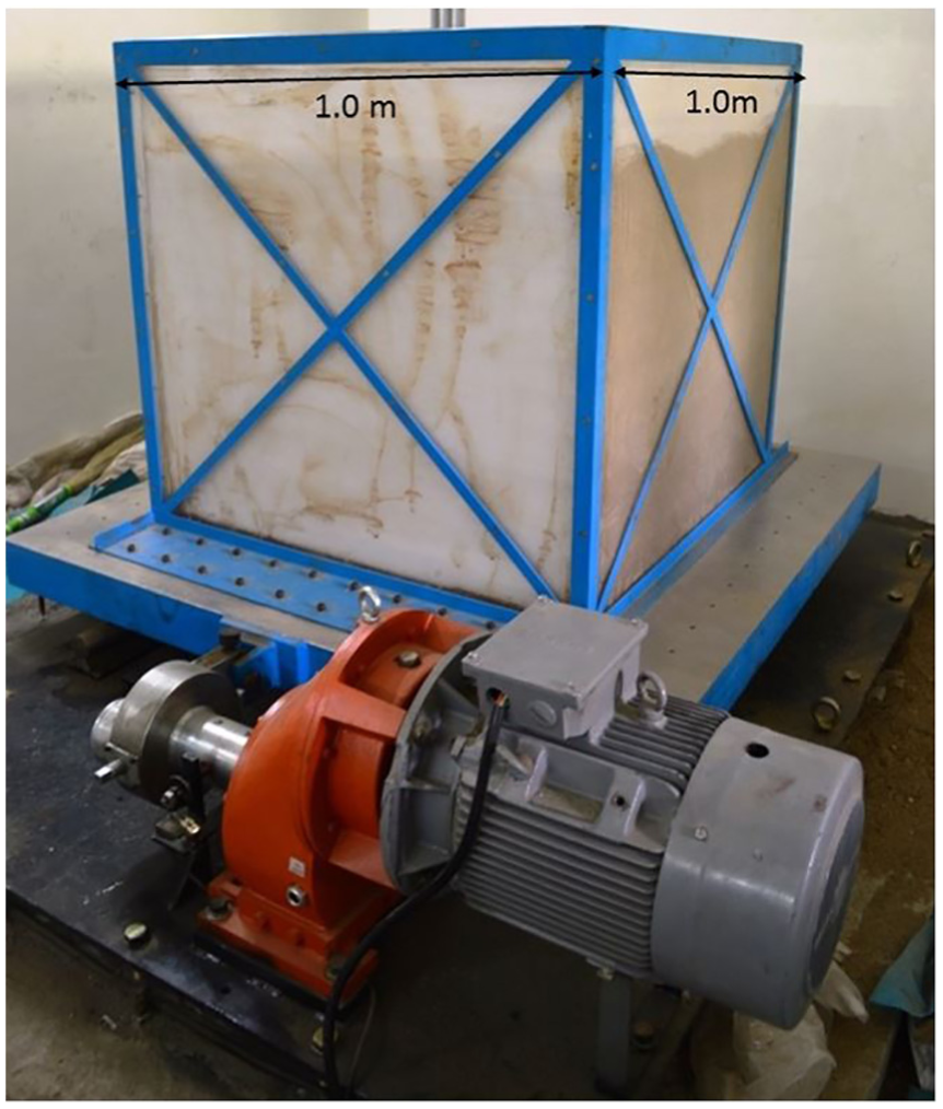
Shake table with container.

Soil container/tank

The rigid type container was used for experiment. The internal dimensions are 1.0 m × 1.0 m × 1.0 m, and it is firmly fixed to the shake table. It was fabricated using perspex glass of 18 mm thickness and strengthened using flat and angle structural steel sections (Figure 1). The expanded polyethylene (EPE) foam was used on the inner boundary of the container, perpendicular to the direction of shake table movement. The base was made rough by sticking sand using industrial adhesives.

Sensors setup

Two types of sensors were used to find the seismic response of the tunnel. The hand-held vibration sensors with magnetic tip were placed at the centre of the vertical boundary of the container/tank (Figure 2). The hand-held vibration analyser was used to capture the actual motion of the shake table.

Figure 2.

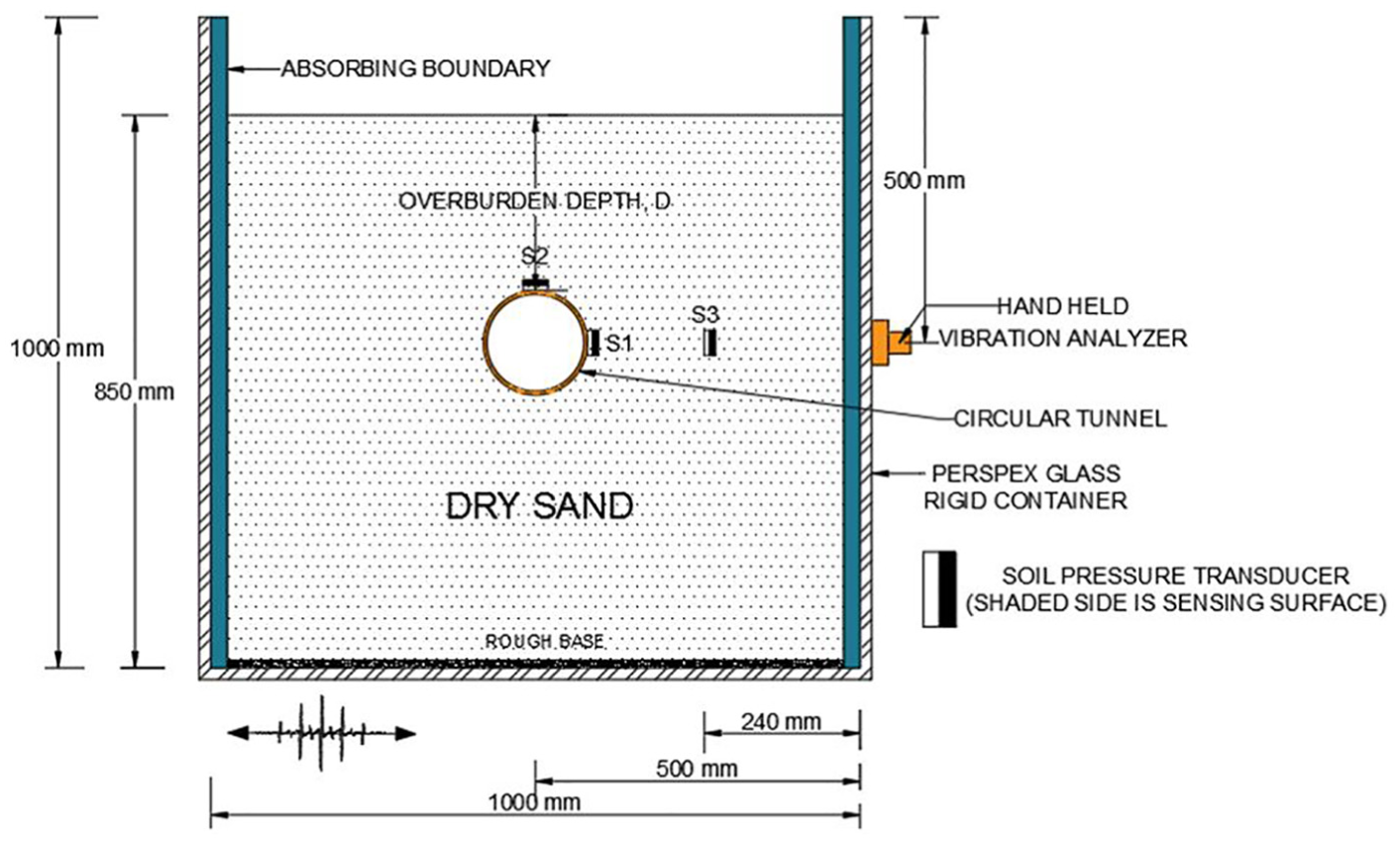
Experimental setup and arrangement of sensors for transverse direction of tunnel.

Three soil pressure transducers were used to measure the pressure in the soil and on tunnel. The data were recorded on the dynamic data acquisition module. The arrangements of sensors are shown in Figures 2 and 3.

Figure 3.

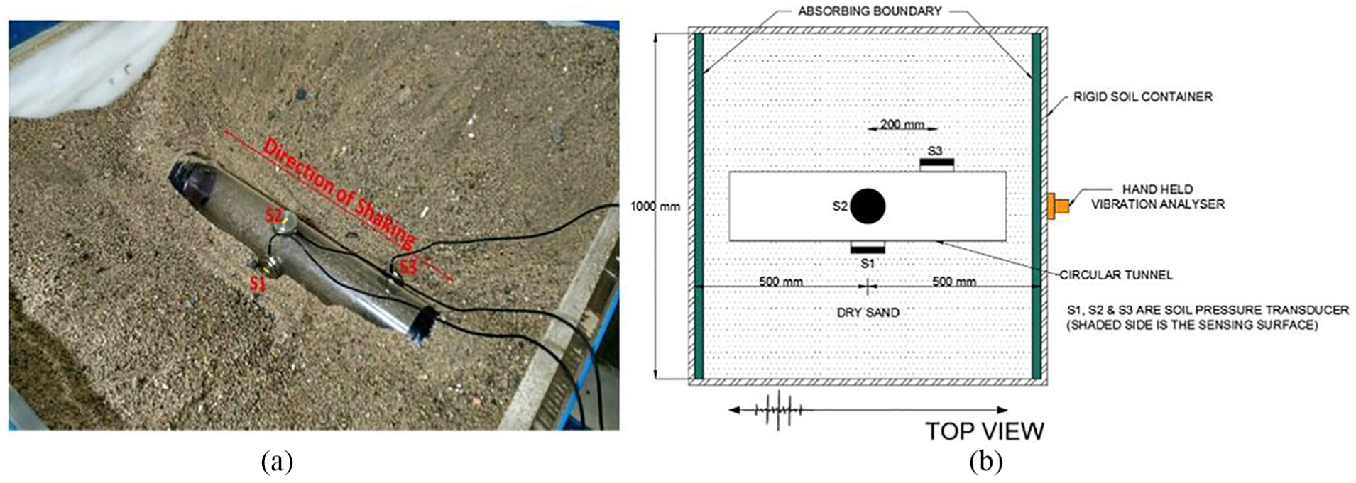
Arrangement of sensors for longitudinal orientation of tunnel: (a) experimental and (b) graphic diagram.

Methodology

Soil filling in container/tank

The dry sandy soil was used as fill material for a tunnel in the shake table experiments. Permanent changes can appear in internal forces because of densification of sand layer during intense shaking.⁵ Therefore, prior to start of the actual test, the sand is compacted to its maximum possible density, to avoid sand densification during the test. To achieve this, the sand was placed loosely by air pluviation, then the vibration was given from shake table. Three layers of sand were chosen for simplification in the analysis. Total five such trials were made. It was observed that during shaking, the sand densification occurs (12%–18%). After sand densification, the densities at the middle of each layer were measured and found to be 1.55, 1.65 and 1.75 g/cm³ (Figure 4). The overall depth of the sand layer is 85 cm. To achieve the desired density, the soil in the container was divided into three layers: top and middle layer having a thickness 28 cm and bottom layer thickness as 29 cm. The target was set to maintain the sand density at 1.55, 1.65 and 1.75 g/cm³ for top, middle and bottom layers, respectively. Additional tamping was done to achieve the desired density. After this arrangement, the sand densification during the test nearly ends. Therefore, for numerical modelling, the sand layer is divided into three parts, and the density in the middle of each layer is considered for the analysis (Figure 4).

Figure 4.

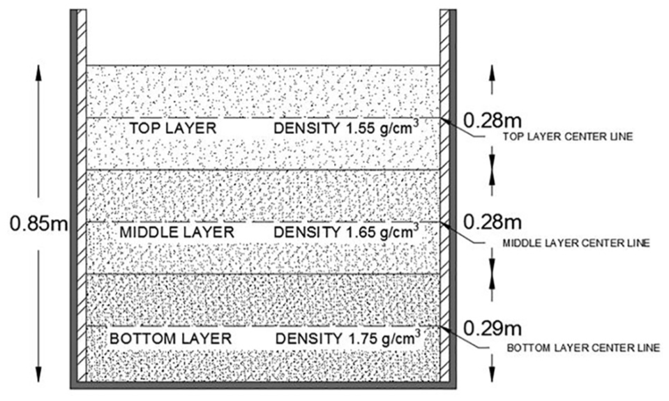
Dry sand layers.

The tunnel was made up of perspex glass having an outer diameter of 10, 15 and 20 cm with thickness of 3, 3 and 6 mm, respectively. The shake table experiments were conducted by placing the tunnels in parallel and perpendicular (Figures 2 and 3) to the direction of shaking (one at a time) at three different covers.

Absorbing boundary

The effect of artificial boundaries of a soil container on dynamic response of soil can be significant if not designed properly. Use of absorbing material on boundary is recommended for minimizing the boundary effect. The commercially available EPE foam panel was used as the absorbing boundary in the present tests. These foams were placed on both inner sides of the end walls of the soil container, perpendicular to the shaking direction. The thickness of foam was designed as per practical guidelines provided by Lombardi; for this case, it is 25mm. The design criteria used here are based on impedance. For good absorbing boundary, the impedance of soil should be greater than 200 times the impedance of foam.¹⁶

To determine the damping associated with foam, the hysteresis loss of energy in the foam was calculated as per ASTM D 3574-17 (Figure 5). The compression force displacement (CFD) procedure was followed.¹⁷ The hysteresis loss calculated as per equation (1) is 25%

\begin{matrix} Hysteresis loss = \frac{A_{1}}{A_{1} + A_{2}} \end{matrix}

(1)

where A₁ is the area in between loading–unloading curve, and A₂ is the area under unloading curve.

Figure 5.

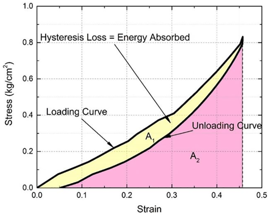
Hysteresis loss in foam.

Material properties

The bender element test was done to get the mechanical properties like Young’s modulus, shear modulus and Poisson’s ratio of sand and foam. Figure 6 shows the test results obtained from bender element. In this test, the p-wave and s-wave velocity is computed by dividing the length of sample with time taken by waves reach from the source end to receiver end. Time taken to reach from source to receiver was the difference between the arrival times of the first peak at receiver end to the peak at source end. For present test, the sample length was 12.0 cm and diameter 6.0 cm. These dimensions are selected to obtain the best results from bender element tests as a slenderness ratio greater than 2 gives best results.¹⁸ However, bender element source and receiver ends have the outward projection of 1.5 mm each. Therefore, tip-to-tip distance between source and receiver is 11.7 cm. The test was conducted for different densities of sand like 1.55, 1.65 and 1.75 g/cm³. The dilatation angle of dry sand was assumed to be 1°. In addition, the value of D₆₀, D₃₀ and D₁₀ was 0.85, 0.65 and 0.45 mm, respectively.

Figure 6.

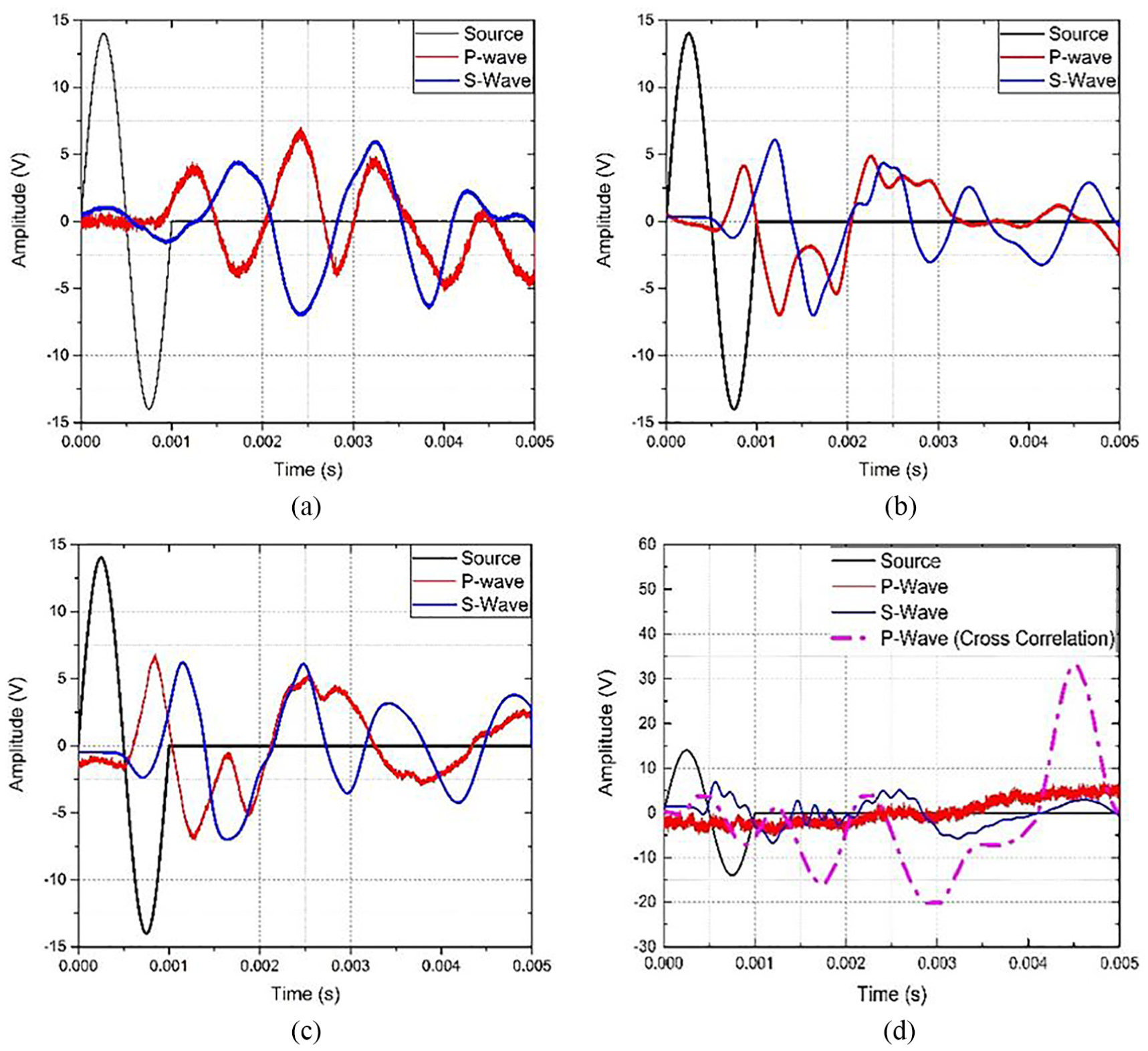
Bender element test results: (a) sand 1.55 g/cm³, (b) sand 1.65 g/cm³, (c) sand 1.75 g/cm³ and (d) foam.

The bender element can be used for materials treated with air foam, that is, the material having greater quantity of air voids.¹⁹ The test similar to the sand was performed on industrial foam which was used as absorbing boundary. Here, the tip-to-tip distance between source and receiver is 6.2 cm. For industrial foam, the s-wave is showing the peak clearly. However, the p-wave obtained during the test does not show any peak. Therefore, the method of cross-correlation was used on p-wave to find the p-wave velocity (Figure 6(d)).

Based on the p-wave and s-wave velocity obtained from bender element test, the shear modulus, Poisson’s ratio and Young’s modulus of the materials is calculated using equations (2)–(4), respectively

\begin{matrix} G = V_{s}^{2} ρ \end{matrix}

(2)

\begin{matrix} ν = \frac{{(\frac{V_{p}}{V_{s}})}^{2} - 2}{2 {(\frac{V_{p}}{V_{s}})}^{2} - 1} \end{matrix}

(3)

\begin{matrix} E = \frac{V_{p}^{2} ρ (1 + ν) (1 - 2 ν)}{1 - ν} \end{matrix}

(4)

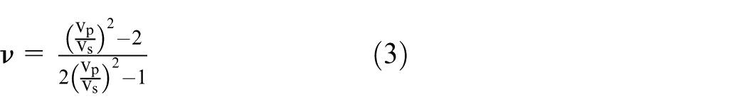
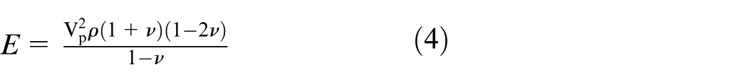
where G is the shear modulus, ρ is the density of the material, V_s is s-wave velocity, ν is Poisson’s ratio, V_p is p-wave velocity and E is Young’s modulus.

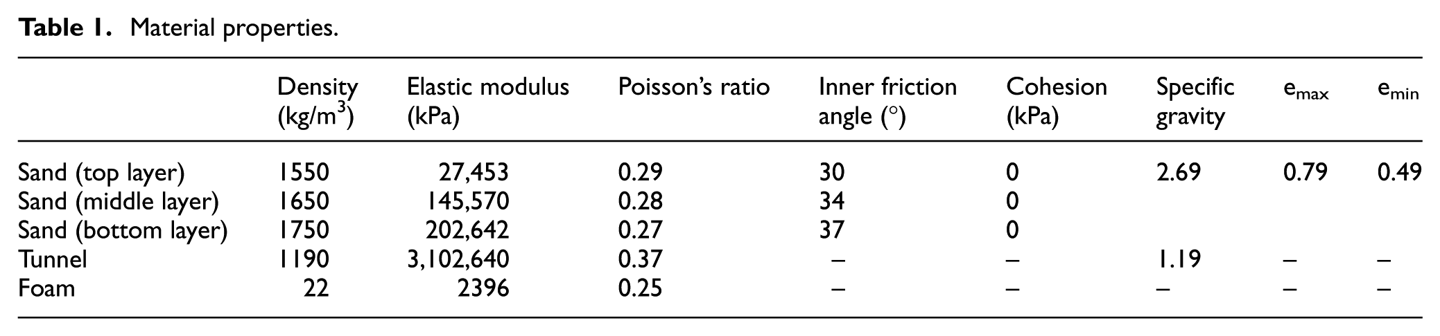
Tensile test was conducted on perspex glass rod to calculate Young’s modulus of the tunnel and container. Table 1 shows the properties of various materials used in the experiment.

Table 1.

Material properties.

	Density (kg/m³)	Elastic modulus (kPa)	Poisson’s ratio	Inner friction angle (°)	Cohesion (kPa)	Specific gravity	e_max	e_min
Sand (top layer)	1550	27,453	0.29	30	0	2.69	0.79	0.49
Sand (middle layer)	1650	145,570	0.28	34	0
Sand (bottom layer)	1750	202,642	0.27	37	0
Tunnel	1190	3,102,640	0.37	–	–	1.19	–	–
Foam	22	2396	0.25	–	–	–	–	–

The value of soil–tunnel interaction coefficient is calculated by performing the direct shear test. The dimension of the direct shear box is 6 cm × 6 cm with a height of 2.4 cm. The perspex glass plate of thickness 12 mm was placed on the lower side of the direct shear box, and the upper part is filled with the sand with 90% of relative density (Figure 7). The soil–tunnel interface coefficient of friction was calculated to be 0.12.

Figure 7.

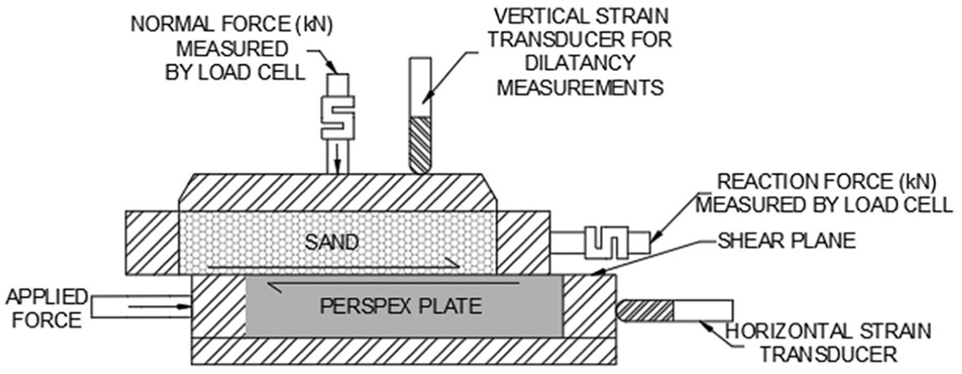
Direct shear test setup.

Input motion

The hand-held vibration analyser was used to capture the actual motion of the shake table. The maximum frequency of 100 Hz was set to capture with interval of 0.25 Hz. The final data shown by the hand-held vibration analyser are the average of data obtained by 10 cycles of shake table movement. It is assumed that the vibration captured by the hand-held vibration analyser is purely from the shake table, the cut-off frequency of input motion was set to 25 Hz for numerical analysis. The test is performed by changing the shake table displacement and its frequencies. Figure 8 shows the frequency spectrum for various motions of shake table during the test.

Figure 8.

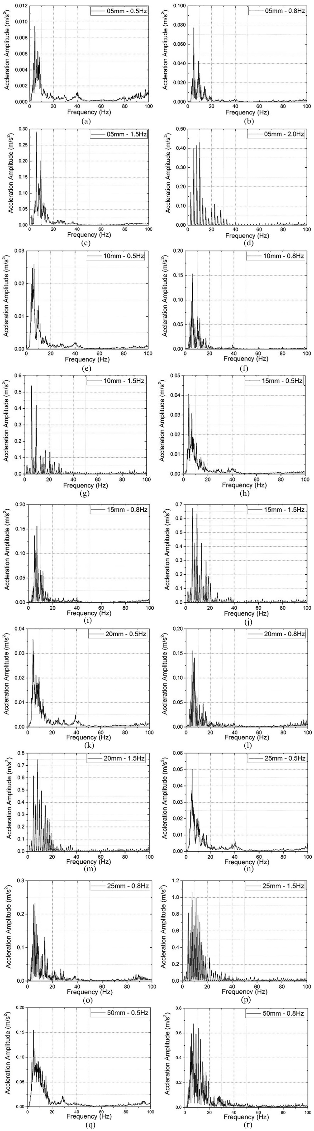
Frequency spectrum of shake table motion: (a) 5 mm – 0.5 Hz, (b) 5 mm – 0.8 Hz, (c) 5 mm – 1.5 Hz, (d) 5 mm – 2.0 Hz, (e) 10 mm – 0.5 Hz, (f) 10 mm – 0.8 Hz, (g) 10 mm – 1.5 Hz, (h) 15 mm – 0.5 Hz, (i) 15 mm – 0.8 Hz, (j) 15 mm – 1.5 Hz, (k) 20 mm – 0.5 Hz, (l) 20 mm – 0.8 Hz, (m) 20 mm – 1.5 Hz, (n) 25 mm – 0.5 Hz, (o) 25 mm – 0.8 Hz, (p) 25 mm – 1.5 Hz, (q) 50 mm – 0.5 Hz and (r) 50 mm – 0.8 Hz.

The hand-held vibration analyser captured the frequency and amplitude of shake table motion. Non-linear dynamic analysis is complex in the frequency domain. Therefore, to convert the data from frequency domain to time domain, a MATLAB code was developed. Figure 9 shows a sample for conversion from frequency domain to time domain for 50-mm displacement with 0.5 Hz frequency. In addition, the shake table motion closely simulates the actual earthquake in terms of predominant frequency. For actual earthquake, predominant frequency is near 1.5 Hz and the frequency range of shake table tests are from 0.5 to 1.5 Hz.

Figure 9.

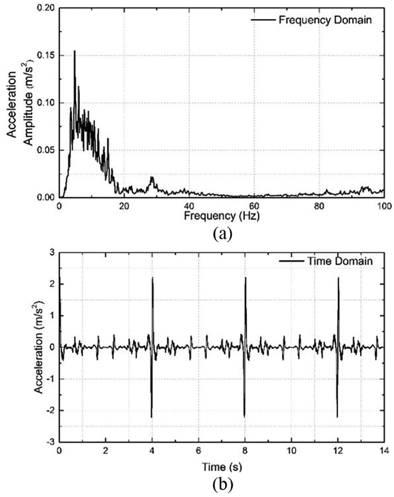
Conversion of shake table frequency domain motion into time domain motion for 50-mm displacement and 0.5-Hz frequency: (a) frequency domain and (b) time domain.

Experimental test

The soil container was firmly fixed to the shake table. The dry sandy soil was placed in container in three layers by air pluviation. Additional tamping was given to achieve the desired density (Figure 4). The tunnels were placed in the soil at the cover of 10, 30 and 50 cm, in parallel and perpendicular to the direction of shake table motion. The sensors were arranged as shown in Figures 2 and 3. The seismic force was induced by changing the displacement and frequencies as explained earlier. The dynamic soil pressure generated during each motion was captured. There were in total, 18 sets of tests for single arrangement of the tunnel and there were total 18 such arrangements (2_Orientation × 3_Cover × 3_{Different Diameter Tunnels} = 18).

Numerical modelling

The three-dimensional (3D) numerical model was prepared for tunnels placed in the transverse direction and longitudinal direction. The numerical model was made in finite-element software ABAQUS. This software is suitable and verified for use in static and dynamic analysis of underground structures.¹⁴ In 3D model, the tunnel is made with four-node shell element. Soil, foam and container are modelled with eight-node brick elements of minimum element size 0.01 m and maximum element size 0.1 m (Figure 8). The soil–tunnel interaction was modelled as coulomb friction. The slippage between soil and foam is ignored. The master–slave surfaces are used to simulate the soil–tunnel interaction with coefficient of friction as 0.12. The input motion was applied at the base of the container. The frequency dependent Rayleigh damping factors α and β were calculated by adopting the damping ratio of 5% for soil and 25% for foam. The predominant frequencies were taken by performing linear dynamic analysis on the 3D model of the tunnel.

The base motion used for numerical model is the one which was captured by the hand-held vibration analyser in frequency domain and later converted to the time domain (Figure 10). The Mohr–Coulomb material model was used for dry sand in the present analysis, and the tunnel was modelled as elastic material.

Figure 10.

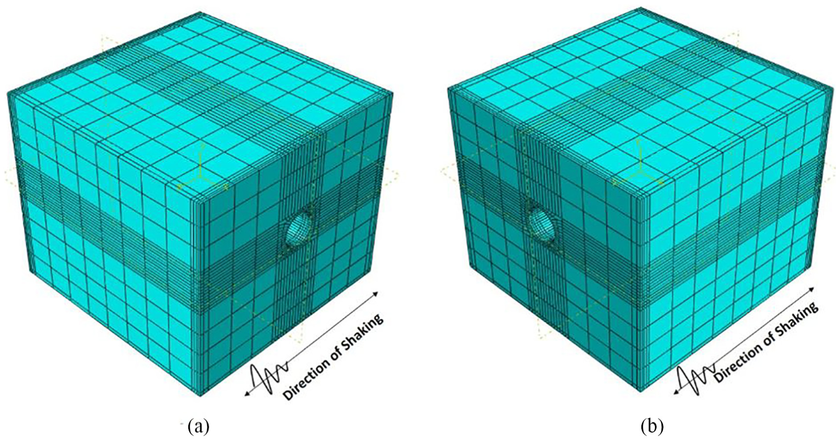
3D model of tunnel placed in (a) transverse direction and (b) longitudinal direction.

To perform an analysis close to the real state, the geostatic stress is calculated first. In this stage, the elements of the tunnel are deactivated, this produces the vertical displacement in order of 10^–6 m. In the second stage, the soil is excavated by deactivating the elements in the region of excavation, simultaneously the elements of the tunnel are activated, providing the support to the excavated soil. In the third stage, the earthquake dynamic load is applied at the base of the model. Time discretization for incremental calculation is small enough to achieve a stable and accurate solution; for present analysis, it is considered as 0.001 s. The cohesion of 1 kPa was used for sand to avoid numerical instability problems.

Results and discussion

Effectiveness of absorbing boundary

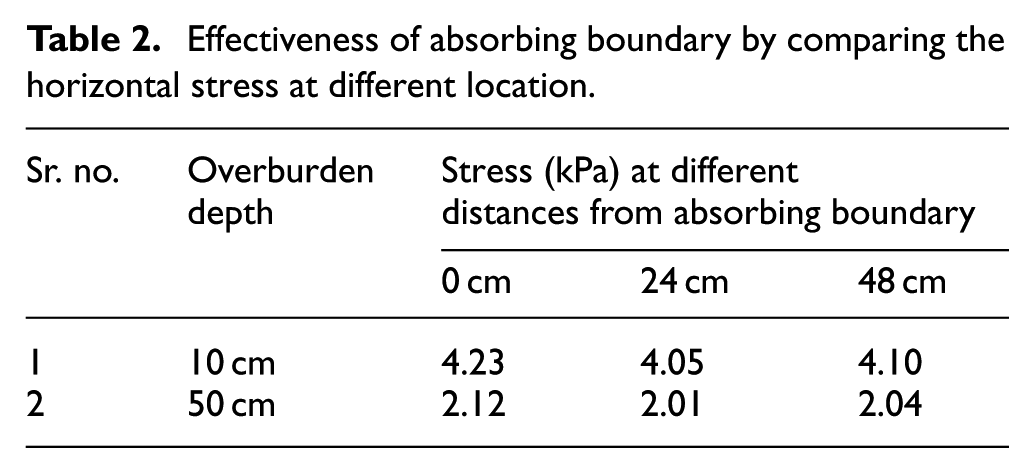
The efficiency of absorbing boundary was checked by measuring the stresses at two different elevations (at 10 and 50 cm from top) in soil without tunnel. The overall depth of sand layer was 85 cm. Three soil pressures were installed at different distances from absorbing boundary (at 0, 24 and 48 cm). Table 2 shows the results of horizontal stress in direction of shaking (25 mm displacement with 1.5 Hz frequency), recorded to check the efficiency of absorbing boundary. There is ±5% deviation in peak dynamic stress value, which is acceptable. All other shaking intensities are smaller than 25-mm displacement and 1.5-Hz frequencies, so deviation in peak dynamic stress is even smaller. For shallow cover, the horizontal dynamic stress is more than larger cover.

Table 2.

Effectiveness of absorbing boundary by comparing the horizontal stress at different location.

Sr. no.	Overburden depth	Stress (kPa) at different distances from absorbing boundary
		0 cm	24 cm	48 cm
1	10 cm	4.23	4.05	4.10
2	50 cm	2.12	2.01	2.04

Rigidity of soil container

In the experimental work and numerical analysis, the soil container was assumed to be rigid. For present numerical simulation acceleration response of soil container was checked at two locations (Figure 11). One location where hand-held vibration analyser is attached (Figure 2) and other location is directly opposite to it. In addition, the data recorded from hand-held vibration analyser is shown in Figure 11. The acceleration response of numerical simulation for soil containers at two locations (middle section of right and left vertical wall) and from experimental work is matched. This shows that the soil container is rigid as the phase lag of acceleration response between two vertical walls is negligible.

Figure 11.

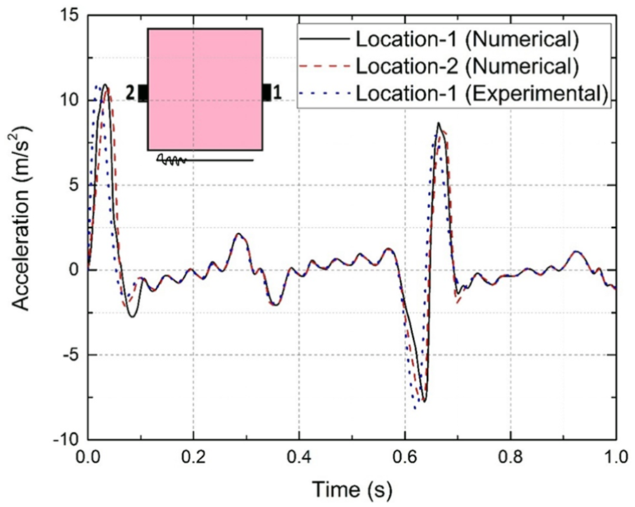
Acceleration response of soil container for shake table displacement of 25 mm and frequency 1.5 Hz.

Flexibility ratio of tunnel

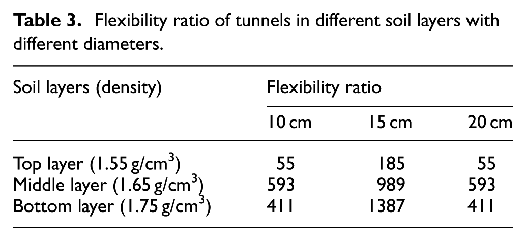
To determine the relative stiffness between a circular tunnel lining and the soil medium, the flexibility ratio is defined by equation (5). Flexibility ratio measures the ability of the tunnel to resist the distortion imposed from soil medium during seismic load.

\begin{matrix} Flexibility ratio = \frac{E_{s} (1 - ν_{t}^{2}) R^{3}}{6 E_{t} I (1 + ν_{m})} \end{matrix}

(5)

where E_s is the modulus of elasticity of the medium, ν_m is Poisson’s ratio of the medium, E_t is the modulus of elasticity of the tunnel lining, ν_t is Poisson’s ratio of the tunnel, R is the radius of the tunnel lining, t is the thickness of the tunnel lining and I is the moment of inertia of the tunnel lining (per unit width). Table 3 shows the flexibility ratio of three different diameters of the tunnel. The flexibility ratio is calculated for tunnel placed in three different layers. Wide variety of flexibility ratio of tunnel was used for present test. However, the flexibility ratio shown is valid for tunnel embedded in single layer. Tunnel embedded in two layers may have different flexibility ratio.

Table 3.

Flexibility ratio of tunnels in different soil layers with different diameters.

Soil layers (density)	Flexibility ratio
	10 cm	15 cm	20 cm
Top layer (1.55 g/cm³)	55	185	55
Middle layer (1.65 g/cm³)	593	989	593
Bottom layer (1.75 g/cm³)	411	1387	411

Peak dynamic stresses from experiment and numerical model

The results from the shake table experiment and numerical modelling are represented in the form of graphs. The stresses are expressed in percentage increase of peak dynamic stresses with respect to the corresponding value of stress generated during static analysis. The percentage change in peak dynamic stresses is plotted against the input motion of shake table (displacement (mm) – frequency (Hz)). Some discrepancies may come due to recording issues that are present in soil pressure transducers.¹³ In addition, the relative stiffness of sensing plate and effect of grain size distribution may affect the results.²⁰ In general, peak dynamic stresses from numerical analysis are in good agreement with the experimental results. However, slight difference in results from experiments and numerical model is observed for 10 cm cover.

Tunnel in longitudinal direction

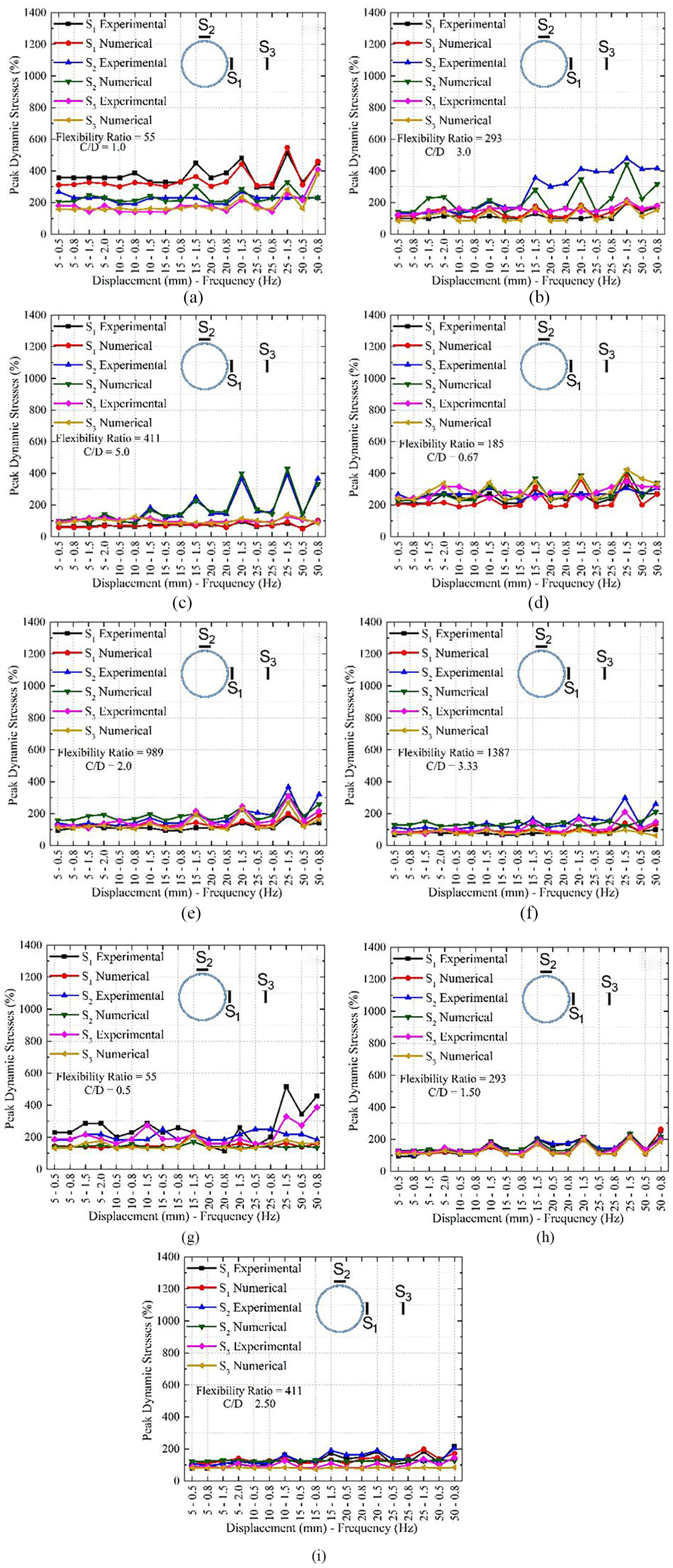
Figure 12 shows the percentage increase in peak dynamic stresses for different diameters of tunnel at different cover. The tunnel is placed in longitudinal direction. Flexible tunnel generates less dynamic stresses. Increase in cover-to-diameter (C/D) ratio decreases the dynamic stresses. Large diameter tunnels are subjected to less dynamic stresses with the same flexibility ratio at same cover.

Figure 12.

Peak dynamic stresses in fine sandy soil for tunnel in longitudinal direction: (a) T_10/10, (b) T_10/30, (c) T_10/50, (d) T_15/10, (e) T_15/30, (f) T_15/50, (g) T_20/10, (h) T_20/30 and (i) T_20/50.

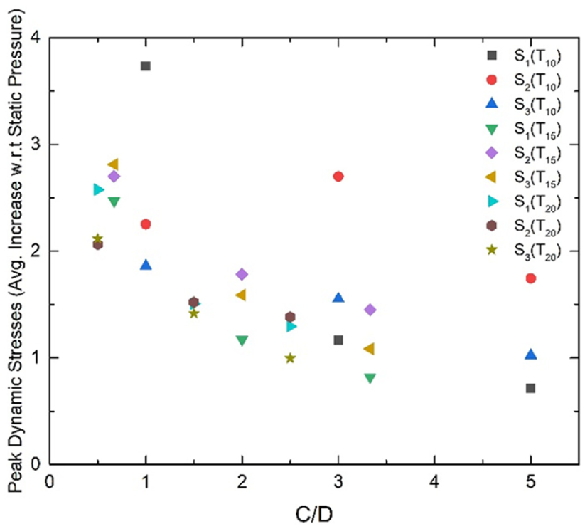
Figure 13 shows the average increase in peak dynamic stresses with respect to static pressure versus C/D ratio for tunnel in longitudinal direction. It was observed that vertical dynamic stresses are predominant. For C/D <3.0 S₁ is more than S₃. Tunnel in longitudinal direction shows, rocking behaviour of the tunnel, and it increases with an increase in intensity of shaking.

Figure 13.

Average increase in peak dynamic stresses with respect to static pressure versus C/D ratio for tunnel in longitudinal direction.

Tunnel in transverse direction

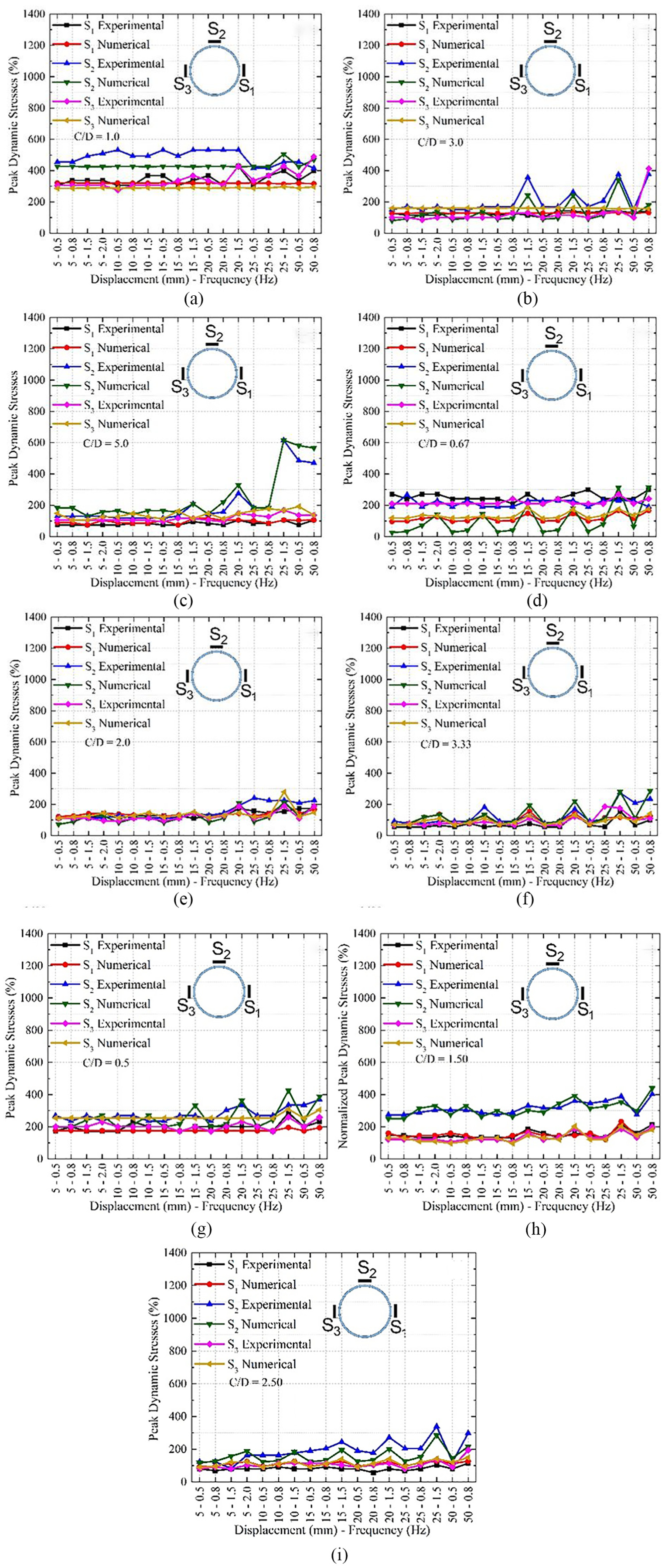
Figure 14 shows the percentage increase in peak dynamic stresses for different diameters of tunnel at different cover. The tunnel is placed in transverse direction. The abscissa represents various loading conditions, whereas ordinate shows the normalized peak dynamic stresses value. It was observed that tunnel with same flexibility ratios (T₁₀ and T₂₀), smaller diameter tunnel generates more stresses, about three to four times higher. With the increase in C/D ratio, the dynamic stresses decrease. In addition, increase in flexibility ratio decreases the peak dynamic stress. T₁₀ shows significant increase in vertical dynamic stresses at a frequency of 1.5 Hz.

Figure 14.

Peak dynamic stresses in fine sandy soil for tunnel in transverse direction: (a) T_10/10, (b) T_10/30, (c) T_10/50, (d) T_15/10, (e) T_15/30, (f) T_15/50, (g) T_20/10, (h) T_20/30 and (i) T_20/50.

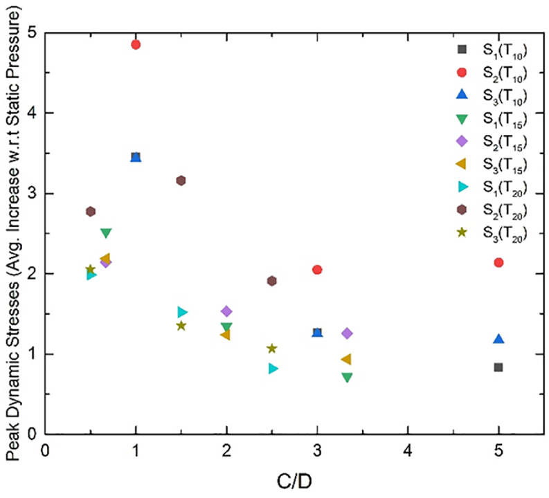
Figure 15 shows the average increase in peak dynamic stresses with respect to static pressure versus C/D ratio for tunnel in transverse direction. Vertical stresses are predominant for smaller diameter of the tunnel (T₁₀) and at shallow depth. In addition, with an increase in depth, vertical stresses are becoming predominant. For less flexible tunnel (T₁₀ and T₂₀) S₁ is greater than S₃.

Figure 15.

Average increase in peak dynamic stresses with respect to static pressure versus C/D ratio for tunnel in transverse direction.

Soil pressure transducer response

Figures 16 –19 shows the plots of dynamic stresses from experiment and numerical analysis for 15cm tunnel diameter, 30 cm cover and input motion of ±25 mm displacement and 1.5 Hz frequency. This is the strongest input motion generated from the shake table for present test and this is the reason for its selection. The time history results are compared for tunnel in longitudinal (Figure 16) and transverse (Figure 17) direction. In addition, the results are compared in terms of FFT for tunnel in longitudinal (Figure 18) and transverse (Figure 19) direction. The comparison shows that numerical predictions are in the same order of magnitude with the experimental results. The difference recognized is due to the small settlement of 3 mm occurs during the dynamic analysis step in numerical modelling. However, the proposed model captures peak dynamic stresses well. And the design of civil engineering structures is based on the peak stresses.

Figure 16.

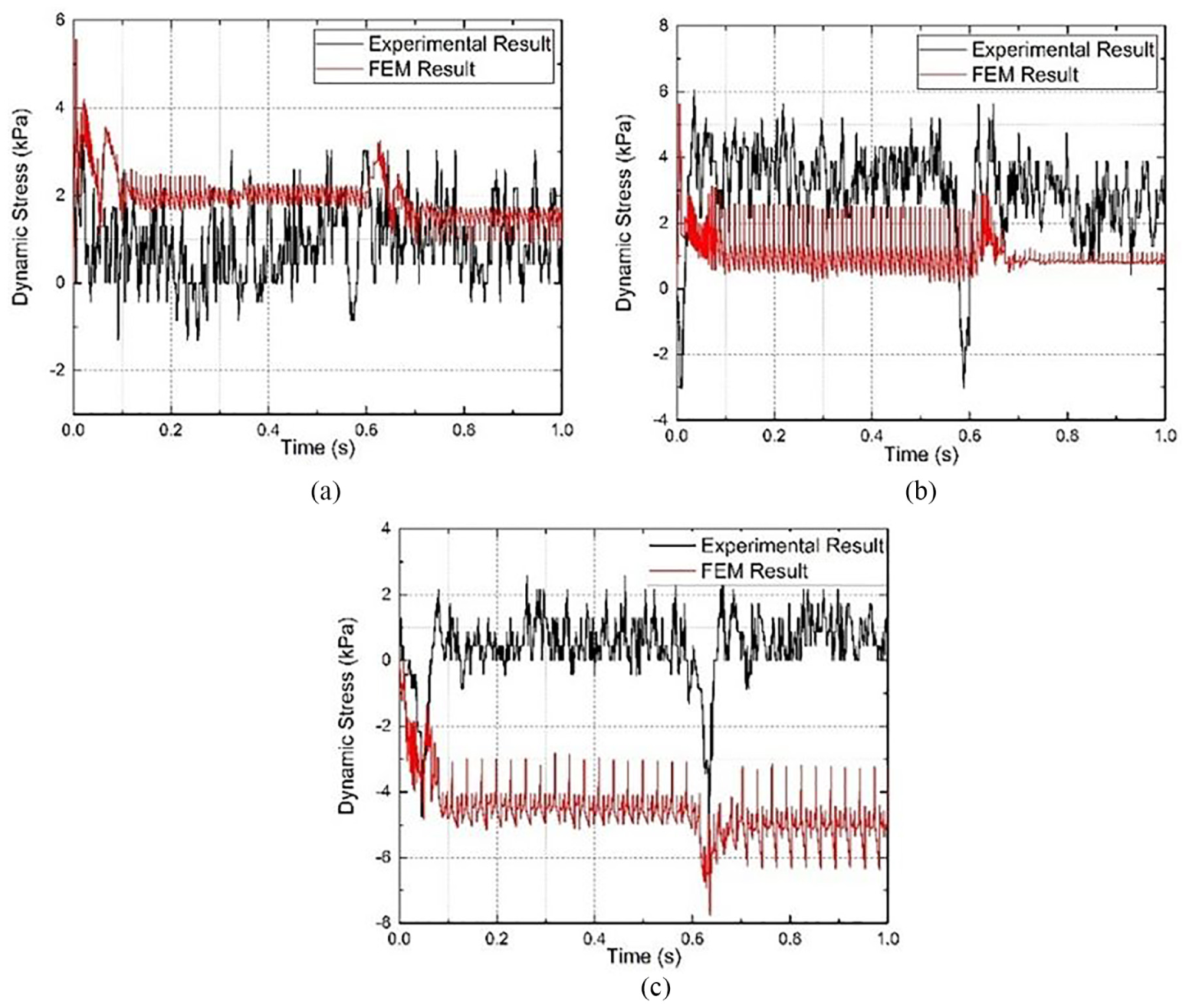
Time versus dynamic stresses for tunnel in longitudinal direction having diameter 15 cm and overburden depth as 30 cm: (a) Sensor S₁, (b) Sensor S₂ and (c) Sensor S₃.

Figure 17.

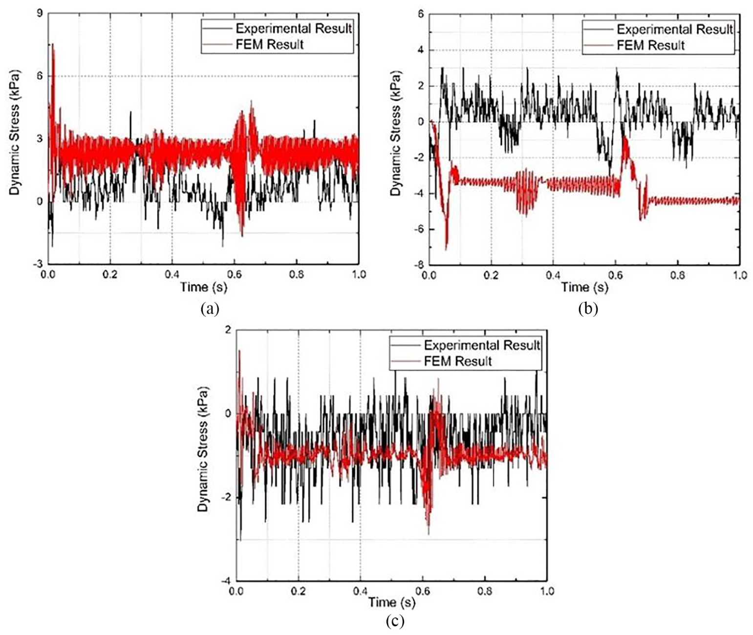
Time versus dynamic stresses for tunnel transverse direction having diameter 15 cm and overburden depth as 30 cm: (a) Sensor S₁, (b) Sensor S₂ and (c) Sensor S₃.

Figure 18.

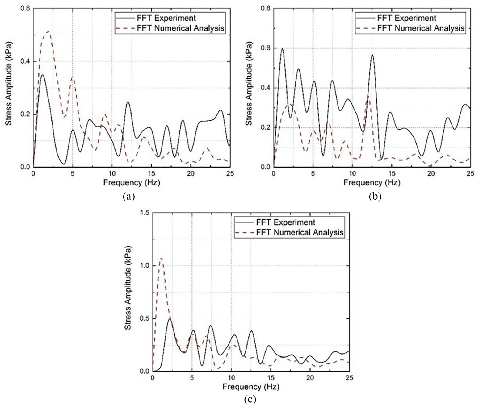
Frequency versus dynamic stresses for tunnel longitudinal direction having diameter 15 cm and overburden depth as 30 cm: (a) Sensor S₁, (b) Sensor S₂ and (c) Sensor S₃.

Figure 19.

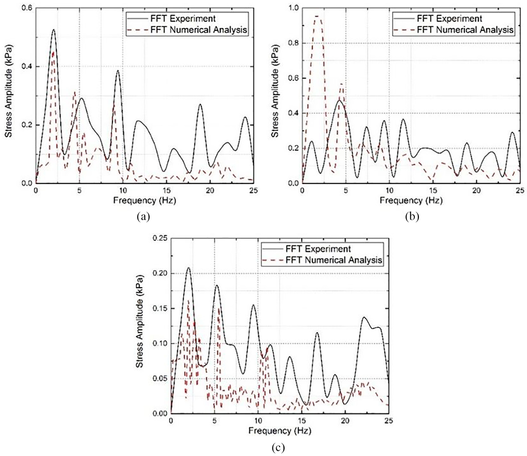
Frequency versus dynamic stresses for tunnel transverse direction having diameter 15 cm and overburden depth as 30 cm: (a) Sensor S₁, (b) Sensor S₂ and (c) Sensor S₃.

Tunnel design guidelines

Most codes follow a dual-design philosophy for earthquake-resistant design of buildings. First is a design-based earthquake (DBE), which is expected to occur during the design life of the building. In such earthquakes, the structure should get only minor or moderate damage. Second is maximum considered earthquake (MCE), which is expected that the structural damage should not result in total collapse.

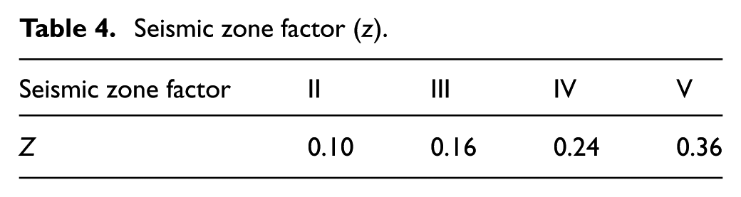
According IS 1893:2016, India is divided into four zones (zone-II, -III, -IV and -V) of the earthquake. Zone-II is associated with the lowest level of seismicity, whereas Zone-V expects the highest level of seismicity.²¹ The zone factors used in the design of civil engineering is 0.10g, 0.16g, 0.24g and 0.36g for zone-II, -III, -IV and –V, respectively. These zone factors are based on PGA of an MCE. Furthermore, these zones are created based on Medvedev–Sponheuer–Karnik (MSK) intensity scale, where zone-V corresponds to intensity above IX. Rupture in underground pipeline can be observed at this intensity. However, there are no special provisions for design of underground structures in Indian code as well as in national codes of other countries.

IS 4880:Part-5 states that if seismic force is significant, it should be considered in the design. In addition, for extreme loading condition, the stresses on the tunnel lining from the soil is to be increased by 33.3%.²² Seismic force should be considered for the underground utilities tunnel if design earthquake spectral response acceleration of a site is more than 0.33.²³ However, the response of tunnel greatly depends on the surrounding soil, C/D ratio and the flexibility ratio of tunnel.

In the present shake table tests, total 18 different ground motions were used with a wide variety of PGA motion (0.01g–1.20g). Zone-II and zone-V have six motions each, whereas zone-III and zone-IV have three motions each (Figure 20).

Figure 20.

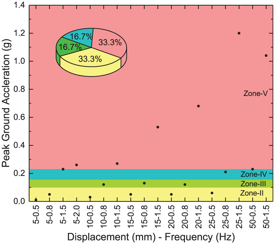
Input motion versus peak ground acceleration (zones are as per Indian Standard 1893:2016).

Design steps

Get the seismic zone factor as per IS 1893: 2016 (Table 4).

Select the stress amplification coefficient (Table 5).

Use the equation (6) to calculate the maximum dynamic soil pressure

\begin{matrix} S_{dyn (MCE)} = \frac{z}{K} S_{static} \end{matrix}

(6)

Table 4.

Seismic zone factor (z).

Seismic zone factor	II	III	IV	V
Z	0.10	0.16	0.24	0.36

Table 5.

Design coefficient (K).

C/D	Z-II	Z-III	Z-IV	Z-V
0.5–1	0.04	0.06	0.09	0.12
1–3	0.07	0.11	0.16	0.18
3–5	0.11	0.17	0.21	0.22

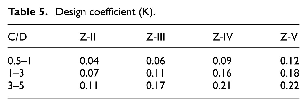
where S_dyn_(MCE) is the peak dynamic pressure for MCE, z is the zone factor, K is the stress amplification coefficient, and S_static is the static pressure on the tunnel.

4. Use the equation (7) to calculate the design-based maximum dynamic soil pressure

\begin{matrix} S_{dyn (DBE)} = \frac{2}{3} S_{dyn (MCE)} \end{matrix}

(7)

Equation (7) should be used to get the value for peak vertical as well as peak horizontal dynamic pressure. The value calculated from equation (7) is in addition to static soil pressure.

Conclusion

A study of seismic response of a circular tunnel was made using shake table testing and finite-element numerical modelling. The compaction of sand was carried out to maximum possible densities along the depth, to avoid settlement during shaking. The bender element test is used to get mechanical properties of materials. The numerical results were compared with experimental measurements in terms of peak dynamic stresses. The comparison shows the numerical results are in good agreement with the test results.

The civil engineering structures are designed against the peak stresses and in case of flexible tunnel peak horizontal stresses in soil near tunnel face are less than the stresses observed at some distance from the tunnel. Overall, there is a reduction of peak dynamic stresses in soil as the flexibility of tunnel increases. In addition, with increase in C/D ratio, the peak dynamic stresses decrease by significantly. Tunnel with smaller diameter generates larger peak dynamic stresses in soil less as compared to the larger diameter tunnel at the same C/D ratio and flexibility ratio. Therefore, it is better to have a flexible support to reduce the impact of such forces. It is also observed that, while designing the tunnel, peak vertical stresses also need to be considered, as they are predominant at higher frequencies, especially when the tunnel is placed in longitudinal direction of shaking.

Footnotes

Appendix 1 Acknowledgements

The authors wish to acknowledge the Department of Science and Technology – SERB (grant no.: SB/S3/CEE/0002/2013) for providing the financial support to carry out this research work.

Declaration of conflicting interests

The author(s) declared no potential conflicts of interest with respect to the research, authorship, and/or publication of this article.

Funding

The author(s) received no financial support for the research, authorship, and/or publication of this article.

ORCID iD

DK Singh

References

Yashiro

Kojima

Shimizu

Historical earthquake damage to tunnels in Japan and case studies of railway tunnels in the 2004 Niigataken-Chuetsu earthquake. Q Rep RTRI 2007; 48: 136–141.

Wang

Seismic design of tunnels: a simple state-of-the-art design approach. New York: Parsons Brinckerhoff, 1993.

Clark

Practice of dynamic pressure measurement. Meas Control 1989; 22: 298–301.

White

GWT

. Methods of modelling and simulating dynamic systems. Meas Control 1971; 4: T139–T146.

Lanzano

Bilotta

Russo

, et al. Experimental and numerical study on circular tunnels under seismic loading. Eur J Environ Civ Eng 2015; 19: 539–563.

Chen

Jiang

, et al. Numerical simulation of shaking table test on utility tunnel under non-uniform earthquake excitation. Tunn Undergr Sp Technol 2012; 30: 205–216.

Chen

Shi

Shaking table test of utility tunnel under non-uniform earthquake wave excitation. Soil Dyn Earthq Eng 2010; 30: 1400–1416.

Ling

Mohri

Kawabata

, et al. Centrifugal modeling of seismic behavior of large-diameter pipe in liquefiable soil. J Geotech Geoenviron Eng 2003; 129: 1092–1101.

Pitilakis

Dietz

Wood

, et al. Numerical simulation of dynamic soil–structure interaction in shaking table testing. Soil Dyn Earthq Eng 2008; 28: 453–467.

10.

Cilingir

Gopal Madabhushi

SP.

A model study on the effects of input motion on the seismic behaviour of tunnels. Soil Dyn Earthq Eng 2011; 31: 452–462.

11.

Cilingir

Madabhushi

SPG

. Effect of depth on seismic response of circular tunnels. Can Geotech J 2011; 48: 117–127.

12.

Buonsanti

Leonardi

3-D simulation of tunnel structures under blast loading. Arch Civ Mech Eng 2013; 13: 128–134.

13.

Tsinidis

Pitilakis

Madabhushi

, et al. Dynamic response of flexible square tunnels: centrifuge testing and validation of existing design methodologies. Géotechnique 2015; 65: 401–417.

14.

Huo

Bobet

Fernández

, et al. Load transfer mechanisms between underground structure and surrounding ground: evaluation of the failure of the Daikai station. J Geotech Geoenviron Eng 2005; 131: 1522–1533.

15.

Penzien

Seismically induced racking of tunnel linings. Earthq Eng Struct Dyn 2000; 29: 683–691.

16.

Lombardi

Bhattacharya

Scarpa

, et al. Dynamic response of a geotechnical rigid model container with absorbing boundaries. Soil Dyn Earthq Eng 2015; 69: 46–56.

17.

ASTM D3574-17. Standard test methods for flexible cellular materials – slab, bonded, and molded urethane foams. West Conshohocken, PA: ASTM International.

18.

Camacho-Tauta

Álvarez-Jiménez

Reyes-Ortiz

OJ.

A procedure to calibrate and perform the bender element test. Dyna 2012; 79: 10–18.

19.

Kataoka

Kawaguchi

Horita

. Unconfined compression strength and elastic shear modulus of air-form treated lightweight soil. In: Proceedings of the 5th international symposium on deformation characteristics of geomaterials, Seoul, South Korea, 1–3 September 2011, pp. 682–686. Amsterdam: IOS Press.

20.

Cilingir

Seismic response of tunnels. Cambridge: Geotechnical Engineering Group, 2009.

21.

IS 1893 Part-1. Criteria for earthquake resistant design of structures, part-1 general provisions, and buildings. New Delhi, India: Bureau of Indian Standard, 2016.

22.

IS 4480 Part-5. Code of practice for design of tunnels conveying water, part v structural design of concrete lining in soft strata and soils. New Delhi, India: Bureau of Indian Standard, 2000.

23.

ASCE/SEI 7-16. Minimum design loads for buildings and other structures. Reston, VA: American Society of Civil Engineers, 1994.

Effect of earthquake excitation on circular tunnels: Numerical and experimental study

Abstract

Keywords

Introduction

Experimental setup

Shake table

Soil container/tank

Sensors setup

Methodology

Soil filling in container/tank

Absorbing boundary

Material properties

Input motion

Experimental test

Numerical modelling

Results and discussion

Effectiveness of absorbing boundary

Rigidity of soil container

Flexibility ratio of tunnel

Peak dynamic stresses from experiment and numerical model

Tunnel in longitudinal direction

Tunnel in transverse direction

Soil pressure transducer response

Tunnel design guidelines

Design steps

Conclusion

Footnotes

Appendix 1

Acknowledgements

Declaration of conflicting interests

Funding

ORCID iD

References