
Abstract
Most dynamic systems in practice are of fractional order and often the models using fractional-order equations can grasp their intrinsic properties with more accuracy compared with conventional differential equations. In this paper, a fractional-order modeling-based proportional–integral–derivative-type dynamic matrix control is developed and tested on a typical industrial heating furnace system with fractional-order dynamics. The Oustaloup approximation method is first adopted to obtain the model approximation of the processes, which paves the way for the application of integer order dynamic matrix control to the fractional-order systems. Meanwhile, a set of proportional–integral–derivative-type operators are introduced in the cost function to further optimize the dynamic matrix control in terms of tracking and disturbance-rejection performance. The resulting controller bears both the merits of the dynamic matrix control and the proportional–integral–derivative, and thus improved control performance is obtained. In addition, an industrial heating furnace process system is given to test the performance of the proposed method in comparison with traditional integer order model-based dynamic matrix control, and results show that the proposed method gives improved system performance.
Keywords
Introduction
For industrial processes, proportional–integral–derivative (PID) control and model predictive control (MPC) are the most widely used control technologies and a lot of progress has been achieved. Dynamic matrix control (DMC) is a typical MPC that was first proposed by Culter et al. 1 in 1980. It extends the single-step prediction of traditional self-tuning technology to the multi-step prediction and carries out the receding horizon optimization, such that the sensitivity to the variation of model parameters is effectively restrained, and the effects of the uncertainty factors such as environmental interference and modeling error are reduced.2,3 DMC is effective in the control applications of industrial processes with strong coupling, nonlinearity, large time delay, and so on.4–6 However, DMC is usually designed on the basis of the asymptotically stable linear approximated model, which may require larger online computation, leading to the fact that the disturbance cannot be restrained quickly. Therefore, it is meaningful to study the improvement of DMC algorithm for the control systems under various uncertainties. 7
The traditional PID control is a feedback control that is composed of three linear combinations of the feedback of system error. It is still widely used in industrial processes due to its merits of simple structure and strong robustness. However, with regard to the situation that the parameters of the process model are of nonlinearity, time varying uncertainty, and large inertia or time delay under the uncertain disturbance, it is not easy for conventional PID control to achieve the desired control effect.8,9 In this regard, some methods were put forward to improve the control performance, for example, the cascade control of superheated steam temperature, such as DMC-PID which is also called predictive PID controller. 10 In this strategy, the weighted term of the steady-state error was introduced into the cost function of generalized predictive control (GPC), and the control law was established again based on the PID structure. The algorithm was decomposed according to the PID form, and a PID controller with prediction function was finally obtained. The advantages of PID and DMC control were further reported in Yao and Guo, 11 where the cost function of DMC was established again in the form of PID, and a new predictive control method was obtained. Moreover, the PID-type DMC (PIDDMC) algorithm is further extended to multivariable system in order to overcome the shortcoming of not optimizing system performance. 12
The application of PID control and DMC in practice are based on process modeling and the control performance will be greatly influenced by the modeling accuracy. 13 Modeling is an important component of the dynamic system control theory.14,15 The integer order model-based control theory is now mature and widely used. In practice, most of the dynamic systems are of fractional order and the integer order differential equation model will only describe part of the dynamic characteristics of such systems. Thus, research on extending the control method of the integer order model-based control theory to fractional-order systems is a meaningful job. In the literature,16–18 different fractional-order models described by the differential equation, the state space model, the transfer function model, the fractional difference equation, and the fractional-order discretization are discussed and studied, and detailed description about mutual transformation among the models are also given.
The number of arbitrary orders and the distinctive memory feature of fractional-order calculus can reflect the inherent characteristics of these systems more precisely. A fractional-order controller is a controller in which the fractional calculus operator is introduced and utilized. Among the fractional-order model-based control, the
Existing research focusing on the fractional-order model-based controller design has been reported in Özbay et al. 25 Rhouma et al.26,27 proposed a MPC for fractional-order systems in which the numerical and Oustaloup approximation were used for output prediction. The fractional-order implementation method and the application of a novel predictive controller RTD-A was studied in Li et al. 28 Ji and Li 29 proposed the design and implementation of MPC based on the fractional Kalman filter, and the estimated state was used for MPC. Vmager et al. 30 studied a fractional-order model reference adaptive control scheme that improves the dynamic closed-loop system performance. Romero et al.31,32 proposed a GPC method for fractional-order systems by introducing the fractional-order operator, which was introduced into the cost function. Deng et al. 33 proposed an adaptive GPC for solid oxide fuel cells with fractional-order dynamics.
As mentioned above that there are limited research results of MPC for fractional-order systems. Also, the control performance still needs to be further improved since fractional-order model-based control is not mature. Thus, a PIDDMC approach is proposed using fractional-order linear system theory. First, the Oustaloup approximation method is utilized to formulate the approximated model of fractional-order systems. Second, a PID-type operator is introduced into the controller design that will make the adjustment of subsequent control parameters more flexible. Finally, the fractional-order DMC is derived using fractional calculus.
The reminder of the paper is as follows. In section “Theory of fractional calculus,” the theory of fractional calculus is provided, and the specific forms of the definitions of three kinds of fractional calculus are given. The design procedure of PIDDMC (fractional-order PIDDMC (FO-PIDDMC)) is presented in section “FO-PIDDMC.” We first use the Oustaloup approximation method to obtain the higher-order integer order model. Then, DMC is extended to the control of the fractional-order system, where the PID operator is introduced into the controller design. As a result, the optimal control law will be obtained. In section “Case study,” the performance of the FO-PIDDMC is verified by simulation on the temperature control of a heating furnace. Results show that the proposed controller will improve the control performance compared with traditional integer order model-based DMC. Finally, conclusion is summarized in section “Conclusion.”
Theory of fractional calculus
Fractional calculus, which is also known as the generalized calculus, is an extension of the traditional calculus, that is to say, the derivative of the function in the differential equation can be chosen as a fraction instead of an integer. As a matter of fact, it is non-integer or of any order, and the order can be both real or plural. Based on fractional calculus theory, the most three common definitions are Grünwald–Letnikov (GL), Riemann–Liouville (RL), and Caputo. 34 The mathematicians give several different definitions of fractional calculus from different points of view respectively, and the rationality of the definition has been verified in practice. Next, the three kinds of specific forms of fractional calculus definition will be given below.
GL fractional calculus definition
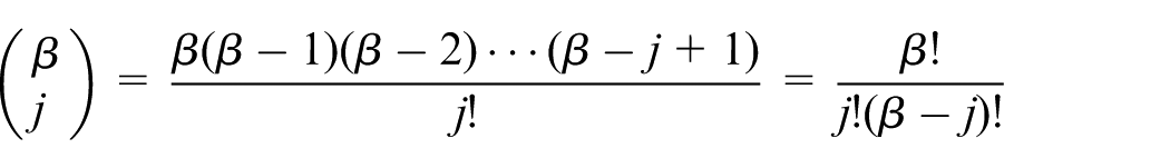
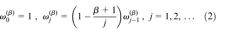
The numerical algorithm of fractional derivative can be directly derived using GL definition, which is widely used in the fractional-order control, and the specific form is described as follows
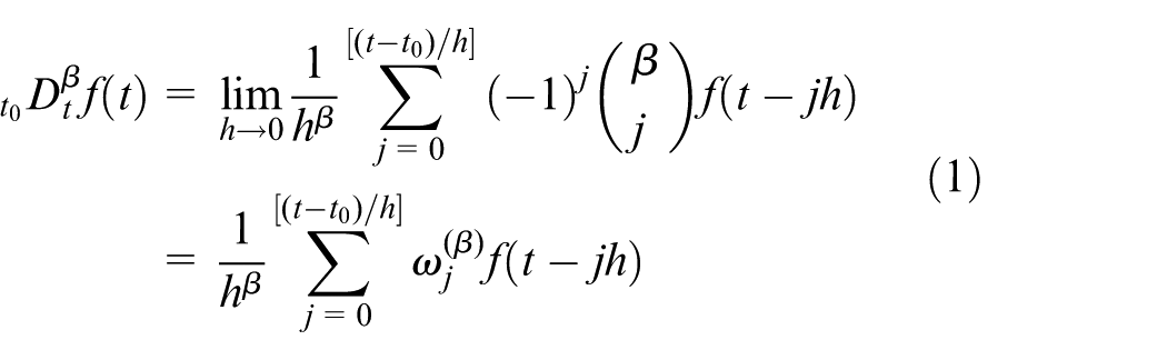
where
When application in the practical process is considered, the sampling time
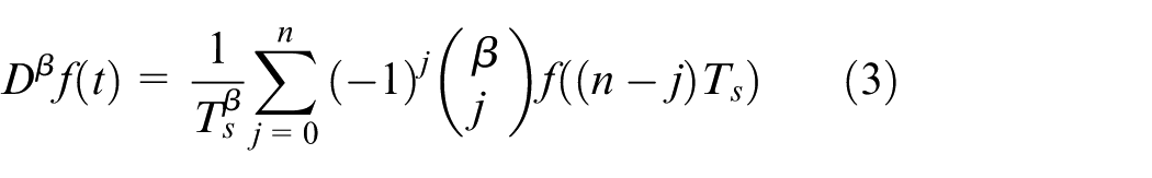
where
RL fractional calculus definition
RL definition is defined as follows
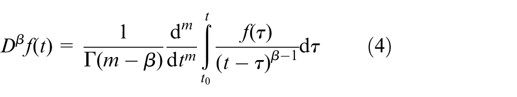
where
The Laplace transform of RL is
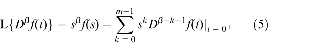
The transformation results for the initial condition are given as

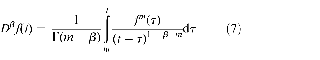
Caputo fractional calculus definition
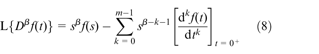
Caputo fractional calculus is
and the Laplace transform is
Representation of fractional-order systems
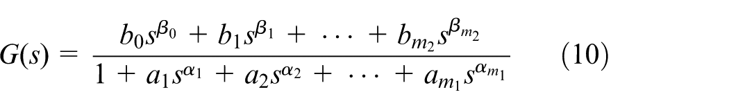
For simplicity, the typical single input single output (SISO) linear systems is considered here, and the differential equation form can be described as
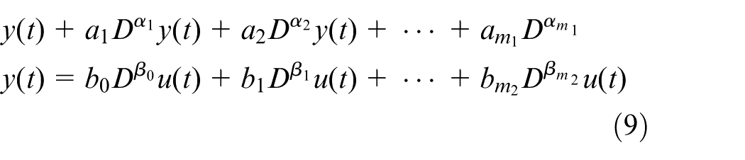
where
Note that here RL definition is used and combining with the RL definition and Equation (6), the fractional-order system with zero initial condition is written as follows
FO-PIDDMC
Model development
It is not easy to directly derive the algorithm for fractional-order systems due to the fact that controller designs are just applicable for integer order systems. Considering this fact, the Oustaloup approximation method 35 is adopted here for numerical solution of fractional-order differential equations, which is
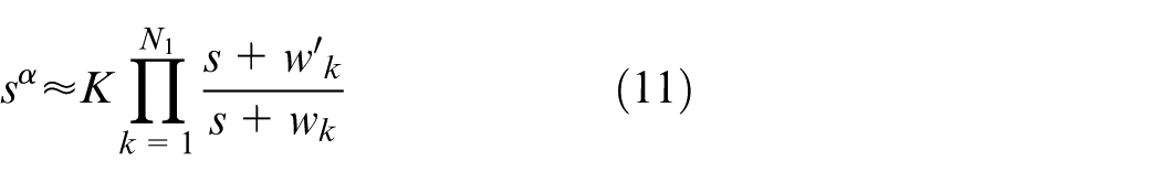
where
By using the Oustaloup approximation method, Equation (11) is substituted into the fractional-order systems in Equation (10), and the higher-order approximation of an integer order system model can be obtained. The higher-order model with the zero-order holder are discretized using the sampling time and the following is obtained
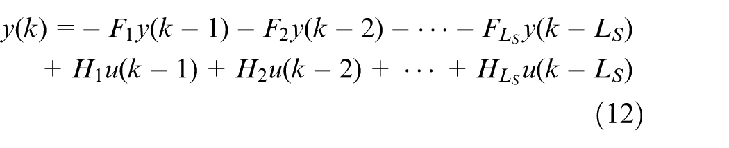
where
Design of the FO-PIDDMC controller
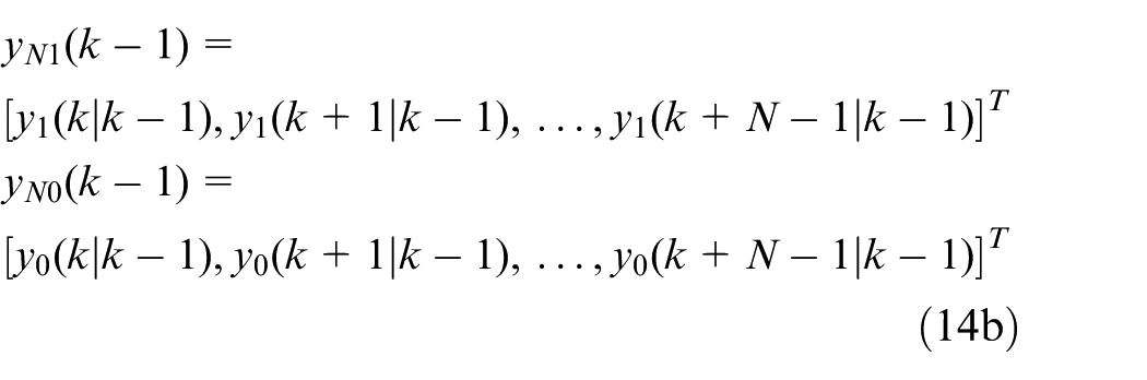
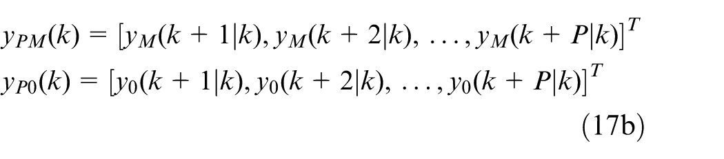
The model vector
where
The predicted output value is obtained by adding

where
It needs to modify the output prediction because of the output prediction error caused by the uncertainty of the model, which is done as follows

where
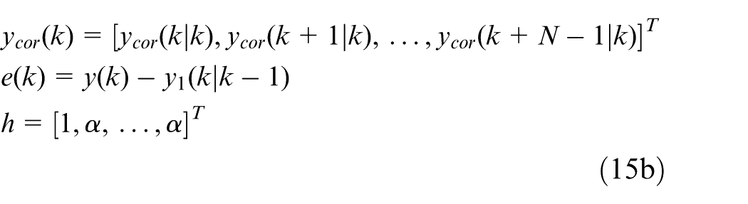
Here,
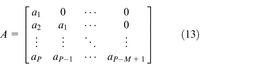
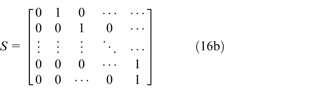
It is required to shift the elements of

where
Due to the existence of model truncation,
Furthermore,

where
Here,
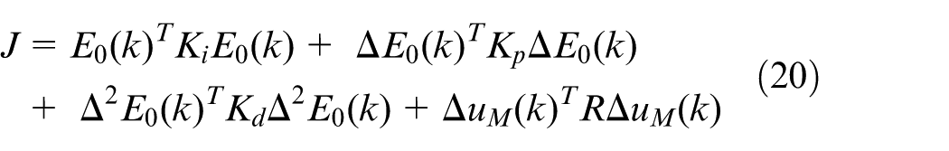
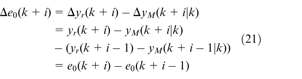
The reference trajectory and the cost function of the fractional-order DMC is selected as follows
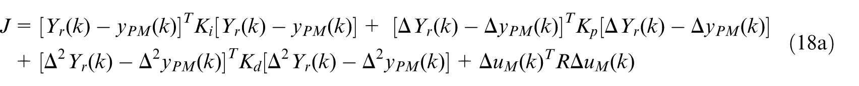

where
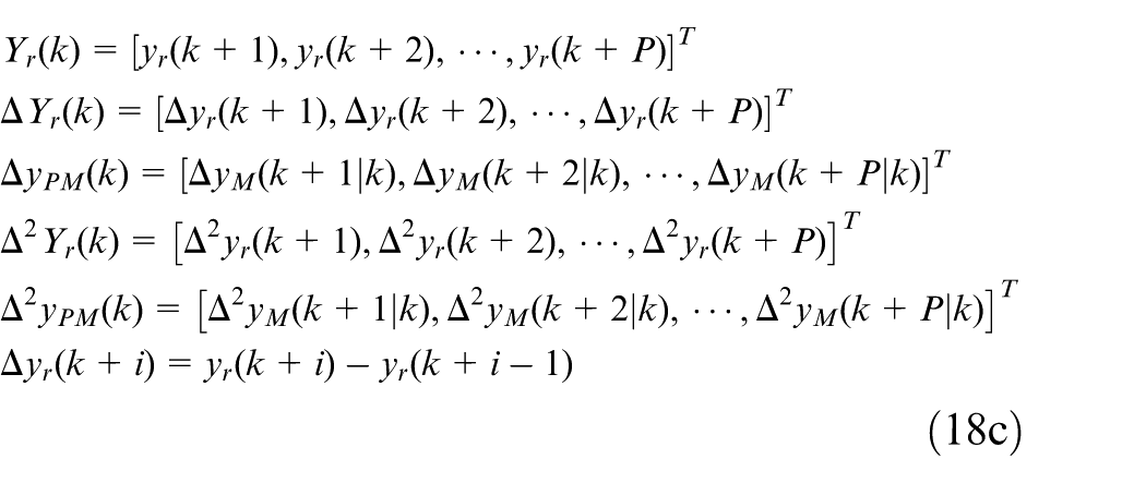


Here,
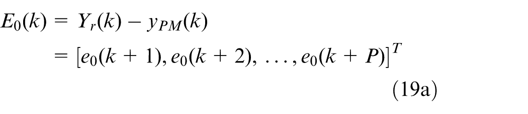
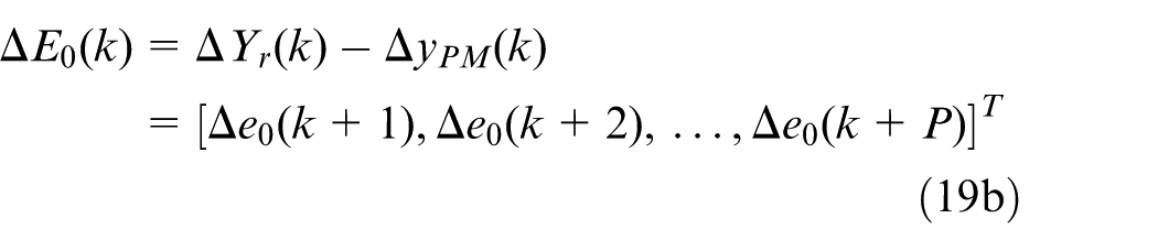
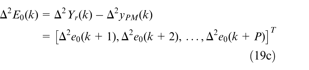
By substituting Equation (19a)–(19c) into Equation (18a), the cost function is transformed as
Combining Equations (18c), (18d), and (19b) with Equation (19c), we can obtain
In the same way

For convenience, we specifically define
By introducing a matrix
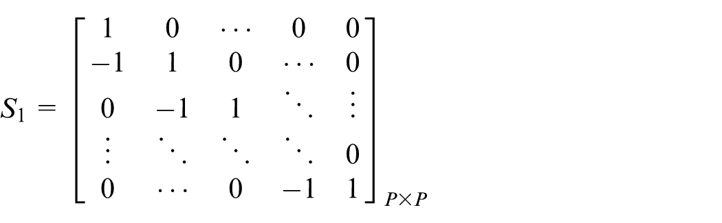
we can obtain
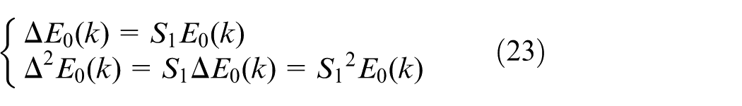
Substituting Equation (23) into Equation (20), the cost function is further transformed into the following form
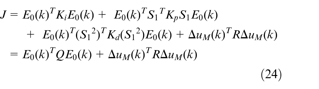
where
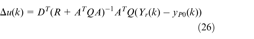
By using

Defining
Case study
The proposed FO-PIDDMC is tested on the temperature model of a heating furnace. Figure 1 displays the process flow of the heating furnace (SXF-4-10). The temperature of the heating furnace is detected by K type thermocouple and converted to a voltage signal. The voltage signal will be amplified by the signal amplifier (SG-3011 CR) and sent to the signal acquisition card (CR PCI-1802LU) and converted to the corresponding temperature value in the computer. The digital signal 0 × 01 from the computer to the signal output card (PIO-D24U) will be transformed into a voltage of +5 V for heating, which is done by sending it from the cable (DN-3710 CR) to the solid state relay (SSR-380D40). When the digital signal from the computer is 0 × 00, the corresponding voltage is 0 V and the furnace is disconnected.
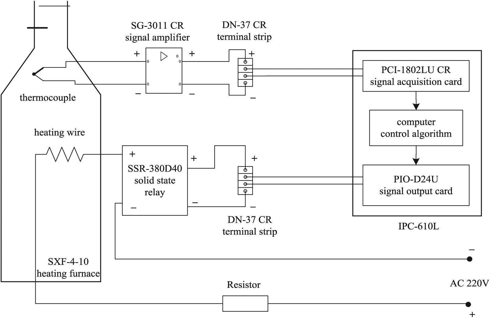
The temperature control system of high temperature resistance furnace (SXF-4-10).
Modeling
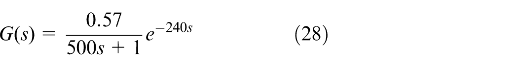
By collecting the real-time temperature data of the heating furnace, the fractional-order model and the integer model of the heating furnace can be obtained. Here, the integer model is a first-order-plus-dead-time model using the standard step response method described in Zhang and Wang 36 and as the integer model has modeled the process with a certain degree of accuracy, the fractional-order model is further obtained based on the integer model with trial and error. The two obtained models are as follows
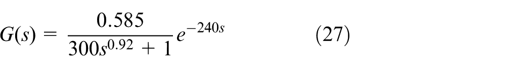
The fractional-order model Equation (27) is further treated into the higher-order model by Oustaloup method

where the approximation order is selected as N = 4, and the fitting frequencies of the Oustaloup approximation are
The output values of the three models are compared with the temperature process data and shown in Figure 2 and Table 1.
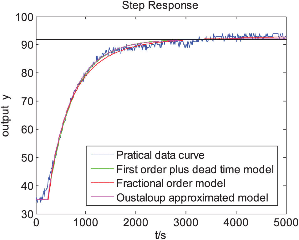
The output contrast curve of model step response.
Comparison results of the output values of the three models.
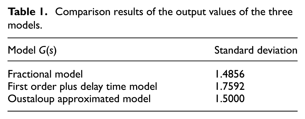
From Figure 2 and Table 1, we can find that the modeling error of the first-order-plus-dead-time model using two-point method is the largest.
In this paper, the sampling time is selected as
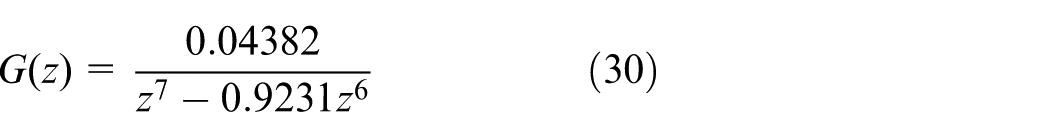
Meanwhile, the discrete model of Equation (29) is obtained as follows

Results and analysis
In the following, simulation results are conducted based on the obtained process models. Here, FO-PIDDMC is compared with the DMC using the integer order model shown in Equation (30). The FO-PIDDMC is designed based on the Oustaloup approximated model shown in Equation (31). Finally, the two obtained control laws are both implemented on the Oustaloup approximated model obtained through the real fractional-order process. The set-point is selected as
Model/plant match case
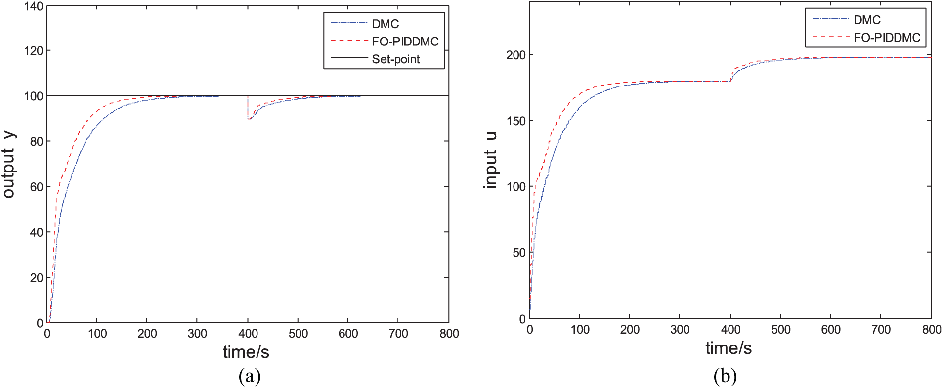
The parameters of the two controllers are set as
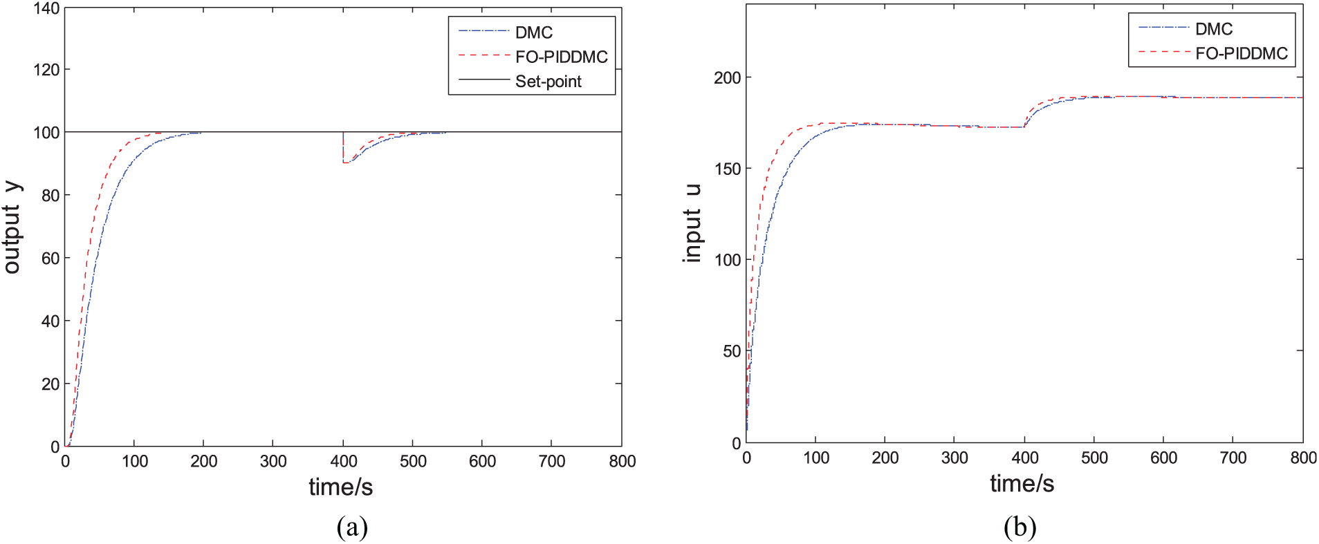
(a) Output responses under no model/plant mismatch and (b) input signals under no model/plant mismatch.
Model/plant mismatch case
Since there are often uncertain factors in practice causing a certain model/plant mismatch, this section will mimic such situation through Monte Carlo method. Here, three groups of random process parameters resulted from the ±
Case 1
Case 2
Case 3
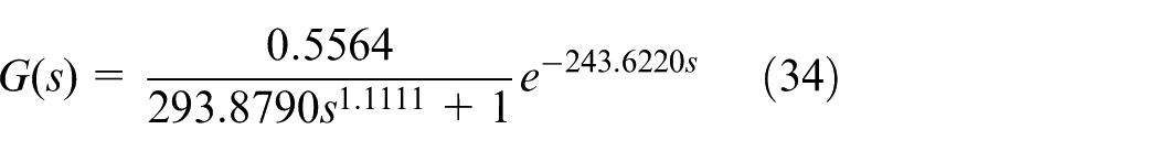
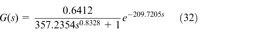
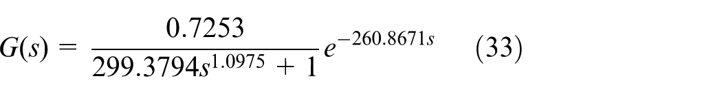
Now the controller of the FO-PIDDMC is still designed based on the nominal Oustaloup approximated model shown in Equation (31), and Equation (30) is still adopted as the model for the integer order DMC. However, the two obtained control laws are both implemented on the Oustaloup approximated models obtained through the real fractional-order processes shown in Equations (32)–(34).
The control parameters of the controllers remain unchanged as those in the model/plant match case. The results are shown in Figures 4–6. From the responses, it can be found that the control performance of the two models is still stable. However, we can easily find that the FO-PIDDMC yields improved control performance. Figure 4 shows that the response of the integer order DMC controller is relatively slower. The situations in Figures 5 and 6 are like those in Figure 4, where the FO-PIDDMC has faster response with better disturbance-rejection ability. In a word, FO-PIDDMC has improved dynamic response and robust performance.
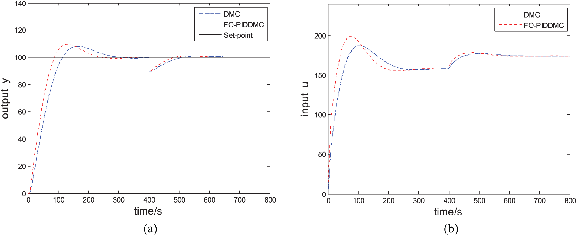
(a) Output responses for case 1 under model/plant mismatch and (b) input signals for case 1 under model/plant mismatch.
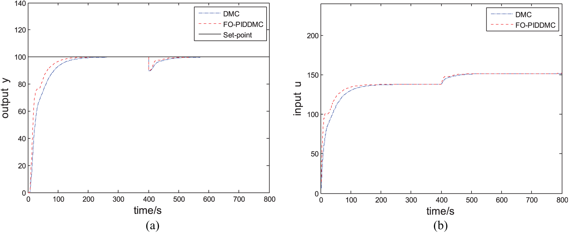
(a) Output responses for case 2 under model/plant mismatch and (b) input signals for case 2 under model/plant mismatch.
(a) Output responses for case 3 under model/plant mismatch and (b) input signals for case 3 under model/plant mismatch.
Conclusion
A PIDDMC using fractional-order modeling is presented. The proposed controller showed improved dynamic response and robust performance because the fractional-order modeling and flexible adjustment of control parameters are included in the controller design. Finally, the temperature control of a heating furnace verifies the effectiveness of the proposed method.
Footnotes
Declaration of conflicting interests
The author(s) declared no potential conflicts of interest with respect to the research, authorship, and/or publication of this article.
Funding
The author(s) received no financial support for the research, authorship, and/or publication of this article.