
Abstract
This paper presents a new hybrid metaheuristic model in order to estimate wind speeds accurately. The study was started by the training process of artificial neural networks with some metaheuristic algorithms such as evolutionary strategy, genetic algorithm, ant colony optimization, probability-based incremental learning, particle swarm optimization, and radial movement optimization in the literature. The success of each model is recorded in graphs. In order to make the closest estimation and to increase the system stability, a new hybrid metaheuristic model was developed using particle swarm optimization and radial movement optimization, and the training process of artificial neural networks was performed with this new model. The data were obtained by real-time measurements from a 63-m-high wind measurement station built at the coordinates of UTM E 263254 and N 4173479, altitude 1313 m. Two different scenarios were created using actual data and applied to all models. It was observed that the error values in the designed new hybrid metaheuristic model were lower than those of the other models.
Keywords
Introduction
Wind energy is an environment-friendly, unlimited, most economical type of energy which has a broad area of usage and is developing rapidly.1,2 However, the stochastic and intermittent structure of wind is the main factor that makes it difficult to estimate the speed and power of wind.3,4
The demand for electricity production by wind energy is accelerating day by day. This demand brings about an increase in the number of wind farms as well as some related problems. The main ones among these problems may be listed as grid reliability, power system quality, and interconnected linking operations.2,5,6 Performing procedures of wind speed and wind power estimation is effective in solving such problems. In addition, the procedure of wind speed and wind power estimation is also highly important in terms of determining the locations of new wind farms to be built, 7 facility maintenance and energy planning, 8 energy transformation efficiency and reduction of surge risks, 9 and optimal management of the benefits and risks of wind farms. 10 Wind speed and power estimation studies are discussed under four groups in terms of time. These are immediate-run estimation, short-run estimation, medium-run estimation, and long-run estimation.11–13
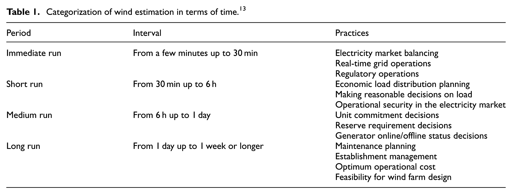
Wind speed and wind power estimation studies may also be categorized based on their estimation models as the persistence method,13–15 physical method, 16 statistical method, 17 and hybrid method. 18 The persistence method is the simplest method for estimating wind and is based on the assumption of a high correlation between the existent and future wind values. This method assumes that the wind speed value of any moment “t” will be the same as the value at a moment “t + Δt.”13,15 In the physical method, wind speed estimations are based on physical parameters and meteorological projections. The statistical method involves wind power estimations to be produced using past wind data.19,20 Table 1 shows the categorization of wind estimation in terms of time.
Categorization of wind estimation in terms of time. 13
While the physical method is highly successful in long-run estimations, the statistical method is successful in short-run estimations. The physical method uses parameters like terrain, slope, pressure, and temperature to make estimations of wind speed and power, while the statistical method uses statistical models.8,21,22 The hybrid method is a method that combines different methods that have unique abilities and characteristics. The purpose of such a method is to obtain the most suitable estimation performance by utilizing the advantages of each model that is included. 18 Studies in the literature developed hybrid models which utilized two, three, and even four components. Some of these studies are listed in Table 2.
Hybrid models for wind speed estimation in the literature.
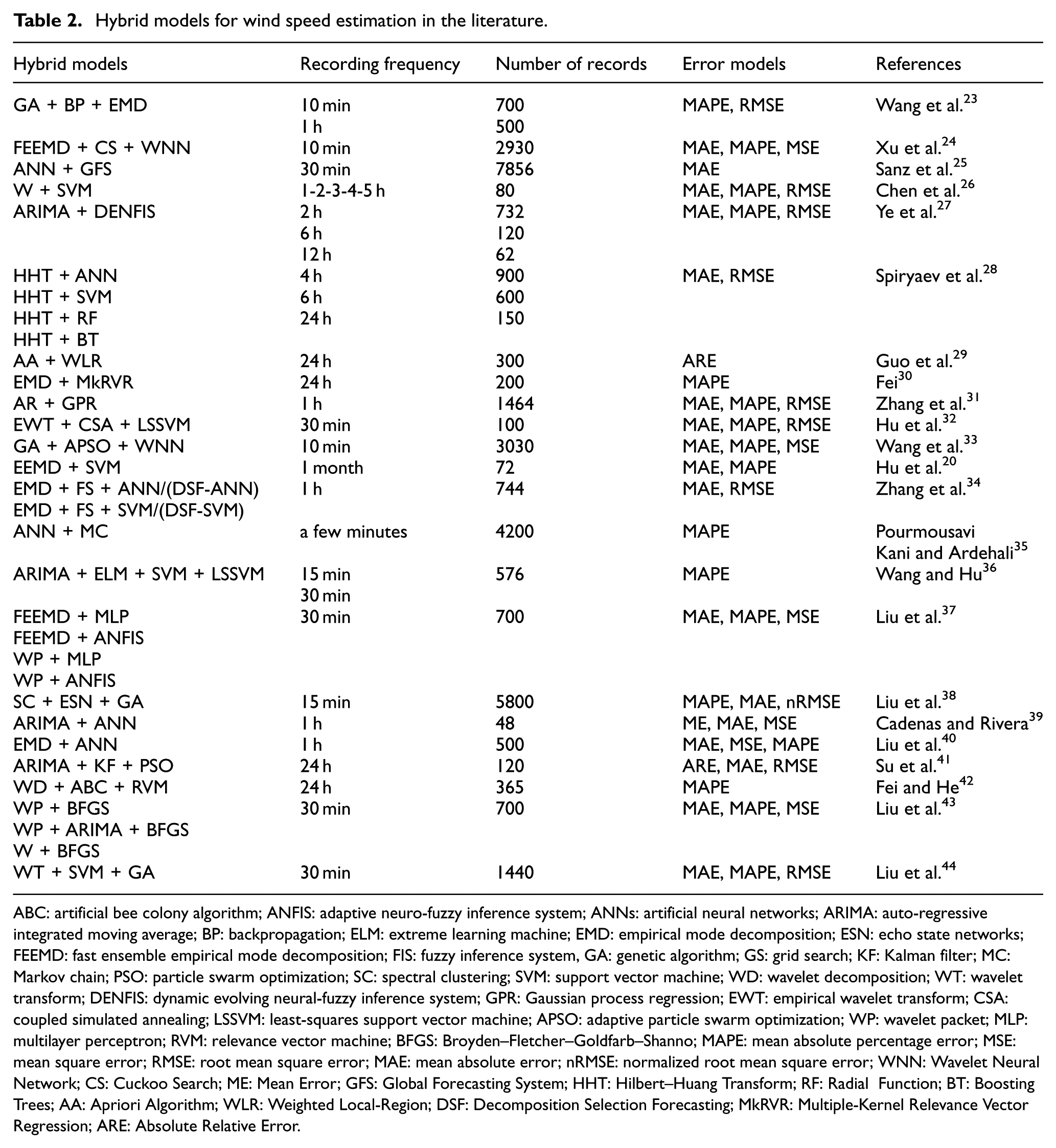
ABC: artificial bee colony algorithm; ANFIS: adaptive neuro-fuzzy inference system; ANNs: artificial neural networks; ARIMA: auto-regressive integrated moving average; BP: backpropagation; ELM: extreme learning machine; EMD: empirical mode decomposition; ESN: echo state networks; FEEMD: fast ensemble empirical mode decomposition; FIS: fuzzy inference system, GA: genetic algorithm; GS: grid search; KF: Kalman filter; MC: Markov chain; PSO: particle swarm optimization; SC: spectral clustering; SVM: support vector machine; WD: wavelet decomposition; WT: wavelet transform; DENFIS: dynamic evolving neural-fuzzy inference system; GPR: Gaussian process regression; EWT: empirical wavelet transform; CSA: coupled simulated annealing; LSSVM: least-squares support vector machine; APSO: adaptive particle swarm optimization; WP: wavelet packet; MLP: multilayer perceptron; RVM: relevance vector machine; BFGS: Broyden–Fletcher–Goldfarb–Shanno; MAPE: mean absolute percentage error; MSE: mean square error; RMSE: root mean square error; MAE: mean absolute error; nRMSE: normalized root mean square error; WNN: Wavelet Neural Network; CS: Cuckoo Search; ME: Mean Error; GFS: Global Forecasting System; HHT: Hilbert–Huang Transform; RF: Radial Function; BT: Boosting Trees; AA: Apriori Algorithm; WLR: Weighted Local-Region; DSF: Decomposition Selection Forecasting; MkRVR: Multiple-Kernel Relevance Vector Regression; ARE: Absolute Relative Error.
In this study, training studies of artificial neural networks (ANNs) were considered as a problem and it was aimed to develop a model to be used in the ANN training process which is accurate and fast and works stably. With this aim, the study was started using some metaheuristic algorithms in the literature in order to be used in the ANN training process. The success of the developed hybrid metaheuristic models of ANNs trained with evolutionary strategy (ES), ANNs trained with genetic algorithm (GA), ANNs trained with ant colony optimization (ACO), ANNs trained with probability-based incremental learning (PBIL), ANNs trained with particle swarm optimization (PSO), and ANNs trained with radial movement optimization (RMO) was recorded and plotted. In order to make the closest estimation and to increase the system stability, a new hybrid metaheuristic model was developed using PSO and RMO, and the training process of ANNs was performed with this new hybrid metaheuristic model. Two scenarios were created and all the models were applied. The data were used in scenarios obtained from a wind measurement station built in a 63-m-high university campus. The success of the new designed hybrid metaheuristic model (ANNs trained with PRO + RMO) was compared with that of the other hybrid models.
Data processing
As shown in Figure 1, the wind measurement station was mounted at the coordinates of UTM E 263254 and N 4173479 and an altitude of 1313 m by steel guy ropes.
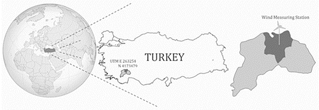
Geographical location of the wind measurement station.
The three-dimensional (3D) depiction of the wind measurement station is shown in Figure 2.
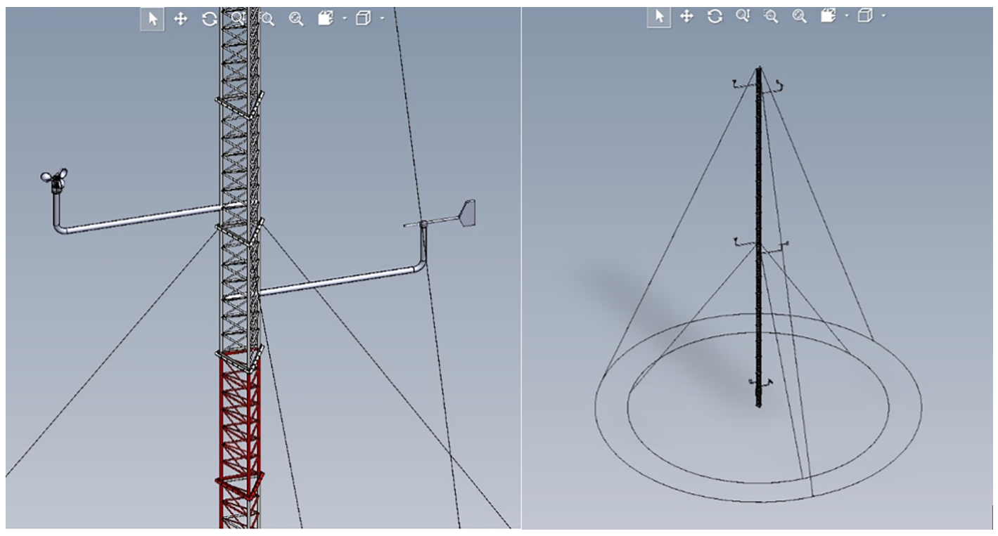
3D depiction of the wind measurement station.
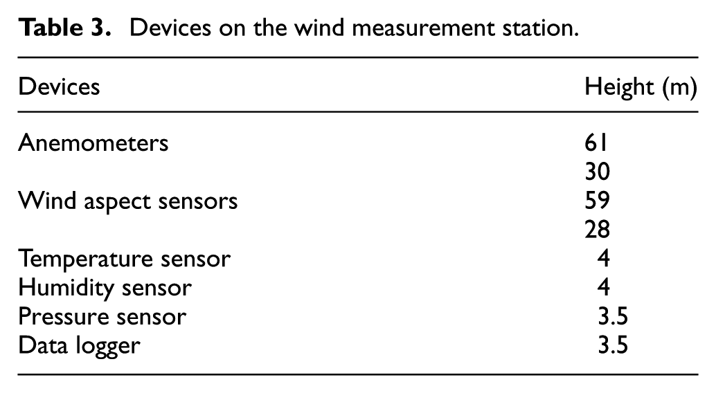
The measurement mast consisted of 21 modules of 3 m height and a total height of 63 m. The devices that were installed on the wind measurement station are given in Table 3.
Devices on the wind measurement station.
Installation works of the wind measurement station are shown in Figure 3.
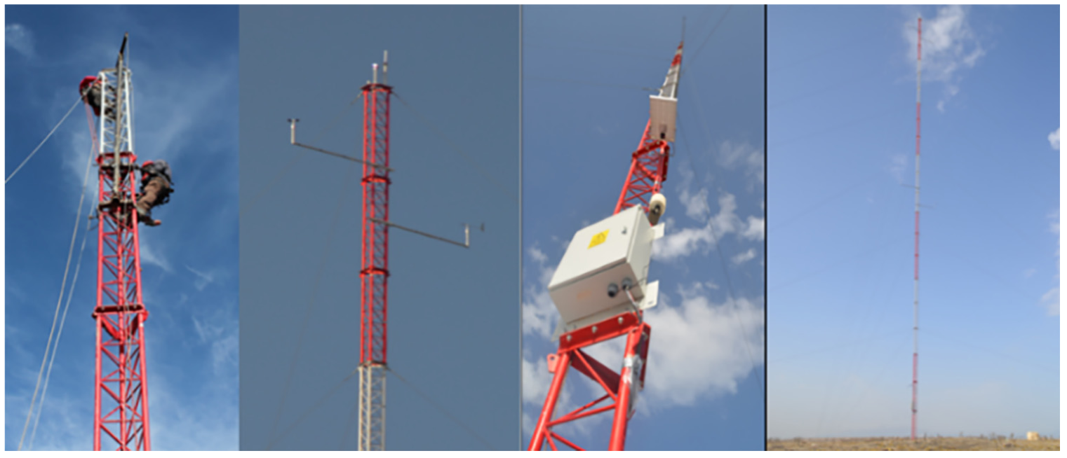
Installation works of the wind measurement station.
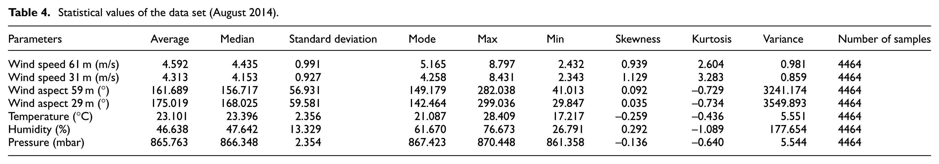
Statistical values of the data set (August 2014) are given in Table 4.
Statistical values of the data set (August 2014).
Design of a new hybrid metaheuristic model
Metaheuristic algorithms are one step higher than heuristic algorithms, and they can select and apply heuristic algorithms based on the solution of the problem. They have some advantages of minimizing the complexity of calculations, success in nonlinear problems, capabilities of recording previous findings in local searches, and possibilities of producing effective results within a short time.45–47 The algorithms that constituted the model are presented in sections “RMO” and “PSO.”
RMO
RMO is a swarm-based, fast, simple, and effective metaheuristic optimization model which uses the spherical boundaries of a vector in the search space to find the optimal solution and was designed for the spherical optimization of complex and nonlinear optimization problems. 46 In this algorithm, iteration cannot be transferred among the position and speed of the particles. Particles move from an updated point in each iteration, and therefore there is only a need for memory that has fewer calculations. The presence of a global best vector in the updating process prevents the algorithm from getting stuck in a local optimum. 48
The RMO algorithm is initiated by starting the particles in the search space that indicates the solutions of the problem. The positions of the particles are shown with a nop (number of particles) × nod (number of dimensions) matrix that is named as Xij. Nop is normally equal to the number of variables that would be optimized, but it can be selected by the user on demand.48,49
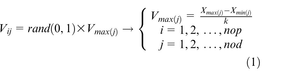
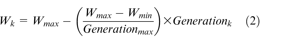
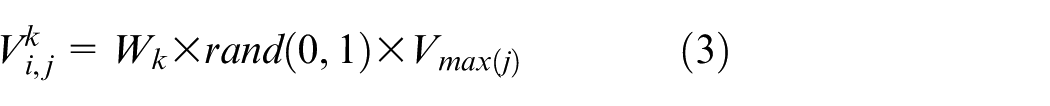
The step after obtaining the center point (cp) once is the dispersion of the particles from cp along the radius. This moves the particles from Vij-vector-based cp along the radius as straight lines. The Vij vector is a random nop × nop vector that is obtained by the equation below. The coefficient k in the equation should be a carefully selected integer45,47–49
As shown in equation (2), the speed vector has a weight of inertia (W) that is associated with and determines the convergence speed of the algorithm to an extent. This weight has a value that decreases along the generation iteration. Equation (2) shows the relationship between the weight of inertia and generation iterations45,47–49
As the speed vector
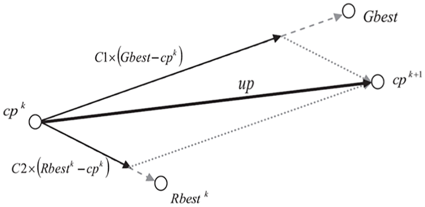
The particle that contains the optimal value is taken as the radial best (Rbest) vector. The accuracy value associated with the position of this particle represents the Rbest particle. The positions of the Gbest and Rbest particles are used along with the updating vector (up) to update the optimal center point position as shown in equations (4) and (5). C1 and C2 are the coefficients that need to be adjusted before running the algorithm47–49


Vectorial depiction of updating cp along the updating vector (up) is shown in Figure 4.
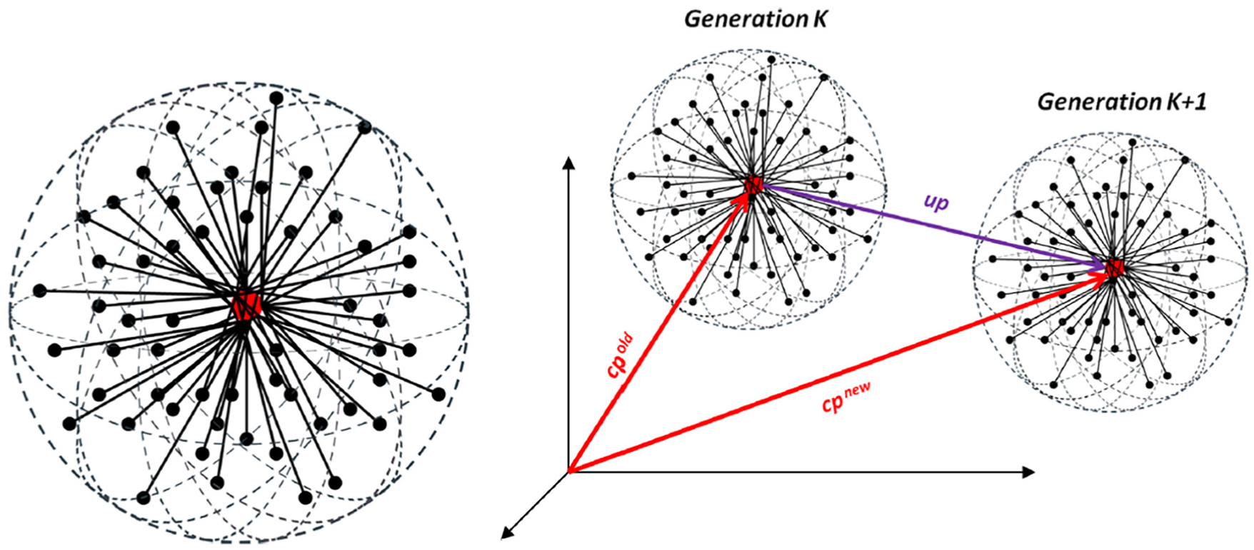
After the center point cp is updated, dispersion of the particles starts from the new cp. In the next generation, the Gbest value in the previous generation is updated by comparison to the Rbest value that is obtained during the dispersion of the particles in the new generation iteration. If Rbest provides a better solution than Gbest, their positions should be switched. The process continues until Gbest reaches a certain value or the number of generations reaches a defined maximum value.47,48 Figure 5 shows the sprinkling of the particles along the radii where Vmax is the radius of the sphere and updating the cp by up vector.
PSO
PSO is a two-dimensional simulation of the collective behaviors of swarms of birds and fish in cases such as looking for food. It is a metaheuristic algorithm. It is efficient and effective in terms of calculation and easy in terms of comprehension and implementation.50,51
PSO depicts each bird or fish as a particle and communities of birds or fish as swarms. In the algorithm, first, the initial positions, speeds, and population are randomly created. Accuracy values are calculated by determining the initial values for each particle in the population. The position value of the particle that has the best (minimum value) among the accuracy values is selected as Gbest. The other particles update their positions and speeds based on this value. The cycle continues until the finalization step. 52
In PSO,
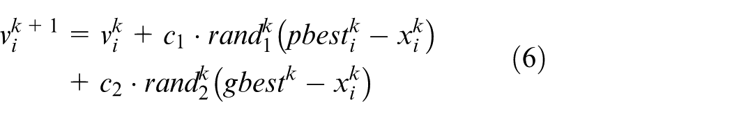

Figure 6 shows the vectorial depiction of the motion of a particle k.
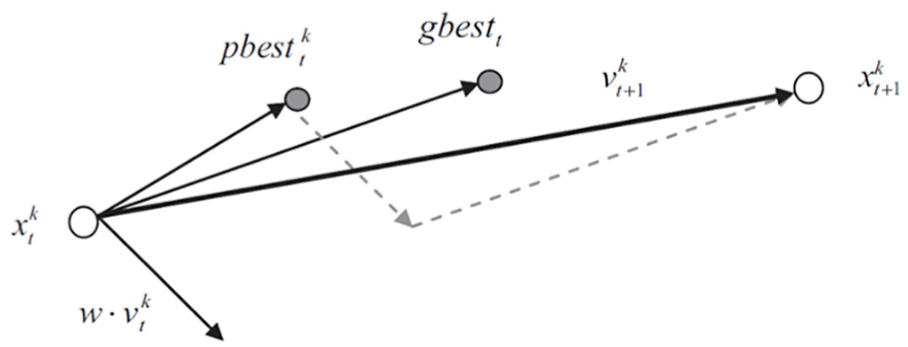
Vectorial depiction of the motion of a particle k. 7
A new hybrid metaheuristic model
The main aim here is to design a new hybrid metaheuristic model that is different to those in the literature, has high accuracy rates, is fast, and works stably. Thus, the model was developed using PSO and RMO, and the training process of ANNs was performed with this new model. With this training process, it is aimed to optimize the linear and nonlinear components of the data sets and large random fluctuations. The flowchart of the new model is shown in Figure 7.
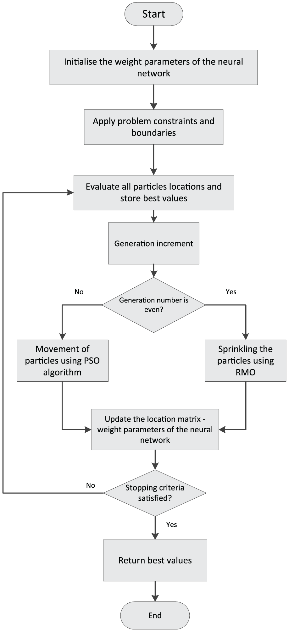
Flowchart of the new hybrid metaheuristic model.
This new hybrid metaheuristic model was designed to make these two different features in a hybrid algorithm by taking advantage of PSO and RMO’s distinctive individual features and to increase the system stability. Thus, PSO was used thanks to it’s features such as storage of coordinates and speeds of particles, ability to take into account the best available availability of particles, in determining the next movements, and it has benefited from its best past coordinates and its ability to consider the experiences of its most successful neighbor. Furthermore, RMO was used thanks to its excellent features such as the ability to search around the target point with an intensely focused feature, need for low memory, fast operation, and the ability to continue searching without getting pinched by the local optimum.
The data set was divided into three sets of data: 70% training, 15% verification, and 15% test data, while the model code is shown in Figure 8.

Dividing the data set into three parts.
Interface for new hybrid metaheuristic model (ANNs trained with PSO + RMO)
A user interface was designed using MATLAB App Designer software. Thus, a new and an alternative hybrid metaheuristic estimation model that is highly accurate, fast working, practical, and easy to use was supported by an interface. The characteristics of the designed interface are given below:
Allows selection of the file to be processed;
Displays information about the data set being processed;
Provides opportunity to use seven different estimation models (ANNs trained with ES, ANNs trained with GA, ANNs trained with ACO, ANNs trained with PBIL, ANNs trained with PSO, ANNs trained with RMO, and ANNs trained with PSO + RMO);
Allows drawing real-time plots of the actual and estimated values;
Can calculate six different error values such as normalized root mean square error (nRMSE), root mean square error (RMSE), mean square error (MSE), mean absolute percentage error (MAPE), peak signal-to-noise ratio (PSNR), and R and print them on the screen;
Allows easy modification of the Wmax, Wmin, c1, and c2 parameters for PSO + RMO, the W, C1, C2, and C3 parameters for RMO, and the Wmax, Wmin, c1, and c2 parameters for PSO;
Allows changing the number of iterations and number of particles (nop);
Allows plotting the Gbest values;
Can bring up real-time information about the stage of the process on the screen;
Can reset the command history with the “clear” button.
The interface designed using MATLAB App Designer is shown in Figure 9. The process starts by selecting the file to be run in the interface screen. Then the “create neural network” button is clicked on to create a neural network. The parameters in the bottom right corner of the screen are changed for a desired model (ANNs trained with ES, ANNs trained with GA, ANNs trained with ACO, ANNs trained with PBIL, ANNs trained with PSO, ANNs trained with RMO, ANNs trained with PSO + RMO) manually, that is, the parameter values that are considered to be the most suitable for a selected model are typed in. At this stage, it is also possible to change the number of iterations. Then the button for the desired model is clicked on. The progress of the process can be followed on the progress information part. After the process is completed, the actual and estimated values will be displayed on the screen along with the Gbest value. The error values (nRMSE, RMSE, MSE, MAPE, PSNR, R) are calculated one by one and shown on the error analysis part in the upper right corner of the screen.
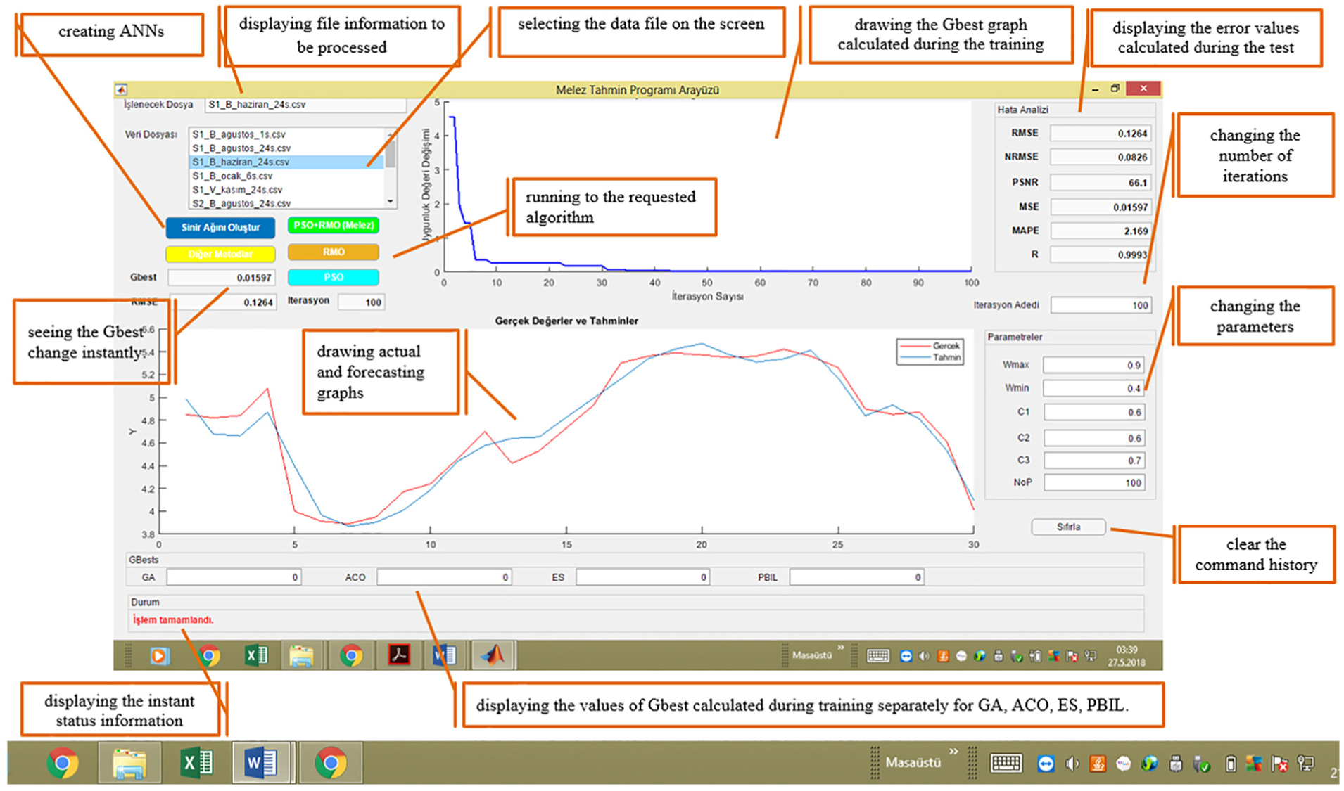
A user interface designed by MATLAB App Designer.
Furthermore, it was seen that the ES, GA, ACO, and PBIL metaheuristic algorithms have been applied in various fields to solve a large number of problems and the results have been presented.54–56 These metaheuristic algorithms were used in this paper, thanks to excellent contributions of the literature.
Performance results
This section examines the performance of the designed hybrid metaheuristic estimation model for wind speed estimations. For this aim, the data sets obtained from the wind measurement station were converted into two different scenarios, and the performance results of the hybrid metaheuristic estimation model are presented. Figure 10 which shows the scenario implementations:
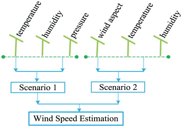
Scenario implementations.
Scenario 1. In this scenario, wind speed estimations were made according to the data on temperature, humidity, and pressure. The data used were recorded in January 2014 (recording frequency: 6 h, recording time: 10 days) and June 2014 (recording frequency: 24 h, recording time: 30 days).
Scenario 2. In this scenario, wind speed estimations were made according to the data on wind aspect, temperature, and humidity. The data used were recorded in August 2014 (recording frequency: 24 h, recording time: 15 days). The input and output variables used in Scenario 1 and Scenario 2 are shown in Table 5.
Input and output variables used in Scenario 1 and Scenario 2.
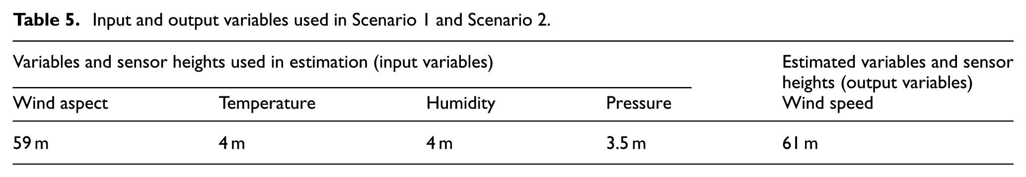
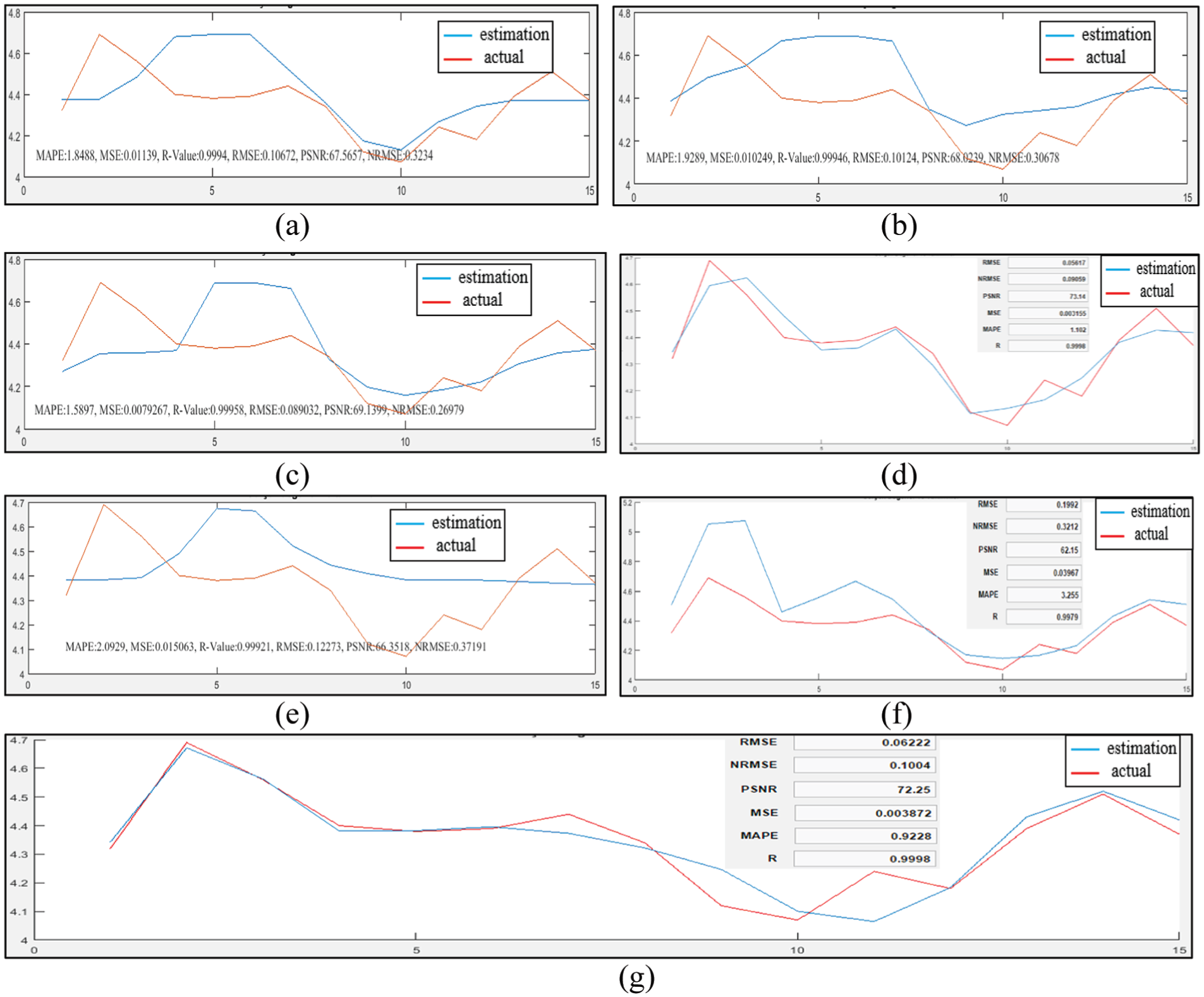
Figure 11 shows the actual and estimated plots of wind speed of Scenario 1—January. It includes the success of wind speed estimation of the hybrid models ANNs trained with ES, ANNs trained with PBIL, ANNs trained with GA, ANNs trained with PSO, ANNs trained with ACO, ANNs trained with RMO, and ANNs trained with PSO + RMO.
Actual and estimated plots of wind speed of Scenario 1—January: (a) ANNs trained with ES, (b) ANNs trained with PBIL, (c) ANNs trained with GA, (d) ANNs trained with PSO, (e) ANNs trained with ACO, (f) ANNs trained with RMO, and (g) ANNs trained with PSO + RMO (new hybrid metaheuristic model).
Figure 12 shows the actual and estimated plots of wind speed of Scenario 1—June. It includes the success of wind speed estimation of the hybrid models ANNs trained with ES, ANNs trained with PBIL, ANNs trained with GA, ANNs trained with PSO, ANNs trained with ACO, ANNs trained with RMO, and ANNs trained with PSO + RMO.
Actual and estimated plots of wind speed of Scenario 2—June: (a) ANNs trained with ES, (b) ANNs trained with PBIL, (c) ANNs trained with GA. (d) ANNs trained with PSO, (e) ANNs trained with ACO, (f) ANNs trained with RMO, and (g) ANNs trained with PSO + RMO (new hybrid metaheuristic model).
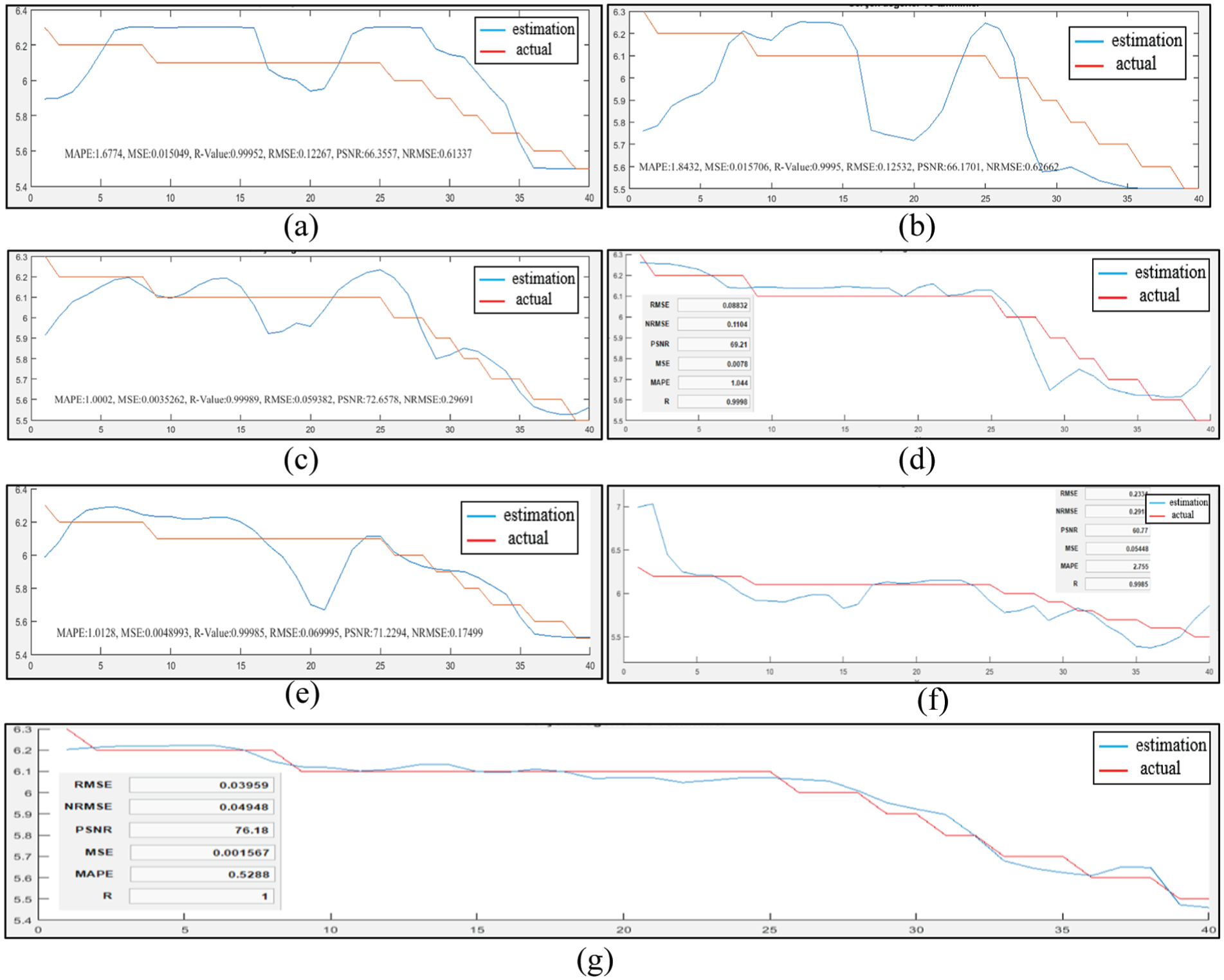
Figure 13 shows the actual and estimated plots of wind speed of Scenario 2—August. It includes the success of wind speed estimation of the hybrid models ANNs trained with ES, ANNs trained with PBIL, ANNs trained with GA, ANNs trained with PSO, ANNs trained with ACO, ANNs trained with RMO, and ANNs trained with PSO + RMO.
Actual and estimated plots of wind speed of Scenario 2—August: (a) ANNs trained with ES, (b) ANNs trained with PBIL, (c) ANNs trained with GA, (d) ANNs trained with PSO, (e) ANNs trained with ACO, (f) ANNs trained with RMO, and (g) ANNs trained with PSO + RMO (new hybrid metaheuristic model).
The best nRMSE, RMSE, MSE, MAPE, PSNR, and R values for the test error (50 runs) of Scenario 1—January are shown in Table 6. The min, average, max, and standard deviation values for Scenario 1—January test error (MAPE, 50 runs) are given in Table 7.
The best nRMSE, RMSE, MSE, MAPE, PSNR, and R values for the test error (50 runs) of Scenario 1—January.

nRMSE: normalized root mean square error; RMSE: root mean square error; MSE: mean square error; MAPE: mean absolute percentage error; PSNR: peak signal-to-noise ratio; ANN: artificial neural network; ACO: ant colony optimization; ES: evolutionary strategy; PBIL: probability-based incremental learning; GA: genetic algorithm; PSO: particle swarm optimization; RMO: radial movement optimization.
The min, average, max, and standard deviation (SD) values for Scenario 1—January test error (MAPE, 50 runs).
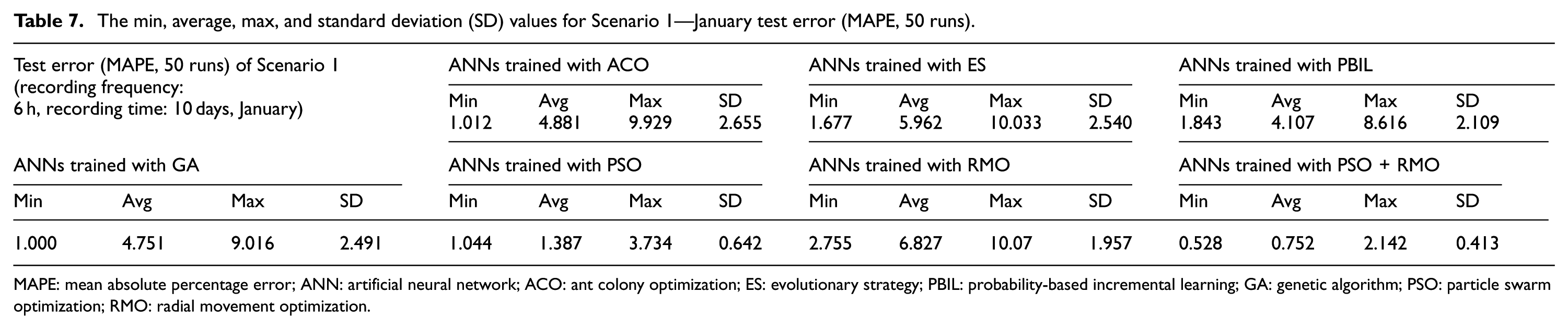
MAPE: mean absolute percentage error; ANN: artificial neural network; ACO: ant colony optimization; ES: evolutionary strategy; PBIL: probability-based incremental learning; GA: genetic algorithm; PSO: particle swarm optimization; RMO: radial movement optimization.
The best nRMSE, RMSE, MSE, MAPE, PSNR, and R values for the test error (50 runs) of Scenario 1—June are given in Table 8. The min, average, max, and standard deviation values for Scenario 1—June test error (MAPE, 50 runs) are given Table 9.
The best nRMSE, RMSE, MSE, MAPE, PSNR, and R values for the test error (50 runs) of Scenario 1—June.
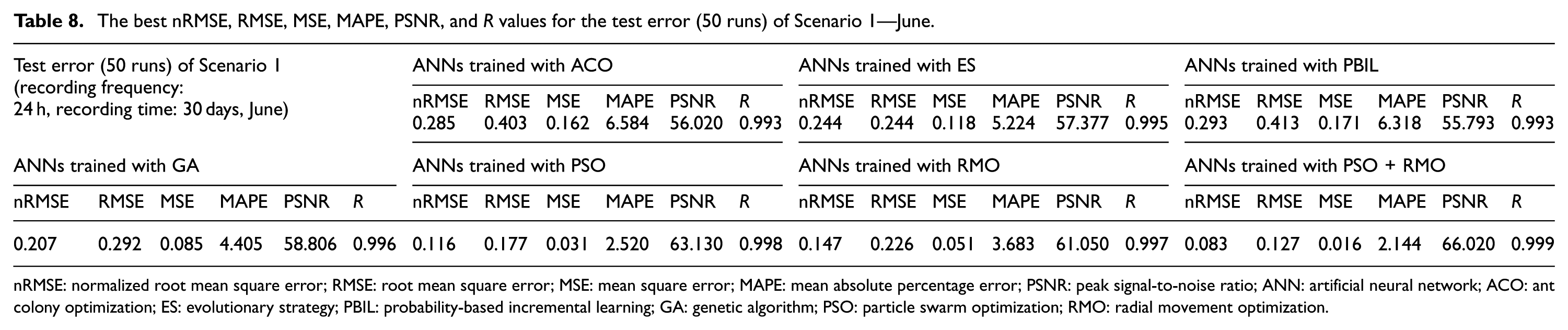
nRMSE: normalized root mean square error; RMSE: root mean square error; MSE: mean square error; MAPE: mean absolute percentage error; PSNR: peak signal-to-noise ratio; ANN: artificial neural network; ACO: ant colony optimization; ES: evolutionary strategy; PBIL: probability-based incremental learning; GA: genetic algorithm; PSO: particle swarm optimization; RMO: radial movement optimization.
The min, average, max, and standard deviation (SD) values for Scenario 1—June test error (MAPE, 50 runs).
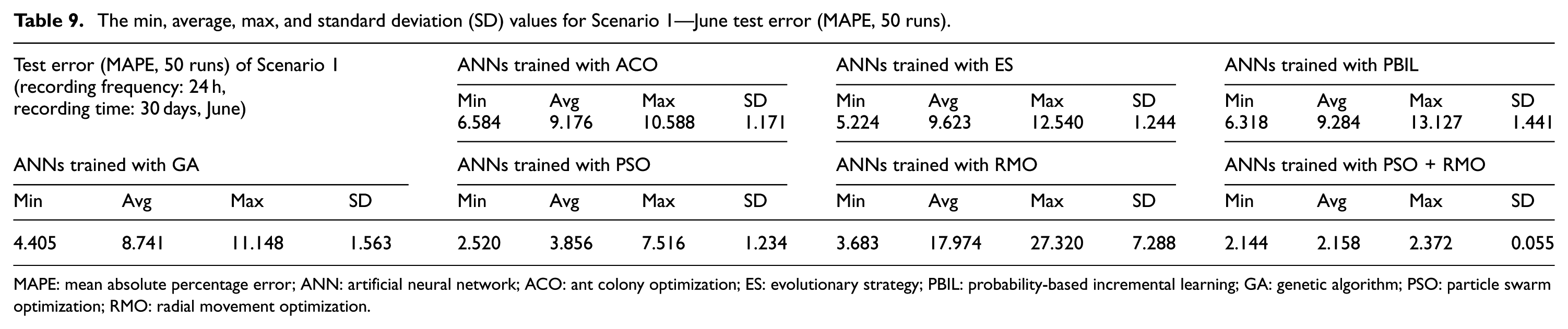
MAPE: mean absolute percentage error; ANN: artificial neural network; ACO: ant colony optimization; ES: evolutionary strategy; PBIL: probability-based incremental learning; GA: genetic algorithm; PSO: particle swarm optimization; RMO: radial movement optimization.
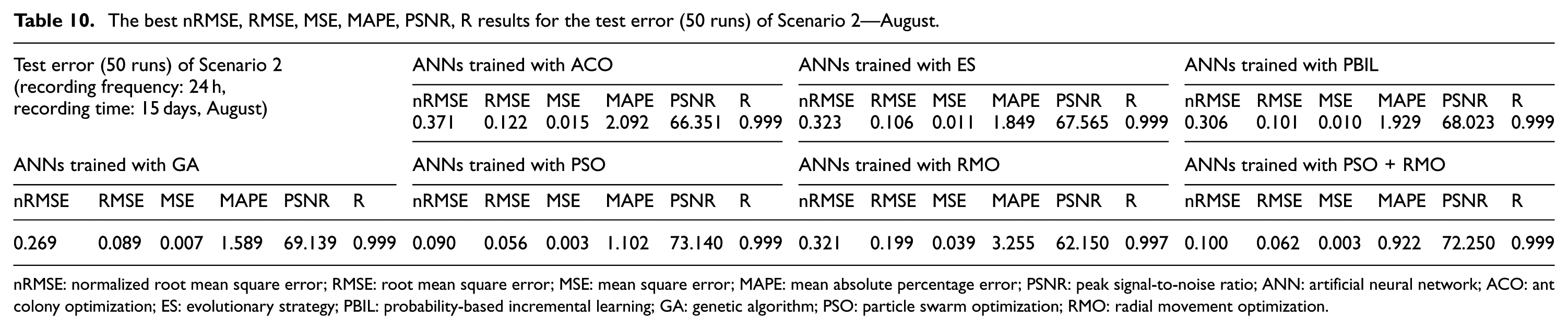
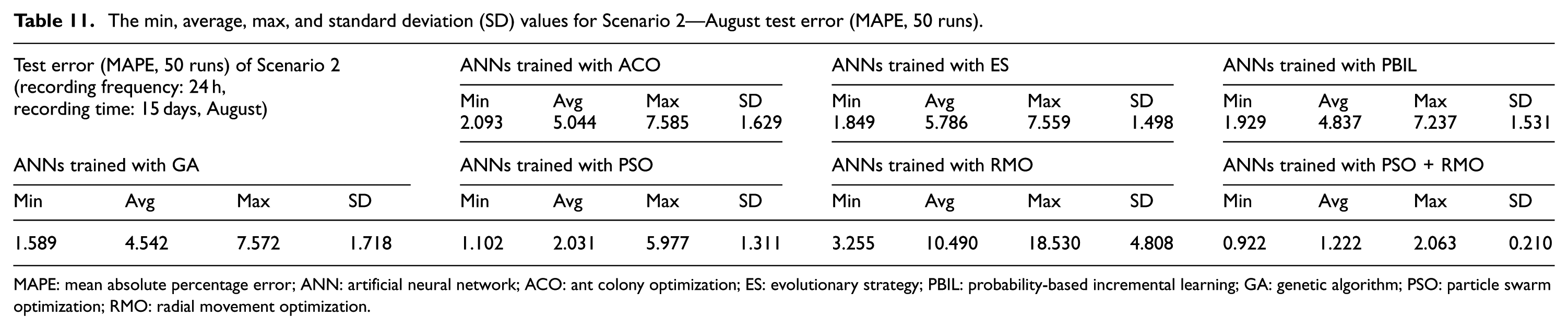
The best nRMSE, RMSE, MSE, MAPE, PSNR, and R values for the test error (50 runs) of Scenario 2—August are given in Table 10. The min, average, max, and standard deviation values for Scenario 2—August test error (MAPE, 50 runs) are given in Table 11.
The best nRMSE, RMSE, MSE, MAPE, PSNR, R results for the test error (50 runs) of Scenario 2—August.
nRMSE: normalized root mean square error; RMSE: root mean square error; MSE: mean square error; MAPE: mean absolute percentage error; PSNR: peak signal-to-noise ratio; ANN: artificial neural network; ACO: ant colony optimization; ES: evolutionary strategy; PBIL: probability-based incremental learning; GA: genetic algorithm; PSO: particle swarm optimization; RMO: radial movement optimization.
The min, average, max, and standard deviation (SD) values for Scenario 2—August test error (MAPE, 50 runs).
MAPE: mean absolute percentage error; ANN: artificial neural network; ACO: ant colony optimization; ES: evolutionary strategy; PBIL: probability-based incremental learning; GA: genetic algorithm; PSO: particle swarm optimization; RMO: radial movement optimization.
Conclusion
Wind may show momentary changes due to its nature, and it causes highly difficult and complicated estimations. Wind speed and wind power estimation studies done as accurately as possible are highly important in terms of determining the locations for wind farms, shaping energy unit costs, efficient and effective energy investments, and grid reliability.
In this study, a new hybrid metaheuristic (ANNs trained with PSO + RMO) estimation model was designed using the PSO and RMO models. It means that the training process of ANNs was performed using PSO and RMO. The designed new hybrid metaheuristic model was compared to each of the other hybrid models (ANNs trained with ES, ANNs trained with GA, ANNs trained with ACO, ANNs trained with PBIL, ANNs trained with PSO, and ANNs trained with RMO). An interface was designed using MATLAB App Designer (R2017b) and the whole model was visualized.
The performance of ANNs trained with ES, ANNs trained with GA, ANNs trained with ACO, ANNs trained with PBIL, ANNs trained with PSO, ANNs trained with RMO, and ANNs trained with the PSO + RMO combination were observed separately by two different scenarios (Scenario 1 and Scenario 2). According to the analysis of Scenario 1 (January and June) given in Tables 6 and 8, the nRMSE, RMSE, MSE, MAPE, PSNR, and R error values (test error, 50 runs) for the new hybrid metaheuristic model (ANNs trained with PSO + RMO) were much lower than those of the other hybrid models. Likewise, according to the analysis of Scenario 2 (August) given in Table 10, the nRMSE, RMSE, MSE, MAPE, PSNR, and R error values (test error, 50 runs) for the new hybrid metaheuristic model (ANNs trained with PSO + RMO) were much lower than those of the other hybrid models. It shows the success of the new designed hybrid metaheuristic estimation model.
The average MAPE values for Scenario 1 and Scenario 2 (test error, 50 runs) are shown in Figure 14. A newly designed hybrid metaheuristic model (ANNs trained with PSO + RMO) has achieved the most successful results among all the hybrid models. These are the lowest errors among the all models, 0.752, 1.222, and 2.158 for Scenario 1 (January), Scenario 2 (August), and Scenario 1 (June), respectively.
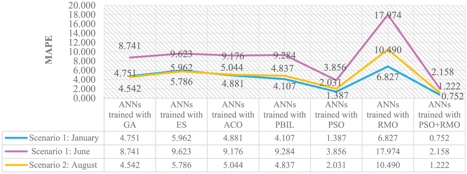
The average MAPE values for Scenario 1 and Scenario 2 (test error, 50 runs).
As a result of the analyses, it was observed that ANNs trained with the PSO + RMO model showed a highly accurate and reliable performance in the solution of nonlinear problems such as wind speed estimation. Thus, a new hybrid metaheuristic model (ANNs trained with PSO + RMO) which has high accuracy, is fast, and works stably has become a contribution to the literature with this study.
Footnotes
Acknowledgements
The authors thank the project coordinator Prof. Dr Serdar Salman who provided insight and expertise that greatly assisted the research. Furthermore, special thanks to Drs Rasoul Rahmani and İsmail Kırbaş for their excellent contribution to this study.
Declaration of conflicting interests
The author(s) declared no potential conflicts of interest with respect to the research, authorship, and/or publication of this article.
Funding
This research was supported by West Mediterranean Development Agency (BAKA, Project No. TR61/13/DFD/036) and Mehmet Akif Ersoy University Scientific Research Projects Commission (Project No. 0212-Gudumlu-13).