Sage Journals: Discover world-class research

Abstract

This study aims to solve the problem involving the high false alarm rate experienced during the detection process when using the traditional multivariate statistical process monitoring method. In addition, the existing model cannot be updated according to the actual situation. This article proposes a novel adaptive neighborhood preserving embedding algorithm as well as an online fault-detection approach based on adaptive neighborhood preserving embedding. This approach combines the approximate linear dependence condition with neighborhood preserving embedding. According to the newly proposed update strategy, the algorithm can achieve an adaptive update model that realizes the online fault detection of processes. The effectiveness and feasibility of the proposed approach are verified by experiments of the Tennessee Eastman process. Theoretical analysis and application experiment of Tennessee Eastman process demonstrate that in this article proposed fault-detection method based on adaptive neighborhood preserving embedding can effectively reduce the false alarm rate and improve the fault-detection performance.

Keywords

Adaptive neighborhood preserving embedding online fault detection manifold learning model updating

Introduction

With the increasing scale and complexity industrial process, the fault detection of the entire process has become the focus of research in the field of process control. Because the use of analytical methods and knowledge-based methods make it difficult to model complex industrial processes directly, and sensors are widely used in the industrial process, a lot of industrial process data can be preserved.^1,2 As a result, data-driven methods have received widespread attention and rapid development.^1,3–7 Industrial processes possess multiple characteristics, and monitoring these process characteristics independently can lead to false judgments. Therefore, there is a need for multivariate statistical process monitoring (MSPM).^8,9

MSPM is widely used in chemical, power, machinery, and others industrial processes based on the interrelationships between multiple sets of measurement data.^10,11–13 Process monitoring and fault-detection methods that are based on multivariate statistical projection theory are widely used.¹⁴ In MSPM, key information pertaining to the data is mapped into the low-dimensional space by the data dimension reduction, and the original high-dimensional data feature information is obtained, after which comprehensive statistics are established for the low-dimensional data to realize online monitoring. At present, MSPM methods include principal component analysis (PCA),^15,16 canonical correlation analysis (CCA),^17,18 independent component analysis (ICA),^19,20 Fisher discriminant analysis (FDA),^21,22 and partial least squares (PLS).^23,24

These methods usually assume that process variables are linearly related and obey the Gaussian distribution. For these problems, many extended methods have been developed, including kernel PCA,²⁵ dynamic PCA,²⁶ modified ICA,²⁷ dynamic ICA,²⁸ kernel FDA,²⁹ kernel PLS,³⁰ and dynamic kernel PLS.³¹ Although the above-mentioned methods and extended methods are widely used in fault detection. These methods can only capture the global variability of the process data, the detailed local neighborhood structure on the data manifold, which is proved to be more successful in identifying that the underlying data structures are failed to be discovered. As a result, the dimensionality reduction performance will be greatly degenerated without this crucial information. The global-based method mainly gives a constraint for the far away data points, which can guarantee their corresponding data points still faraway in low-dimensional mapping space. As a result, the intrinsic data structure may be distorted and the data points may be heavily overlapped in the reduced space. Through this point, a desirable projection should be the one that it can represent the local detailed geometry structure while modeling the process data.

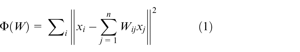
Recently, based on the limited understanding of the traditional global linear dimensionality reduction method, the manifold learning method has been developed. Locally linear embedding (LLE),³² locality preserving projections (LPP),³³ and neighborhood preserving embedding (NPE)³⁴ are the most widely used manifold learning methods. Most of the manifold learning methods use the local structure information of the data to reduce their dimension. NPE is a well-known manifold learning algorithm that is based on the idea of local data linearity and describes the local characteristics of the data to obtain the overall characteristics of the manifold structure. The algorithm is based on dimension reduction to extract the data characteristics, so low-dimensional spatial data can maximally retain reliable information about the original data. Hence, NPE can reveal the intrinsic geometrical structure of the observed data and find more meaningful low-dimensional information hidden in the high-dimensional observations compared with other methods. NPE has been used by engineers for process monitoring and fault detection. Song et al.³⁵ proposed a novel process monitoring in the Tennessee Eastman (TE) process via enhanced NPE. Yuan et al.³⁶ proposed a supervised NPE method for feature extraction and soft sensor modeling to improve the control of debutanizer column. Miao et al.³⁷ utilized the neighborhood preserving regression embedding (NPRE) method for nonlinear process soft sensor modeling to monitor fermentation process for penicillin production. In addition, Fan et al.³⁸ first proposed quality-relevant kernel NPE to detect abnormal and failure in the electro-fused magnesia furnace process.

However, the above NPE methods can only detect the process using the model that was initially established, and they cannot update the model according to the actual working condition, while the model lacks adaptability. Therefore, they will inevitably lead to high false alarm rates (FARs) in practice.³⁹ To solve the above problems, this article proposes an adaptive neighborhood preserving embedding (ANPE) algorithm method that can realize the online updating of the model and reduce FAR of the model. This proposed method combines traditional NPE and approximate linear dependence (ALD)^40,41 conditions. By calculating the approximate linear dependency between the new sample and the model, a new sample updating history model that satisfies the condition is selected to realize the adaptive updating of the model, and the online detection of the sampled data is achieved. At the same time, the adaptive update capability of the algorithm can ensure the continuous validity of the method. The proposed ANPE algorithm is verified by experiments of the TE process in this article.

The rest of this article is structured as follows. The concepts of NPE, ALD, and the inference procedure of the ANPE are introduced in section “Fault-detection method based on ANPE.” In section “Experiments using the TE process,” the performance of ANPE in fault detection is compared with that of NPE using the TE process.^42–45 Finally, conclusions are made in section “Conclusion.”

Fault-detection method based on ANPE

In this section, the related NPE algorithm and ALD condition were introduced and further described how to build ANPE algorithm and proposed online fault-detection method based on ANPE algorithm.

NPE algorithm

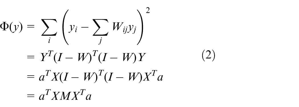
NPE is based on the idea of data local linearity, and its overall manifold structure characteristics are obtained by describing the local features of the data. More details about NPE can be found in He et al.³⁴

Suppose that the measurement matrix $X (x_{1}, \dots, x_{n}) \in R^{m}$ consists of n real-valued vectors. The ith column vector of X is $x_{i}$ . Based on the geometric intuitions that the global nonlinear data can be approximated with locally linear data, the local structure in NPE is characterized by coefficients that reconstruct each data point from its k-nearest neighbors. The reconstructed coefficient matrix W is obtained by minimizing the reconstruction error of Equation (1) by reconstructing the reconstruction coefficients of each sample using linear reconstruction^34,46

Φ (W) = \sum_{i} {‖ x_{i} - \sum_{j = 1}^{n} W_{ij} x_{j} ‖}^{2}

(1)

$W_{ij}$ represents the contribution of the data point $x_{j}$ to the reconstruction $x_{i}$ in the k neighborhoods of $x_{i}$ , $\sum_{j = 1}^{n} W_{ij} = 1$ . Each data point is reconstructed only by its nearest neighbor, and when $x_{j}$ is not a neighborhood of $x_{i}$ , $W_{ij} = 0$ . W in Equation (1) can be transformed into a least-squares problem with a constraint. The goal of the NPE algorithm is to find a set of projection vectors $a_{1}, a_{2}, \dots, a_{d}$ and the low-dimensional space $Y (y_{1}, \dots, y_{n}) \in R^{d} (d ⩽ m)$ after the projection has a local structure that is similar to the original space. Each data point can still be reconstructed by its corresponding neighbors at the same weight, and the projection matrix can be transformed into solving the problem of minimizing Equation (2)^34,46

\begin{matrix} Φ (y) = \sum_{i} {(y_{i} - \sum_{j} W_{ij} y_{j})}^{2} \\ = Y^{T} (I - W)^{T} (I - W) Y \\ = a^{T} X (I - W)^{T} (I - W) X^{T} a \\ = a^{T} XM X^{T} a \end{matrix}

(2)

In the formula, $M = (I - W)^{T} (I - W)$ . The constraint is $y^{T} y = a^{T} X X^{T} a^{T} = 1$ . It solves the problem of the minimum projection vector of the target function and transforms it into the generalized eigenvalue problem in Equation (3)

XM X^{T} a = λ X X^{T} a

(3)

Easy to get, $XM X^{T}$ and $X X^{T}$ are semi-definite matrices. In order to solve the generalized eigenvalue problem of the above equation, the eigenvectors corresponding to the smallest d eigenvalues $(λ_{1} ⩽ λ_{2}, \dots, ⩽ λ_{d})$ constitute the projection matrix $A = (a_{1}, a_{2}, \dots, a_{d})$ .

ALD

The ALD condition can check the linear dependency relationship between the new sample and the modeling sample, and it can effectively reduce the computational load caused by the sample update strategy. It is often used as the update decision condition of the model. More details about ALD can be obtained in Engel et al.⁴⁰ and Tang et al.⁴¹

When the historical model selects new samples for model updating, the diversity and independence of these samples should be considered. To ensure the applicability of the model, the independent new sample should be selected for model updating, so this article selects the ALD condition to determine whether the new sample is available for model updates. The ALD update conditions are as follows³⁹

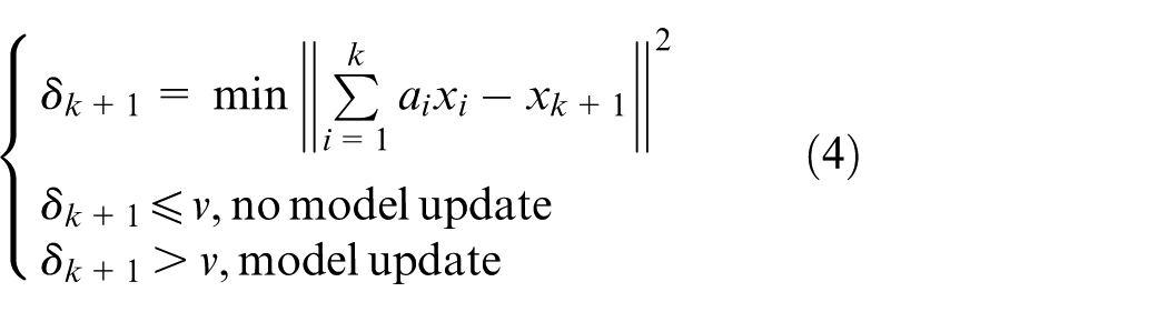
{\begin{matrix} δ_{k + 1} = min ‖ \sum_{i = 1}^{k} a_{i} x_{i} - x_{k + 1} ‖^{2} \\ δ_{k + 1} ⩽ v, no model update \\ δ_{k + 1} > v, model update \end{matrix}

(4)

In Equation (4), $x_{i} (i = 1, \dots, k)$ are the training samples, k is the number of samples, and $x_{k + 1}$ is the new sample. v is a pre-defined positive threshold, and $δ_{k + 1}$ is the approximate error value for the new sample. In addition, it determines whether or not to perform the model update based on the value of $δ_{k + 1}$ obtained by the ALD condition and the set threshold value v. If $δ_{k + 1} ⩽ v$ , no model update is performed; otherwise, it indicates that the new sample is relatively independent of the modeling sample and needs to be updated.

To solve Equation (4), Tang et al.⁴¹ give a concrete solution. When the new sample is added, by solving the differential of $δ_{k + 1}$ to a, the approximate error value $δ_{k + 1}$ of the new sample can be obtained. The relationship between the new sample and the model is as follows

δ_{k + 1} = k_{k + 1} - {\bar{k}}_{k}^{T} {\bar{K}}_{k}^{- 1} {\bar{k}}_{k}

(5)

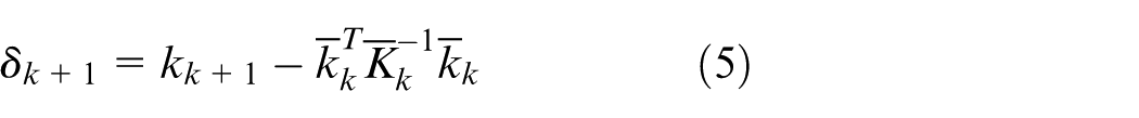
In Equation (5), $k_{k + 1} = x_{k + 1} \cdot x_{k + 1}^{T}$ is the normalized value of the new sample, $x_{k + 1}$ is the new sample normalized vector, ${\bar{K}}_{k} = X_{k} \cdot X_{k}^{T}$ is the modeling sample matrix, $X_{k}$ is the normalized vector for modeling the sample, and ${\bar{k}}_{k} = X_{k} \cdot x_{k + 1}^{T}$ is the modeling sample and the new sample correlation matrix.

When the update is determined according to the ALD condition, the selection of the threshold v is not systematic and can only be set by expert experience. While the higher threshold reduces the operating burden of the model, it reduces the accuracy of the model when detecting the fault. Furthermore, while the lower threshold can improve its accuracy, it also increases the computation and updates the time of the model. Therefore, it is very important to choose the right v.

ANPE Algorithm
1. Set threshold v; 2. Based on historical data to establish NPE off-line model $f_{0} (x)$ ; 3. For i = 1, 2, 3, … 4. Collect new sample $x_{i} (i = 1, \dots, k)$ ; 5. Obtain sample x_i online monitoring results according to existing model; 6. According to the results to determine whether the new sample x_i is fault data, when the statistic of new sample x_i is greater than its corresponding statistical limit, the sample is fault data, otherwise, it is normal data. 7. If x_i is not fault data; 8. Calculate ${\bar{k}}_{i - 1} (x_{i})$ ; 9. Calculate $δ_{i}$ according to Formula (5); 10. If $δ_{i} > v$ ; 11. Use the NPE algorithm to train the new sample $x_{i} (i = 1, \dots, k)$ to get the new model $F_{i} (x)$ ; 12. Update model $f_{i} (x) = F_{i} (x)$ , go back to step 3; 13. Else model $f_{i} (x)$ remains unchanged, go back to step 3 to re-detect the new sample; 14. End if 15. Else Model $f_{i} (x)$ remains unchanged. Go back to step 3 to re-detect the new sample; 16. End if 17. End for 18. Output the new model $f_{i} (x)$

ANPE Algorithm

1. Set threshold v;
2. Based on historical data to establish NPE off-line model

f_{0} (x)

;
3. For i = 1, 2, 3, …
4. Collect new sample

x_{i} (i = 1, \dots, k)

;
5. Obtain sample x_i online monitoring results according to existing model;
6. According to the results to determine whether the new sample x_i is fault data, when the statistic of new sample x_i is greater than its corresponding statistical limit, the sample is fault data, otherwise, it is normal data.
7. If x_i is not fault data;
8. Calculate

{\bar{k}}_{i - 1} (x_{i})

;
9. Calculate

δ_{i}

according to Formula (5);
10. If

δ_{i} > v

;
11. Use the NPE algorithm to train the new sample

x_{i} (i = 1, \dots, k)

to get the new model

F_{i} (x)

;
12. Update model

f_{i} (x) = F_{i} (x)

, go back to step 3;
13. Else model

f_{i} (x)

remains unchanged, go back to step 3 to re-detect the new sample;
14. End if
15. Else Model

f_{i} (x)

remains unchanged. Go back to step 3 to re-detect the new sample;
16. End if
17. End for
18. Output the new model

f_{i} (x)

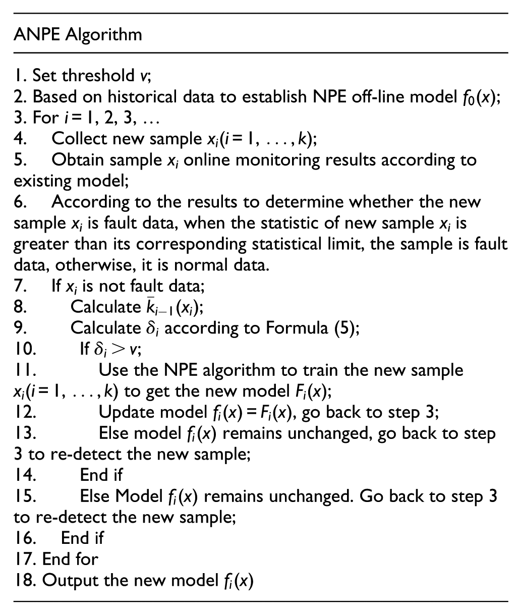
Description of ANPE algorithm

The ANPE algorithm comprises two parts: the offline modeling part based on NPE and the online part. The function of the offline modeling part is obtained by using the NPE algorithm based on the historical off-line data, and it is also the initial model.

The online part contains an online update module and an online fault-detection module. The online update module is used to assess the new sample according to the update strategy. If the new sample satisfies the strategy, then update the offline model with the valuable new sample to make the model adaptable to the actual situation. The role of the online fault-detection module is to monitor the new sample to determine whether a fault has occurred. Eventually, it achieves adaptive online fault detection.

The update strategy involves a comparison of online fault-detection results and ALD conditions. The detailed description of the updating strategy is to determine whether the new sample belongs to the faulty sample according to the online fault-detection module. If it is not a faulty sample, the ALD value of the sample is calculated according to Equation (5) for ALD conditions. When the calculated ALD value is greater than the set threshold v, it indicates that although the new sample is a normal sample, it fluctuates greatly with the training dataset, which meets the updating strategy. The new sample should be used as a training set to update the model.

When updating the model according to the fault-detection results and ALD condition, it is assumed that the point that needs to be updated is $x_{i} (i = 0, 1, \dots)$ , and the training length N remains unchanged each time that it is updated. That is, with the need to update the sample $x_{i}$ as the end, the N groups of continuous data, including $x_{i}$ , are used as the training sample, from $x_{i} + 1$ to $x_{i + 1}$ to detect the new sample, and the model is updated according to this class. The ANPE algorithm proposed in this article is summarized in the following using pseudocode.

Online fault-detection method based on ANPE

Based on the ANPE algorithm, an online fault-detection method based on ANPE is constructed. Then, the squared prediction error (SPE) statistic is introduced as the output of the model. The SPE is calculated as follows^47,48

SPE = ‖ \bar{x} ‖^{2} ⩽ δ^{2}

(6)

δ^{2} = g \cdot χ_{h}^{2}

(7)

g = var / 2 m

(8)

h = 2 m^{2} / var

(9)

In the above equations, $\bar{x}$ is the difference value between the original feature vector and the reconstructed feature vector, $δ^{2}$ is the control limit for SPE statistic, g is the weighting parameter included to account for the magnitude of SPE, $χ_{h}^{2}$ is a Chi-square distribution with h degree of freedom, and m and var are the mean and variance of the SPE statistic estimated from the training data, respectively.

The online fault-detection method based on ANPE uses the fault-detection rate (FDR) and FAR as performance indexes to measure the detection effect of the proposed method. The FDR and FAR are defined as follows⁹

FDR = \frac{N_{A}}{N_{TA}}

(10)

FAR = \frac{N_{N}}{N_{TN}}

(11)

In Equation (10), $N_{A}$ is the number that is judged as abnormal samples when the process is abnormal and $N_{TA}$ is the total number of the abnormal samples. In Equation (11), $N_{N}$ is the number that is judged as abnormal samples when the process is normal. $N_{TN}$ is the total number of the normal samples. The FAR is the proportion of data that exceeds the statistical control limits in normal data, and the FDR is the proportion of data that exceeds the statistical control limits in failure data. A larger value of the FDR indicates a better detection effect, while a lower FAR value implies an improved system performance.

Using Equations (7)–(9), when the training sample changes, the SPE statistic limit will change, and the corresponding FAR will change. Figure 1 shows the process of the online fault-detection method based on ANPE.

Figure 1.

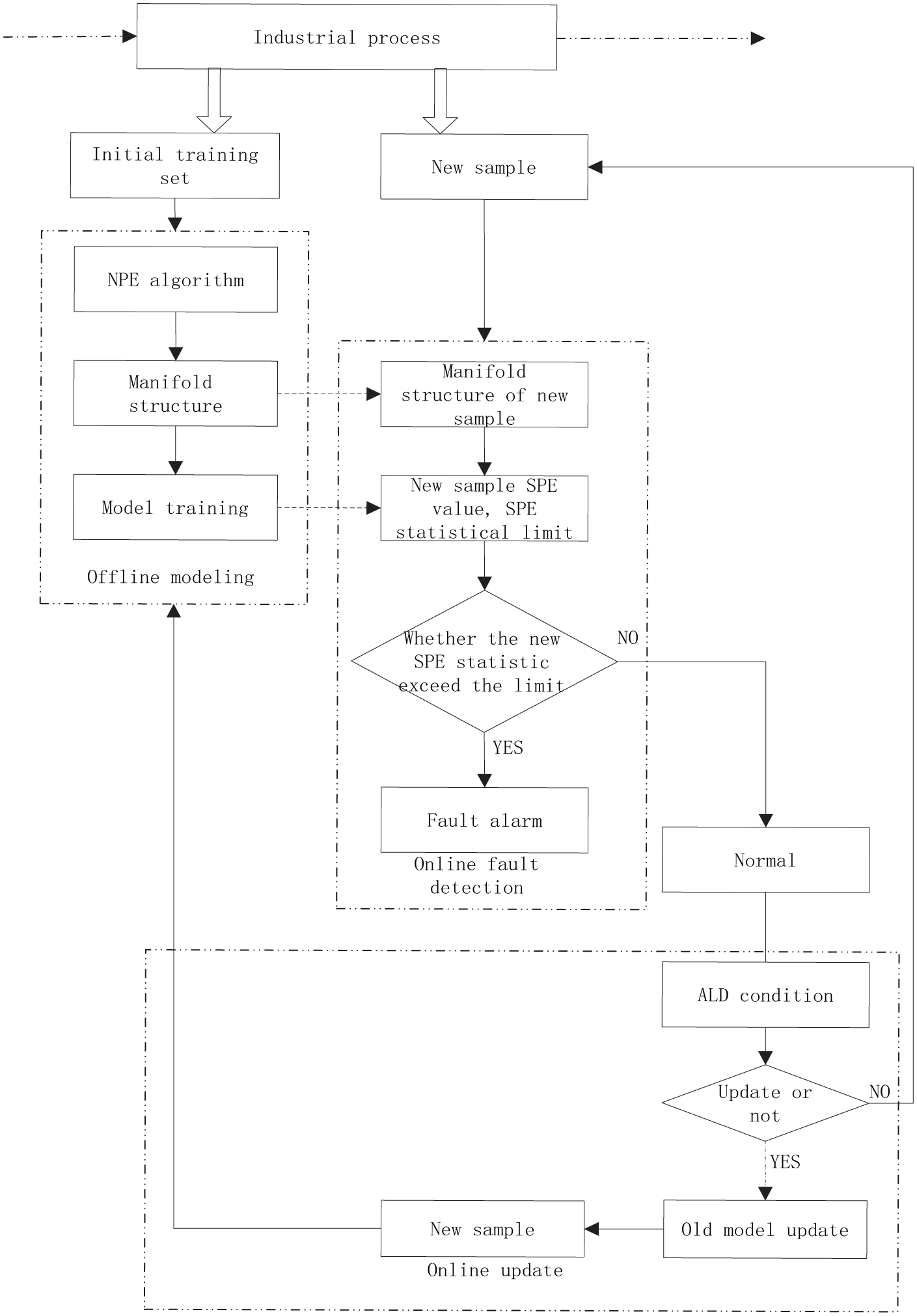
Flow chart of online fault-detection method based on ANPE.

From the flowchart, the working process of the proposed method can be determined as follows. First, the initial model is established by using the NPE algorithm according to the training dataset. Then, the SPE statistic of the new sample is calculated according to the stored old model, and it is then compared with the statistical limit.

Second, the SPE statistic of new samples is calculated and compared with the SPE statistical limit. If the SPE statistic is greater than the statistical limit, it indicates that a fault has occurred, and a fault-alarm signal is triggered; otherwise, it is the normal state.

Then, because the new sample is normal, the new sample’s ALD value needs to be calculated. If the ALD value is less than or equal to the set threshold v, no model update is performed; otherwise, the NPE model is re-trained and the old model is replaced. A new SPE statistical limit was obtained according to the output of NPE model based on new samples. Finally, the method realizes the online fault detection.

Experiments using the TE process

The performance of the proposed algorithm was verified using the TE process simulation. The ANPE algorithm was compared with the traditional NPE algorithm. The SPE statistic selects the control limit according to the 99% confidence level. In this experiment, k is the number of neighbors in the NPE algorithm, and d is the number of eigenvalues in the NPE algorithm. By dividing the neighborhood of the data, the initial data are divided into relatively small unit datasets, and the expected values can better balance the relationship between the local geometric features of the data and their global geometric features. When the selection of k values is relatively small, the data will be divided into many small neighborhoods, so the local geometric features of the process data cannot be effectively depicted. When k is larger, although more spatial information can be excavated, it can guarantee the intersection of neighborhoods. However, it requires extensive computations, and some unrelated data points may be included in the same neighborhood, so the assumption condition of local linearity is not satisfied. As the linear reconstruction reflects the local geometric information of the manifolds, the number of nearest neighbors is set based on the minimized reconstruction error of Equation (1). Considering and comparing several experiments, the nearest-neighbor number k of ANPE and NPE is set as 12. The number of the selected components d for dimensionality reduction in ANPE and NPE are determined according to the cumulative percent variance (CPV) criterion. In these experiments, d is chosen as 5 as the percent of variance accounted for 90% by these five selected factors. In other words, it means that the five selected factors can explain 90% of the original process data.

TE process

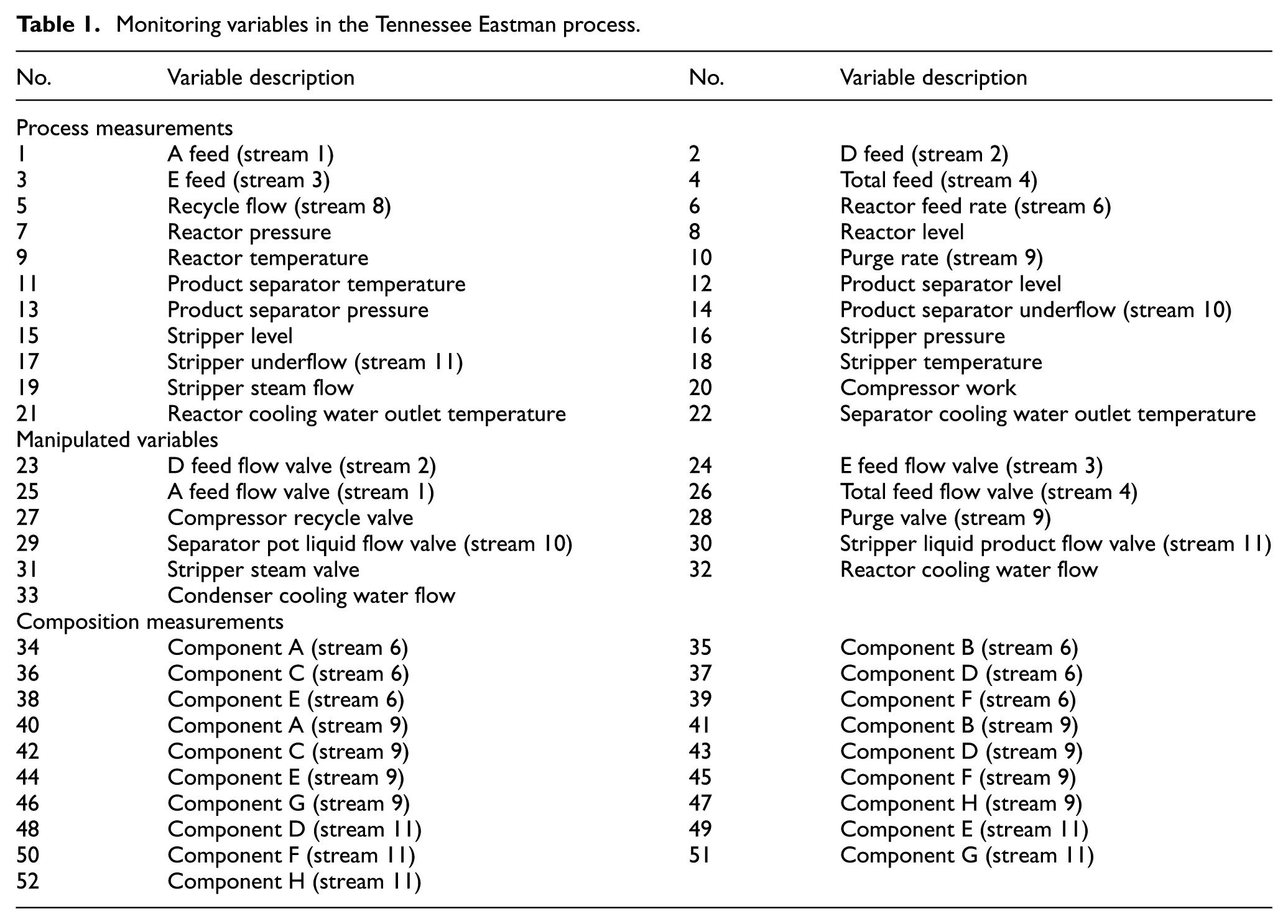
The TE process is a standard test platform that was developed by J. J. Downs and E. F. Vogel according to an actual chemical process developed by Eastman Chemical Company, which has become a common test platform for evaluating process control and fault-detection methods.^42–45,49 The TE model includes five major unit operations: a reactor, a condenser, a flash separator, a stripper, and a recycle compressor. There are four reactants A, C, D, and E; two products G and H; and one byproduct F. Figure 2 shows a flow chart of the TE process. As a simulation of a real industrial process, it contains 11 measurement variables, 22 continuous process measurements, and 19 manipulated variables. A total of m = 52 variables were recorded for all the manipulation and measurement variables, except for the agitation speed of the reactor’s stirrer. In this case study, all of the 52 variables were monitored. The complete list of variables is given in Table 1.^9,50 The TE process has one normal operating condition and 21 faulty operating conditions.⁵¹ The information about these faults is summarized in Table 2. The TE process sampling interval is 3 min, and a normal dataset and 21 fault datasets were acquired from the TE process.

Figure 2.

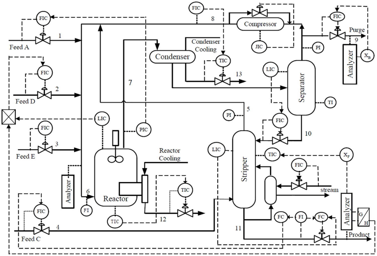
Flow chart of the Tennessee Eastman process.

Table 1.

Monitoring variables in the Tennessee Eastman process.

No.	Variable description	No.	Variable description
Process measurements
1	A feed (stream 1)	2	D feed (stream 2)
3	E feed (stream 3)	4	Total feed (stream 4)
5	Recycle flow (stream 8)	6	Reactor feed rate (stream 6)
7	Reactor pressure	8	Reactor level
9	Reactor temperature	10	Purge rate (stream 9)
11	Product separator temperature	12	Product separator level
13	Product separator pressure	14	Product separator underflow (stream 10)
15	Stripper level	16	Stripper pressure
17	Stripper underflow (stream 11)	18	Stripper temperature
19	Stripper steam flow	20	Compressor work
21	Reactor cooling water outlet temperature	22	Separator cooling water outlet temperature
Manipulated variables
23	D feed flow valve (stream 2)	24	E feed flow valve (stream 3)
25	A feed flow valve (stream 1)	26	Total feed flow valve (stream 4)
27	Compressor recycle valve	28	Purge valve (stream 9)
29	Separator pot liquid flow valve (stream 10)	30	Stripper liquid product flow valve (stream 11)
31	Stripper steam valve	32	Reactor cooling water flow
33	Condenser cooling water flow
Composition measurements
34	Component A (stream 6)	35	Component B (stream 6)
36	Component C (stream 6)	37	Component D (stream 6)
38	Component E (stream 6)	39	Component F (stream 6)
40	Component A (stream 9)	41	Component B (stream 9)
42	Component C (stream 9)	43	Component D (stream 9)
44	Component E (stream 9)	45	Component F (stream 9)
46	Component G (stream 9)	47	Component H (stream 9)
48	Component D (stream 11)	49	Component E (stream 11)
50	Component F (stream 11)	51	Component G (stream 11)
52	Component H (stream 11)

Table 2.

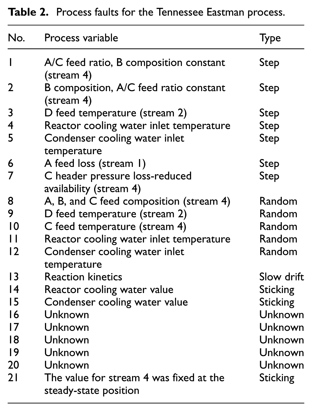
Process faults for the Tennessee Eastman process.

No.	Process variable	Type
1	A/C feed ratio, B composition constant (stream 4)	Step
2	B composition, A/C feed ratio constant (stream 4)	Step
3	D feed temperature (stream 2)	Step
4	Reactor cooling water inlet temperature	Step
5	Condenser cooling water inlet temperature	Step
6	A feed loss (stream 1)	Step
7	C header pressure loss-reduced availability (stream 4)	Step
8	A, B, and C feed composition (stream 4)	Random
9	D feed temperature (stream 2)	Random
10	C feed temperature (stream 4)	Random
11	Reactor cooling water inlet temperature	Random
12	Condenser cooling water inlet temperature	Random
13	Reaction kinetics	Slow drift
14	Reactor cooling water value	Sticking
15	Condenser cooling water value	Sticking
16	Unknown	Unknown
17	Unknown	Unknown
18	Unknown	Unknown
19	Unknown	Unknown
20	Unknown	Unknown
21	The value for stream 4 was fixed at the steady-state position	Sticking

Case study of the TE process

In this case study, a normal dataset has 960 samples. Each fault dataset consists of 960 samples, and all faults started at the 161st sample. This article compared the ANPE method with the NPE method proposed by He et al.³⁴ in 2005. The case study included the online monitoring of one normal operating condition and 21 faulty operating conditions.

During the monitoring of normal operating conditions, the duration of the training dataset sampling is 24 h, and the test dataset sampling period is 24 h. The number of training datasets is 480, and there are 480 test datasets. Experiments were performed using the ANPE method and the NPE method, and the FAR of the two methods was obtained under the normal situation according to Equations (10) and (11); the $N_{N}$ of NPE and ANPE methods in this experiments is 66 and 37, respectively. The monitoring results are shown in Table 3, and v is a pre-defined positive threshold in the ANPE method. However, for threshold v, there is still no scientific way to choose it, and it can only be set based on expert experience. While the higher threshold reduces the operating burden of the model, it reduces the accuracy with which the model detects the fault. Furthermore, the lower threshold can improve its accuracy and also increases the number of computations and updates the time of the model. After many experiments and comparisons, v was chosen as 29.3 in this case study for normal operating conditions. Figure 3 illustrates detailed monitoring results of two methods under normal situations: the blue curve is the SPE value of the model output and the red curve is the SPE statistical limit. It can be observed that the SPE statistical limit in Figure 3(a) is unvarying and it is varying in Figure 3(b), because the SPE statistical limit is online updated according to the ANPE method. So, the FAR in experiments using the ANPE method is less than using the NPE method. It is the same case in Figures 4 –8.

Table 3.

FAR of normal operating condition for the two methods.

Type	NPE	ANPE
Value	0.1375	0.0771

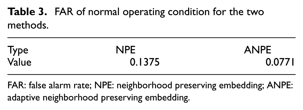
FAR: false alarm rate; NPE: neighborhood preserving embedding; ANPE: adaptive neighborhood preserving embedding.

Figure 3.

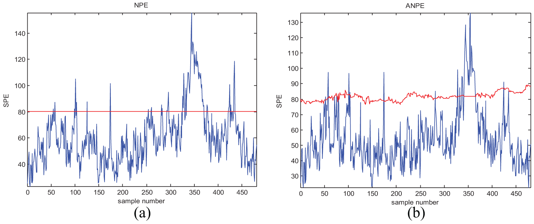
Monitoring results of normal operating condition with (a) NPE and (b) ANPE.

Figure 4.

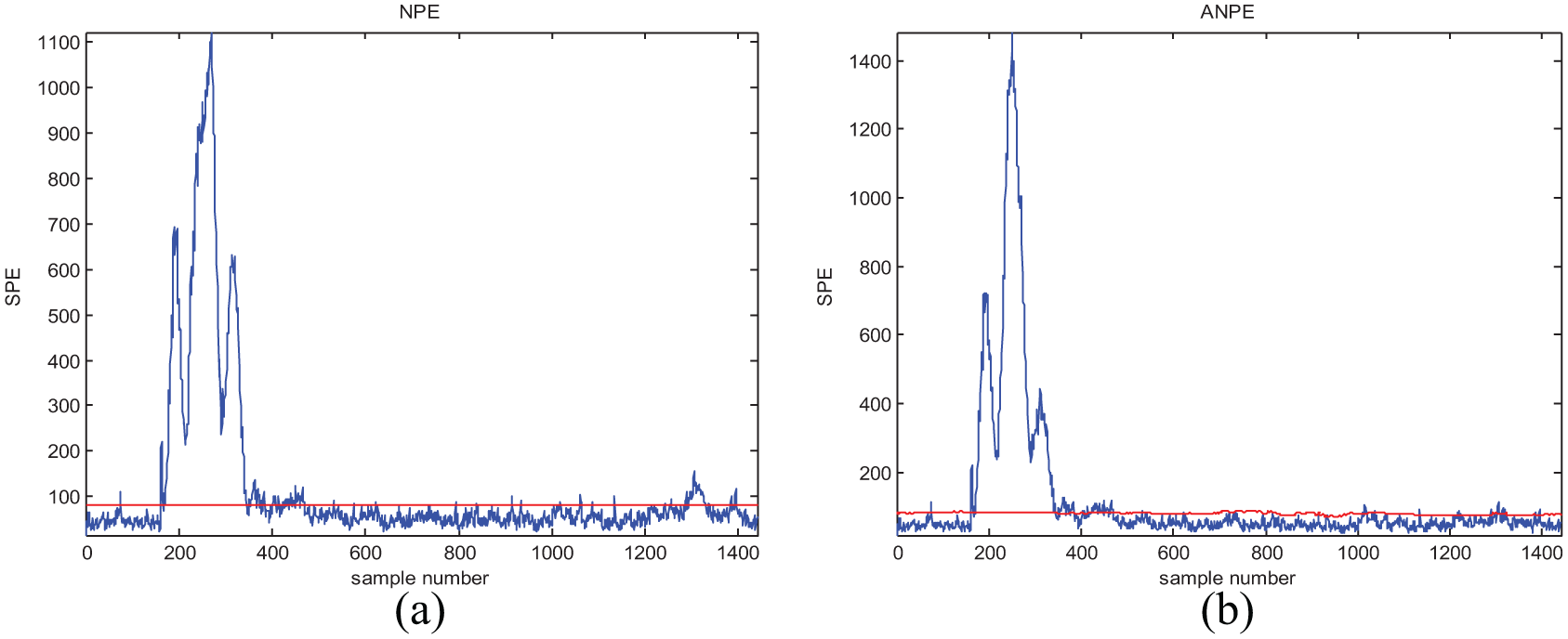
Monitoring results of fault 02 with (a) NPE and (b) ANPE.

Figure 5.

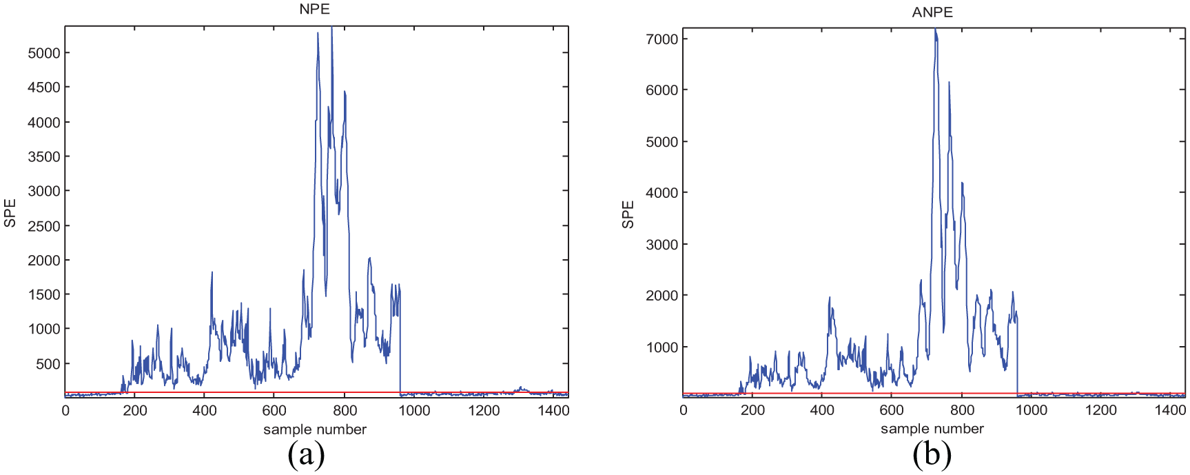
Monitoring results of fault 05 with (a) NPE and (b) ANPE.

Figure 6.

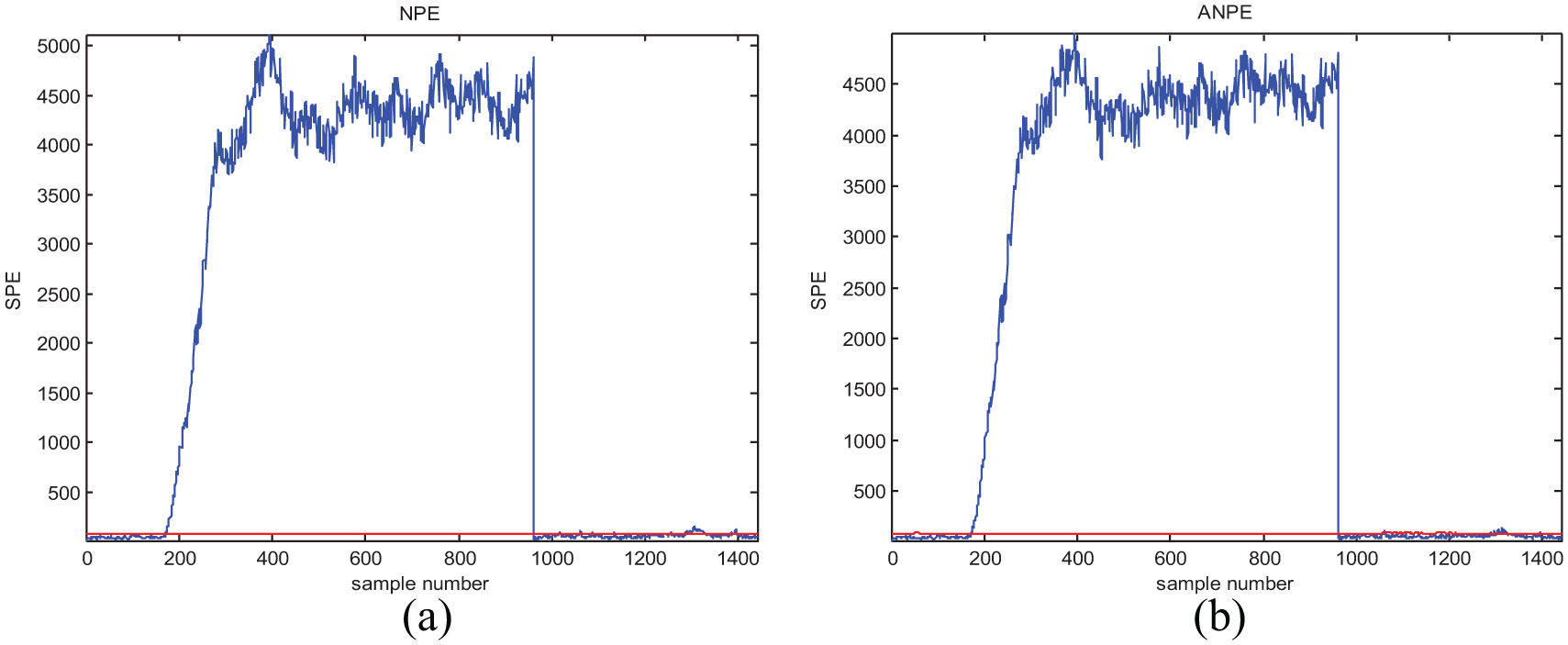
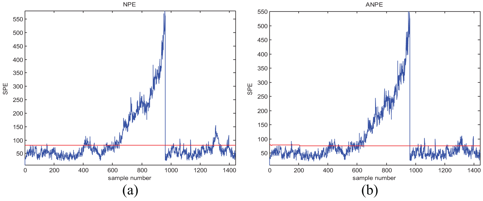
Monitoring results of fault 12 with (a) NPE and (b) ANPE.

Figure 7.

Monitoring results of fault 21 with (a) NPE and (b) ANPE.

Figure 8.

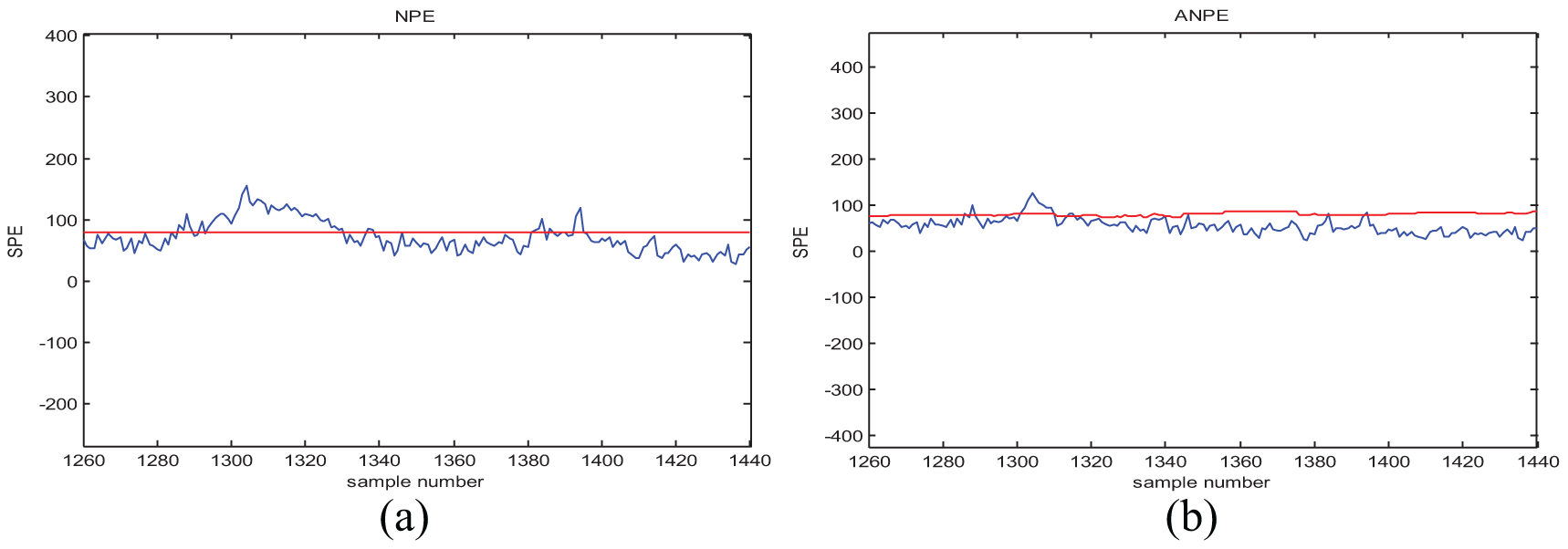
Enlarged view of 12 fault-monitoring results obtained with (a) NPE and (b) ANPE.

In the monitoring of 21 faulty operating conditions, the test dataset consisting of 960 faulty samples and 480 normal operation samples was collected. This article added a set of normal data after each fault dataset to simulate that the system works under normal operation conditions after the fault is repaired. Each training dataset is collected under normal operation conditions, and its sampling duration is 24 h and the number of training samples is 480. The test dataset was sampled for 72 h. The first 8 h is the normal data and the fault time is 40 h; the last 24 h is normal data and the number of test samples is 1440; all faults started at the 161st sample.

This article collected the FDR for the failure data and the FAR for the normal data. The monitoring results for the NPE and ANPE methods are presented in Table 4, and v is a pre-defined positive threshold in the ANPE method; the lower threshold can improve its accuracy, as well as increase the computation and update the time of the model. A larger FDR value indicates an improved detection effect; the lower the FAR value, the better the system performance. Figures 4 –8 show the detailed detection results of two methods for fault 02, 05, 12, and 21. Figure 8 gives an enlarged view of fault 12.

Table 4.

Monitoring results of faulty operating conditions for the two methods.

Fault	FDR of NPE	FDR of ANPE	FAR of NPE	FAR of ANPE	v
01	0.9950	0.9950	0.1047	0.0672	29.2
02	0.9862	0.9862	0.1047	0.0578	28.5
03	0.1263	0.1263	0.1063	0.0813	31.1
04	0.8938	0.8938	0.1063	0.1047	33.5
05	0.3362	0.3350	0.1063	0.0484	30.0
06	1.0000	1.0000	0.1031	0.0500	27.8
07	1.0000	1.0000	0.1031	0.0844	28.1
08	0.9800	0.9825	0.1141	0.0391	27.8
09	0.0925	0.0925	0.1641	0.1297	31.0
10	0.6188	0.6038	0.1063	0.0656	31.5
11	0.6737	0.6613	0.1047	0.0906	32.0
12	0.9888	0.9912	0.1078	0.0422	30.8
13	0.9475	0.9550	0.1078	0.0547	28.1
14	1.0000	1.0000	0.1047	0.0734	29.5
15	0.1638	0.1875	0.1031	0.0641	30.3
16	0.5250	0.5350	0.1812	0.1422	32.2
17	0.9013	0.8650	0.1047	0.0391	30.4
18	0.9013	0.9025	0.1047	0.0453	28.6
19	0.1400	0.1500	0.1031	0.0672	31.9
20	0.6225	0.5263	0.1031	0.0406	30.5
21	0.4888	0.4963	0.1047	0.0719	31.6

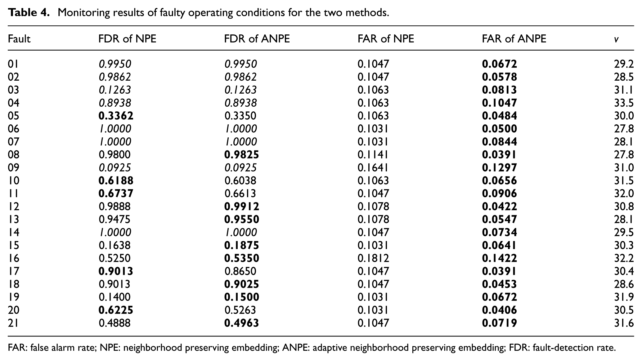
FAR: false alarm rate; NPE: neighborhood preserving embedding; ANPE: adaptive neighborhood preserving embedding; FDR: fault-detection rate.

In Figures 3 –8, the red line is the SPE statistical limit, and the blue line is the SPE statistic of the monitoring variables. Table 3 shows that the FAR of the ANPE method for the normal dataset is much lower than that of the NPE method, and the lower the FAR, the better the monitoring effect. Moreover, in Figure 3, because the ANPE method can be updated according to the online model, the SPE statistical limit has changed. According to Equations (7)–(9), you can find that when the training sample changes, the SPE statistic limit will change and the corresponding FAR will change. As the ANPE model was updated with new training samples, the number of samples ranges between 100–150, 200–300, and 400–450; the SPE statistical limit of the ANPE method is shifted upward, which reduces the FAR of the model. Based on the above results, this article further analyze the performance of the algorithm. The ANPE method provides a lower FAR than the NPE method, which verifies the effectiveness of the online monitoring method with adaptive capability.

From Table 4, we can see that for most kinds of process data, the ANPE method performs much better than NPE. In the monitoring of faults 01, 02, 03, 04, 06, 07, 09, and 14, ANPE and NPE obtain the same fault-detection results, but there are fewer false alarms for the ANPE method. In particular, ANPE achieves a better performance for most of the fault cases. During the monitoring process, ANPE not only has fewer false alarms but also performs better with respect to fault detection than NPE for faults 08, 12, 13, 15, 16, 18, 19, and 21. For the faults that are more difficult to detect, that is, faults 03, 09, and 15, both methods give a lower detection rate. This is because the duration of process data deviates from the normal fluctuation after a short fault occurs. In Figures 4(b), 5(b), 6(b), and 7(b), the ANPE method can detect the SPE statistics exceeding the limit, which indicates that the ANPE method can detect faults effectively. The fault-detection performance of the ANPE method depends on the fault type. When a fault occurs, the process data deviate from the normal fluctuations for long term; ANPE has a higher FDR, such as for fault 02 and fault 12. And if the process data deviate from the normal fluctuations for short term, the FDR of ANPE method will be low, like fault 03 and fault 21. However, the ANPE method can detect the occurrence of faults in time, even if the FDR for some fault types is relatively low. The enlarged view of fault 12 in Figure 8 shows that false alarms can be effectively reduced by updating the model online. Because the ANPE method can be updated according to the online model, the SPE statistical limit has changed. For cases where the number of samples ranges between 1280–1340 and 1380–1400, the SPE statistical limit of the ANPE method is shifted upward, which reduces the FAR of the model. According to the real-time data obtained to update the model online, the ANPE method will greatly improve the monitoring performance of the industrial process.

If considering the time delay of algorithm, the ANPE method may cost time more than about 1–2 s compared with the NPE method, and it is due to online updating the model according to ALD condition. In the TE process, the sampling period is 180 s, so a few seconds time delay dose not reduce the application effect of ANPE. But in some applications with high real-time requirement, the disadvantage of ANPE in time cost should be considered.

In summary, the case study verified that the proposed method can effectively reduce the FAR on the basis of guaranteeing the FDR and realizing the online accurate detection of industrial process faults. At the same time, the adaptive update capability of the algorithm ensures the real-time performance of the monitoring process and the continuous validity of the fault detection.

Conclusion

In order to reduce the FAR of fault detection for industrial processes, this article presents a new method based on the ANPE algorithm for fault detection, which is different from the traditional NPE method. The proposed method is based on offline training according to a set update strategy to determine whether the new sample can be used as a training sample to update the model. The model based on this method has the ability to perform adaptive updating and can achieve the online real-time monitoring of industrial processes. By performing simulation experiments involving the TE process, it is proven that the proposed method can reduce the FAR of the model while improving the effect of fault detection, and the effectiveness of the method in fault detection is explained. The method can be used for the online fault detection of industrial processes. In the future work, we plan to improve the algorithm proposed in this article using some optimization method to accommodate more process fault types, so that it can adaptively select thresholds v or others empirical parameters according to fault types and training sample. However, we also plan to present a new method to solve the online updating issue for time neighborhood preserving embedding (TNPE) algorithm.⁵²

Footnotes

Declaration of conflicting interests

The author(s) declared no potential conflicts of interest with respect to the research, authorship, and/or publication of this article.

Funding

This work was supported in part by the National Natural Science Foundation of China (NSFC; 61763049), the Science and Technology plan of Applied Basic Research Programs key Foundation of Yunnan province (2018FB112), the Science and Technology plan of Applied Basic Research Programs Foundation of Yunnan province (2017FB096), and the 8th Postgraduate Research and Innovation Project of Yunnan University.

Statement of data availability

Lei Tan and other co-authors allow readers to use any of the data in the manuscript.

ORCID iD

Peng Li

References

Qin

SJ.

Statistical process monitoring: basics and beyond. J Chemometric 2003; 17(8–9): 480–502.

Liu

Zhou

Lang

et al . Perspectives on data-driven operation monitoring and self-optimization of industrial processes. Acta Automat Sin 2018; 44(11): 1944–1956.

Frank

PM.

Fault diagnosis in dynamic systems using analytical and knowledge-based redundancy: a survey and some new results. Automatica 1990; 26(3): 459–474.

Patton

Chen

Review of parity space approaches to fault diagnosis for aerospace systems. Fault Detect Supervis Safe Tech Process 2012; 17(2): 65–81.

Wang

Ding

SX.

A new parity space approach for fault detection based on stationary wavelet transform. IEEE T Autom Control 2004; 49(2): 281–287.

Xiong

Wang

Niu

et al . A new multi-expert system applied in fault diagnosis. Electr Opt Control 2009; 16(7): 58–61.

Dokas

Karras

Panagiotakopoulos

DC.

Fault tree analysis and fuzzy expert systems: Early warning and emergency response of landfill operations. Environ Model Softw 2009; 24(1): 8–25.

Kano

Nakagawa

Data-based process monitoring, process control, and quality improvement: recent developments and applications in steel industry. Comput Chem Eng 2008; 32(1–2): 12–24.

A novel process monitoring and fault detection approach based on statistics locality preserving projections. J Process Control 2016; 37(5): 46–57.

10.

Xiao

YW.

Process monitoring based on wavelet transform principal component analysis and multiple support vector machines. Chin J Sci Instrum 2010; 31(3): 558–564.

11.

Shen

Song

ZQ.

Fault detection based on multivariate trajectory analysis. J Xi’an Jiaotong Univ 2017; 51(3): 122–128.

12.

Guo

Liu

Modeling and monitoring of multivariable wind turbine power curve. Power Syst Technol 2018; 42(10): 3347–3354.

13.

Kang

Han

Research on fault detection and diagnosis of refrigeration based on multivariate statistical analysis. Fluid Mach 2011; 39(6): 68–73.

14.

Tang

Liu

et al . New fault recognition method based on multivariate statistical process control. J Zhejiang Univ 2005; 39(5): 663–667.

15.

Storer

Georgakis

Disturbance detection and isolation by dynamic principal component analysis. Chemometric Intell Lab Syst 1995; 30(1): 179–196.

16.

Hirobayashi

Tamura

Yamamoto

Investigation of the surrounding environment’s influence on gait sensing using a plant as a sensor. J Sens 2009; 2009: 12.

17.

Russel

Chiang

Braatz

RD.

Fault detection in industrial processes using canonical variate analysis and dynamic principal component analysis. Chemometric Intell Lab Syst 2000; 51(1): 81–93.

18.

Lin

Bayesian information criterion based feature filtering for the fusion of multiple features in high-spatial-resolution satellite scene classification. J Sens 2015; 2015(1): 1–10.

19.

Lee

Qin

Lee

IB.

Fault detection and diagnosis based on modified independent component analysis. AICHE J 2006; 52(10): 3501–3514.

20.

Yang

Zhao

et al . Blind source separation model of earth-rock junctions in dike engineering based on distributed optical fiber sensing technology. J Sens 2015; 2015: 1–6.

21.

Qin

Wang

A new fault diagnosis method using fault directions in Fisher discriminant analysis. AICHE J 2005; 51(2): 555–571.

22.

Chiang

Kotanchek

Kordon

AK.

Fault diagnosis based on Fisher discriminant analysis and support vector machines. Comput Chem Eng 2004; 28(8): 1389–1401.

23.

Geladi

Kowalski

BR.

Partial least-squares regression: a tutorial. Analyt Chimica Acta 1986; 185(86): 1–17.

24.

Russell

Chiang

Braatz

RD.

Partial least squares. Adv Ind Control 2004; 69(4): 559–585.

25.

Liu

Yang

et al . Soft sensor of vehicle state estimation based on the kernel principal component and improved neural network. J Sens 2016; 2016(2): 1–8.

26.

Huang

Yan

Dynamic process fault detection and diagnosis based on dynamic principal component analysis, dynamic independent component analysis and Bayesian inference. Chemometric Intell Lab Syst 2015; 148: 115–127.

27.

Tong

Lan

Shi

Ensemble modified independent component analysis for enhanced non-Gaussian process monitoring. Control Eng Pract 2017; 58: 34–41.

28.

Stefatos

Hamza

AB.

Dynamic independent component analysis approach for fault detection and diagnosis. Expert Syst Appl 2010; 37(12): 8606–8617.

29.

Zhong

Zhang

Semisupervised kernel learning for FDA model and its application for fault classification in industrial processes. IEEE T Ind Inform 2016; 12(4): 1403–1411.

30.

Cao

Liang

et al . Exploring nonlinear relationships in chemical data using kernel-based methods. Chemometric Intell Lab Syst 2011; 107(1): 106–115.

31.

Jia

Zhang

Quality-related fault detection approach based on dynamic kernel partial least squares. Chem Eng Res Design 2016; 106: 242–252.

32.

Fang

et al . Dimensionality reduction of hyperspectral images based on robust spatial information using locally linear embedding. IEEE Geosci Remote Sens Lett 2017; 11(10): 1712–1716.

33.

Wang

et al . Robust locality preserving projections with cosine-based dissimilarity for linear dimensionality reduction. IEEE Access 2017; 5(99): 2676–2684.

34.

Cai

Yan

et al . Neighborhood preserving embedding. IEEE Int Conf Comput Vis 2005; 2(23): 1208–1213.

35.

Song

Tan

Shi

Process monitoring via enhanced neighborhood preserving embedding. Control Eng Pract 2016; 50: 48–56.

36.

Yuan

et al . Supervised neighborhood preserving embedding for feature extraction and its application for soft sensor modeling. J Chemometric 2016; 30(8): 430–441.

37.

Miao

LJ.

Neighborhood preserving regression embedding based data regression and its applications on soft sensor modeling. Chemometric Intell Lab Syst 2015; 147: 86–94.

38.

Fan

Zhang

et al . Fault detection for multimodal process using quality-relevant kernel neighborhood preserving embedding. Math Probl Eng 2015; 2015(6): 1–15.

39.

Bang

Yoo

Lee

IB.

Nonlinear PLS modeling with fuzzy inference system. Chemometric Intell Lab Syst 2002; 64(2): 137–155.

40.

Engel

Mannor

Meir

The kernel recursive least squares algorithm. IEEE T Signal Pr 2004; 52(8): 2275–2285.

41.

Tang

Chai

TY.

On-line principal component analysis with application to process modeling. Neuro Comput 2012; 82(1): 167–178.

42.

Downs

Vogel

EF.

A plant-wide industrial process control problem. Comput Chem Eng 1993; 17: 245–255.

43.

Chiang

Russell

Braatz

RD.

Fault diagnosis in chemical processes using Fisher discriminant analysis, discriminant partial least squares, and principal component analysis. Chemometric Intell Lab Syst 2000; 50(2): 243–252.

44.

Gao

Hou

An improved SVM integrated GS-PCA fault diagnosis approach of Tennessee Eastman process. Neurocomputing 2016; 174: 906–911.

45.

Yin

Wang

Gao

Data-driven process monitoring based on modified orthogonal projections to latent structures. IEEE T Control Syst Technol 2016; 24(4): 1480–1487.

46.

Roweis

Saul

LK.

Nonlinear dimensionality reduction by locally linear embedding. Science 2000; 290(5500): 2323–2326.

47.

Edward

JJ.

Multivariate quality control. Commun Stat Theory Method 1985; 14(11): 2657–2688.

48.

Lee

Yoo

Sang

et al . Nonlinear process monitoring using kernel principal component analysis. Chem Eng Sci 2004; 59(1): 223–234.

49.

Senoussi

Chebel-Morello

Denai

et al . Feature selection for fault detection systems: application to the Tennessee Eastman process. Appl Intell 2015; 44(1): 111–122

50.

Miao

Locality preserving based data regression and its application for soft sensor modeling. Canadian J Chem Eng 2016; 94(10): 1977–1986.

51.

Lau

Ghosh

Hussain

et al . Fault diagnosis of Tennessee Eastman process with multi-scale PCA and ANFIS. Chemometric Intell Lab Syst 2013; 120(2): 1–14.

52.

Miao

Song

et al . Time neighborhood preserving embedding model and its application for fault detection. Ind Eng Chem Res 2013; 52(38): 13717–13729.

Online process monitoring and fault-detection approach based on adaptive neighborhood preserving embedding

Abstract

Keywords

Introduction

Fault-detection method based on ANPE

NPE algorithm

ALD

Description of ANPE algorithm

Online fault-detection method based on ANPE

Experiments using the TE process

TE process

Case study of the TE process

Conclusion

Footnotes

Declaration of conflicting interests

Funding

Statement of data availability

ORCID iD

References