Sage Journals: Discover world-class research

Abstract

Inline inspection tools that are used to scan the interior defects of gas and oil pipelines tend to suffer from measuring error due to their sizing accuracy. This error often causes an over- or under-estimation of the operating conditions of the pipeline, which might lead to a system failure. While parametric calibration models provide a simple method to reduce the measuring error, it is limited to datasets that follow the normal distribution only. Thus, in this paper, a non-parametric calibration model based on k-nearest neighbor interpolation was proposed to improve the measurements recorded by the scanning tools. Corrosion data collected using an ultrasonic scan device and the magnetic flux leakage intelligent pig are considered in the research. The k-nearest neighbor interpolation is studied based on the effect of using six kernel functions with two different positioning approaches on the interpolation behavior. The results have shown enhancement in the accuracy of the readings obtained from the intelligent pig from ±20% of the pipeline wall thickness to only ±8%. This enhancement in the sizing accuracy is meant to prevent a possible system failure for using the corroded part of the studied pipeline for an extra 4.6 years instead of replacing it.

Keywords

Inline inspection error reduction corrosion measurement enhancement sizing accuracy

Introduction

Pipelines fulfilled the daily demand for oil and gas to the markets efficiently since 1879 when the first oil pipeline was built in Pennsylvania. Nowadays, pipelines are considered the fastest, safest, and most economical means to transport oil and gas. There are more than 3.5 million kilometers of oil pipeline crossing 120 countries around the world through networks that sometimes exceed 2000 km in length.^1–3 A periodical integrity assessment of the operational pipelines should be applied constantly to prevent the consequences of any system failure. Through its service time, aging pipelines are subjected to various corrosion mechanisms. These mechanisms are considered to be the defying factors affecting the integrity of the transfer system that may lead to failure.⁴ Since corrosion deteriorates the pipeline walls both internally and externally, the early and accurate detection of the actual remaining wall thickness of the operational pipeline through thorough inspection could potentially save the production circle from any halts. Inline inspection (ILI) tools, also known as non-destructive testing (NDT), are widely used to scan the interior of oil and gas pipeline for corrosion.⁵ Smart/intelligent pigs equipped with magnetic flux leakage (MFL-IP) sensors and ultrasonic scan devices are the two main types of metal-loss inspection techniques.^6,7 Both technologies scan the remaining pipeline wall thickness to decide the remaining operating lifetime of a pipeline. Some of the intelligent pigs used these days are supported with both MFL and ultrasonic testing (UT) sensors to do the scanning using both the technologies at the same time.^8–10 Each individual technology suffers from a different sizing accuracy and bears different properties. MFL-IP is used much often for corrosion and internal pipeline defect inspection. However, it has a lower sizing accuracy compared with other high-resolution scan devices and gives corrosion readings as relative measurements. On the other hand, the UT tool has a higher sizing accuracy and has the ability to give an actual measure for the remaining wall thickness making it a more accurate tool. The accuracy of corrosion measurements scanned using ILI tools is affected directly by its sizing accuracy. Table 1 shows the differences in the sizing accuracy for both devices^11,12 (t stands for pipeline nominal wall thickness).

Table 1.

Sizing accuracy of MFL and UT tools.

	MFL-IP		UT
Resolution	Standard	High	Extra high	High	Extra high
Sizing accuracy	±20%t	±10%t	±5%t	±6%t	±3%t
Confidence level	80%	80%	80%	80%	80%

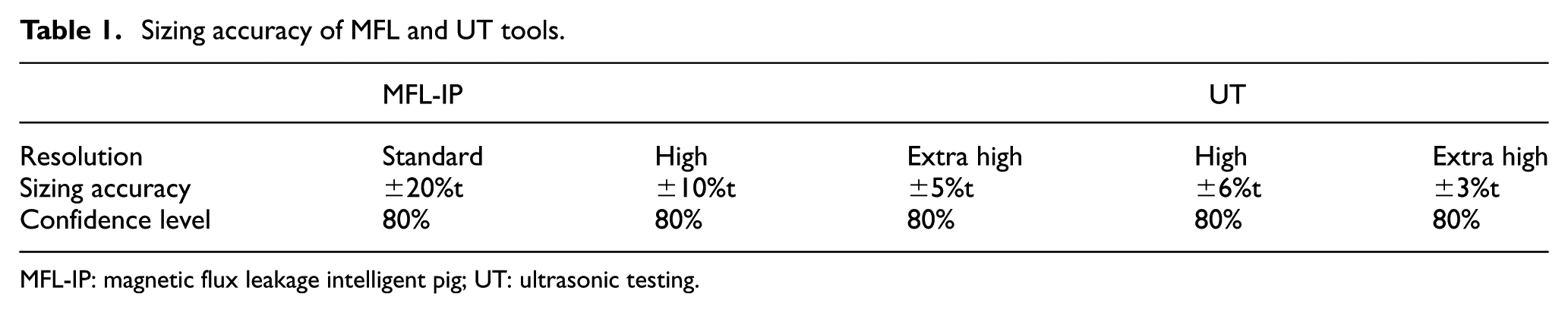
MFL-IP: magnetic flux leakage intelligent pig; UT: ultrasonic testing.

As shown in Table 1, the standard MLP-IP has a sizing accuracy of ±20%t with 80% confidence level. Although this error margin is significantly high, yet this standard resolution tool is preferred by most operators due to its comparatively low cost when compared to higher resolution techniques. This implies that the error in the measurements of the MFL-IP tool may cause an under- or over-estimation of the actual condition of the pipeline. This may result in operating a faulty pipeline or replacing a good one.

Different studies have been carried out to handle the error in ILI measurements. Yet, the majority of the suggested methods were parametric-based models. The simple least square regression (LSR) line was suggested by Hallen et al.¹¹ to calibrate the measurements of an ILI tool with some real field measurements. McNealy et al.¹³ proposed the API 1163 model for calibrating the error in corrosion measurements scanned with ILI tool with the field measurements. The assumption about corrosion measurements being normally distributed is required to apply such calibration. Average for tolerance calibration model was applied by Din et al.¹⁴ to estimate the calibrated corrosion rate of a certain pipeline using the corrosion data of three previous scans from different years. Caleyo et al.¹⁵ developed a statistical calibration method based on parametric regression estimators to calibrate the measurements of an MFL pig tools using the ultrasonic ILI-reported data and corresponding field measurements. The calibration process was based on comparing the growth of the pipeline defects using the readings of different tools as done by Salama et al.¹⁶ Others used the corrosion data from different scans at different times as done by Din et al.¹⁴ Abdolrazaghi et al.¹⁷ proposed the calibration of MFL-IP with the data of UT scan tool using the linear regression model. The calibration was done based on the readings of three runs of both MFL-IP and UT device. The error in ILI measurements was assumed to follow the normal distribution in order to perform the aforementioned calibration method.

Most calibration models used in the literature are of parametric nature. Parametric calibration models have a big limitation related to the normality assumption of the dataset. Although it is convenient for most researchers to use parametric models, it cannot cover all distributions of the measurement data. Non-parametric models, however, do not require the assumption of normality, thus, it can overcome the limitation of parametric estimators. Based on the previous discussion, this paper presents a non-parametric calibration procedure to reduce the error in the MFL-IP measurements using the UT readings. The procedure proposed in this paper was based on applying a weighted k-nearest neighbor (KNN) interpolation as a calibration tool. A new positioning approach was suggested to reduce the bias in the resulted measurements. The process was followed by a comparison of the effect of using various kernel functions and different positioning techniques on the measurements in order to get the closest, unbiased, and enhanced MFL corrosion measurements. The next section in this paper will present the statistical background behind the suggested method.

Statistical background

Interpolation can be defined as the prediction of an unknown or a missing value relative to a function or simply a sample point. The prediction is done by making use of the neighboring points that are known. Many different techniques can be applied, and some of these techniques are interpolators such as KNN interpolation, multivariate interpolation, bilinear interpolation, polynomial interpolation, quadratic interpolation, B-spline interpolation, bicubic spline interpolation, Gaussian interpolation, Lagrange interpolation, inverse distance weighting (IDW) interpolation and many others.^18–21 KNN interpolation has been used for time-series forecasting in several applications, such as coal-mill-related variables,²² electricity price predictions,²³ hydrologic time series,²⁴ in addition to image processing,¹⁸ data mining,²⁵ and big data classification.²⁶ In this paper, KNN interpolators were chosen to use the neighbor grid of the UT tool measurements in calibrating corrosion metrics of the MFL intelligent pig.

KNN interpolation can be defined as a statistical test conducted to determine a point significance in terms of its nearest neighbor contiguity. This is done to calculate the amount of deviation from the norm.^19,27 An estimation of the contiguity may be done using a weight function (also known as a kernel function), which is simply a function measuring the effect of every single neighbor point on the interpolated one. Simply, the value estimated of the required or missing point is the neighbor’s weighted average value.²⁸ The weight function must gain its maximum value at zero distance from the interpolated point, and as the distance increases, the function should decrease respectively.²⁹ The simplest weight function is described in Equation (1)^28,30

w_{i} = \frac{d_{i}}{\sum_{i = 1}^{n} d_{i}}; d_{i} = ‖ \hat{y} - y_{i} ‖

(1)

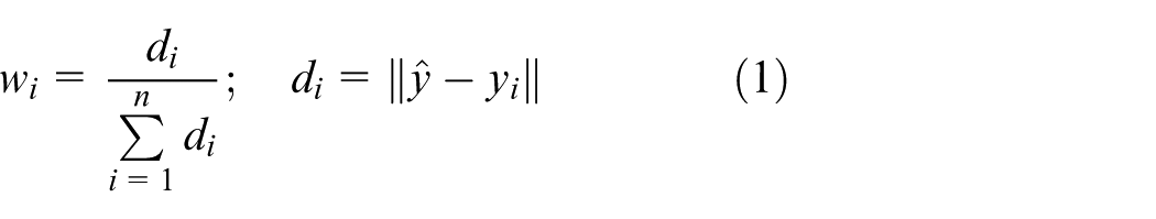
where $d_{i}$ is the Euclidean distance between two points defined by Equation (2)

d = ‖ x - y ‖ = \sqrt{\sum_{i = 1}^{n} {(x_{i} - y_{i})}^{2}}

(2)

where $x = (x_{1}, \dots, x_{n})$ and $y = (y_{1}, \dots, y_{n})$ , and $n$ is the vector size.^31,32

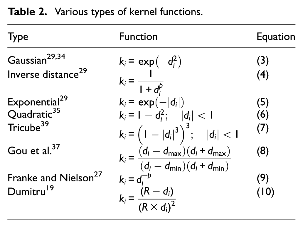
Various types of kernels can be found in the literature. The KNN weighted function was first introduced by Loftsgaarden and Quesenberry³⁰ in the field of density estimation. Similarly, Cover and Hart³³ introduced it for classification purposes. Hinton and Roweis³⁴ defined a stochastic neighborhood embedding algorithm used to visualize a given dataset by learning a low-dimensional embedding in two or three dimensions, based on the Gaussian kernel, Equation (3), introduced by Atkeson et al.²⁹ Wolberg used the inverse distance kernel to deal with a case of noisy data; the kernel is shown in Equation (4). In psychological models, exponential kernel, Equation (5), is used to give the weighted average for the model.²⁹ Fan and Hall³⁵ used the quadratic kernel introduced by Epanechnikov³⁶ as given in Equation (6). Wang³⁹ used the tricube kernel given in Equation (7). Gou et al.³⁷ combined the ratio between the query point and its farthest neighbor to the nearest neighbor distance. This ratio was made to introduce the kernel in Equation (8). Franke and Nielson³⁸ used a classic form of weight function as seen in Equation (9). Dumitru¹⁹ used a modified version of the weight function used by Franke and Nielson for superior results as shown in Equation (10). Table 2 shows the aforementioned kernels with their parameters of interest, where $p > 0$ is a power parameter chosen at random. $d \max / \min$ is defined as the distance between the farthest/nearest point and the interpolated point in the set. $R$ is the distance from the interpolated point to the farthest point of the set of data.

Table 2.

Various types of kernel functions.

Type	Function	Equation
Gaussian^29,34	$k_{i} = \exp (- d_{i}^{2})$	(3)
Inverse distance²⁹	$k_{i} = \frac{1}{1 + d_{i}^{p}}$	(4)
Exponential²⁹	$k_{i} = \exp (- \| d_{i} \|)$	(5)
Quadratic³⁵	$k_{i} = 1 - d_{i}^{2}; \| d_{i} \| < 1$	(6)
Tricube³⁹	$k_{i} = {(1 - {\| d_{i} \|}^{3})}^{3}; \| d_{i} \| < 1$	(7)
Gou et al.³⁷	$k_{i} = \frac{(d_{i} - d_{max}) (d_{i} + d_{max})}{(d_{i} - d_{min}) (d_{i} + d_{min})}$	(8)
Franke and Nielson²⁷	$k_{i} = d_{i}^{- p}$	(9)
Dumitru¹⁹	$k_{i} = \frac{(R - d_{i})}{{(R \times d_{i})}^{2}}$	(10)

The KNN algorithm interpolates the query point using Equation (11)

{\hat{y}}_{i} = \sum_{i = 1}^{n} w_{i} y_{i}

(11)

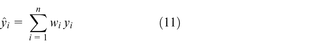
where $w_{i}$ is defined as the proper weight for every single one of $y_{i}$ neighbors to the query point $\hat{y}$ .²⁸

In this work, six kernels were used for calibrating MFL-IP corrosion measurements with the measurements of the UT device. The prediction behavior for the studied kernels was tested using two positioning approaches. The ordinary positioning practice (center position) assumes that the predicted point is located at the center of the neighbor grid (surrounded by the neighbor points as a rectangle or a circle). In the case of big neighbor grid, there is a possibility of overfitted prediction. Hence, a new positioning approach (moving position) was suggested. It is now assumed that the location of the predicted point is either next to the largest or the smallest point in the grid. The decision about the query point location depends on whether the value of the MFL-IP point is greater or less than the UT point.

Methodology

The corrosion data collected using two different devices have almost identical properties but may have a different design. For instance, the measurements that are collected using a UT scan device are given as a full grid of actual remaining wall thickness of the pipeline, respectively, to its length and circumference. However, the MFL-IP provides only corroded points in their exact positions along the length of the pipeline respective to their circumferential orientation. Hence, a mapping procedure is applied to join each point from the MFL-IP with its equivalent measure from the UT device, thus forming a pair.

Given the better sizing accuracy of the UT device compared to the MFL-IP, the UT device measurements were assumed to be the goal metrics and used for the calibration of the MFL-IP measurements. The KNN interpolation will be the basis of this calibration. Eight UT points are selected to set up a neighbor grid for the point that needs calibration. Figure 1 illustrates the position of the UT goal point with respect to the neighbors. 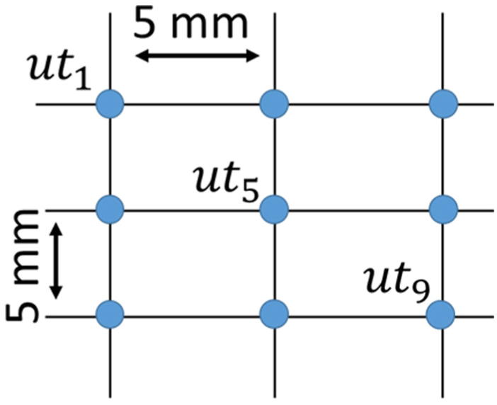The fifth element in the grid ( $u t_{5}$ ) represents the equivalent goal point to the MFL-IP measure that requires calibration. The calibration method proposed in this paper can be described as follows.

Figure 1.

UT neighbor grid.

The UT neighbor grid was expanded by inserting the MFL-IP measurements. Accordingly, the grid now consists of 10 elements instead of 9. Hence, the neighbors for the query point became 9 instead of 8. This number will be labeled as K, the number of neighbors in the model. The expansion was made using two approaches. The first approach is called the center position approach. This approach plants the MFL-IP measurements as the sixth element in each neighbor grid. The IP point was placed at a distance very near to the center of the grid, such that it is almost at the same position. 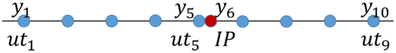Let ${y_{i}; i : 1, \dots, 10}$ be the response variable representing the expanded remaining wall thickness matrix, thus $y_{5}$ and $y_{6}$ represent the UT goal point and the IP point that require calibration, respectively, as shown in Figure 2.

Figure 2.

Remaining wall thickness expanded vector.

Since the IP point was placed as the nearest neighbor to the goal point, there will be a possibility of over-fitting or a biased estimation. In order to avoid this possibility a new positioning approach is proposed for the expansion. The proposed moving position approach takes into consideration the relationship between the original IP and UT measurements to avoid the possibility of over-fitting. An IP measurement is placed closest to the maximum point in the grid if it is greater than the UT measurement as shown in Figure 3(a).

Figure 3.

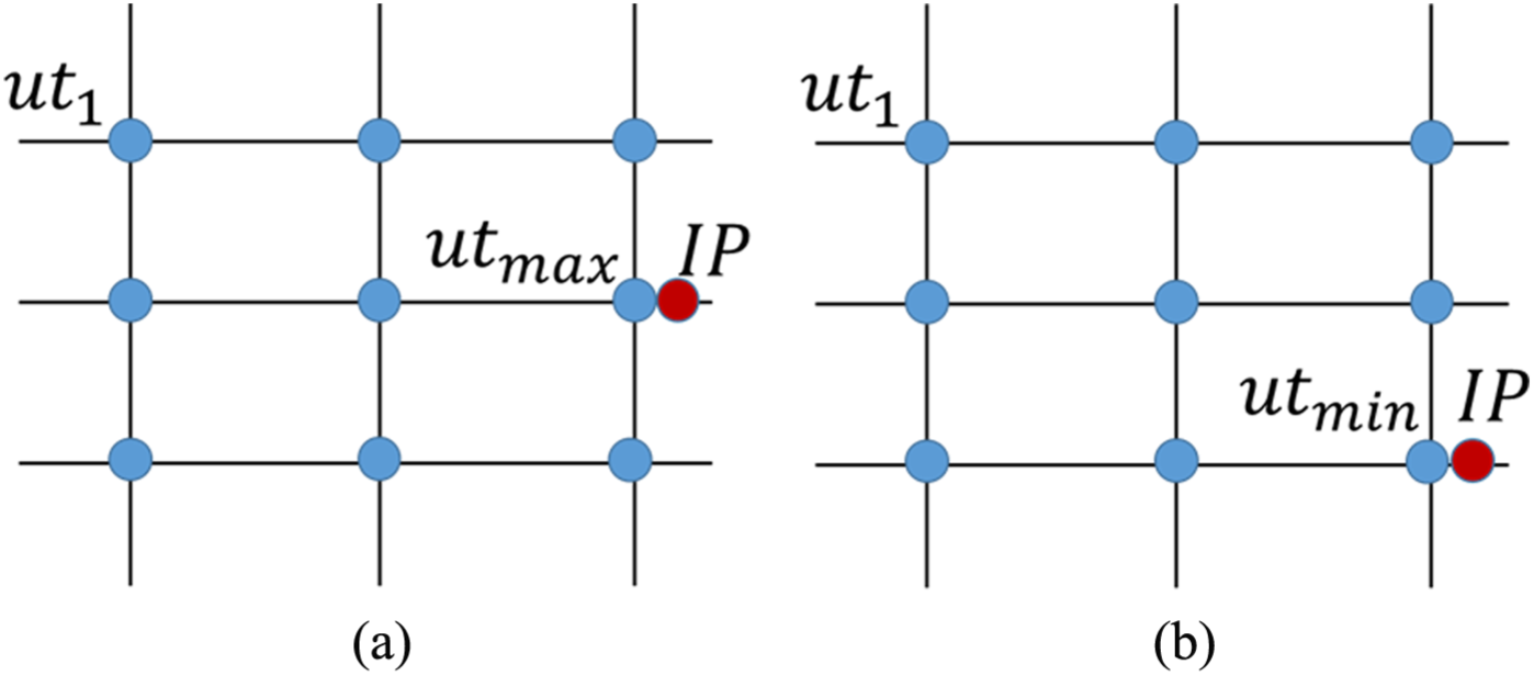
Expanded neighbor grid: (a) IP > UT; (b) IP < UT.

On the contrary, if MFL-IP measurement is smaller than the UT measurement, then the position of the point that requires calibration will be assumed to be the closest to the position of the minimum value point in the neighborhood, as shown in Figure 3(b). 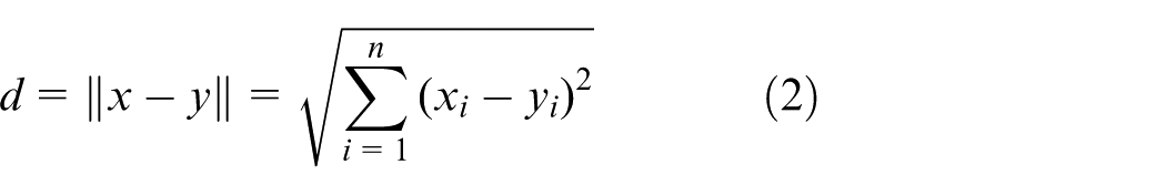This position will assure that the calibrated point will be relatively close to the original MFL-IP measurement rather than the goal measurement ( $u t_{5}$ ). This will reduce the possibility of a biased estimator.

The distance vector between the planted IP point and the other neighbors in the grid is generated using the Euclidean distance function expressed in Equation (2).

For the expanded vector, a weight sequence was calculated using the weight functions given in Table 2. The kernel function will concentrate on the closest neighbor to the IP point as it has the biggest effect on the estimation.

KNN interpolation (with k = 9 neighbors) is applied on the expanded vector. Equation (11) is used to replace the IP value with the weighted average calculated by the KNN interpolation. The result is labeled as the new enhanced MFL-IP corrosion measurements.

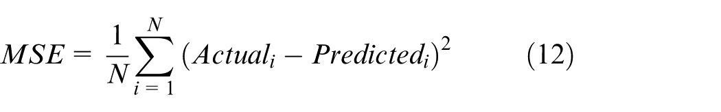
Mean square error (MSE) is used to evaluate the model’s performance and to point out the effect of using different kernels on the interpolation procedure for both approaches

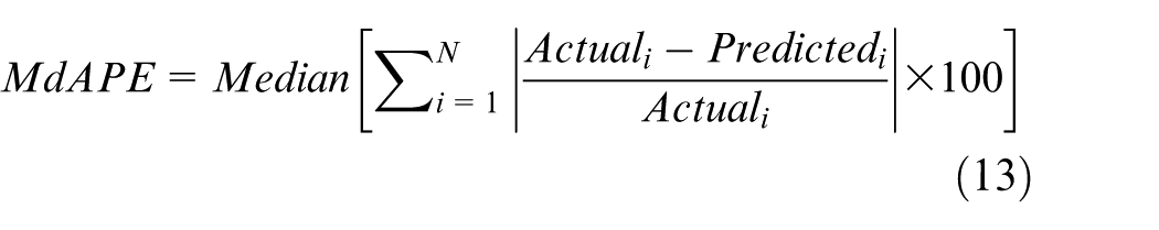
MSE = \frac{1}{N} \sum_{i = 1}^{N} {(Actua l_{i} - Predicte d_{i})}^{2}

(12)

This was followed by applying the median absolute percentage error (MdAPE) index to determine the preference of a certain kernel on the others. The usage of the median for the evaluation will increase the chance to find the superiority of one interpolator over the rest considering its ability in eliminating the effect of the extreme values (outliers) in the dataset⁴⁰

MdAPE = Median [\sum_{i = 1}^{N} | \frac{Actua l_{i} - Predicte d_{i}}{Actua l_{i}} | \times 100]

(13)

The bias of the model was measured by comparing the error in the estimated value from the original IP metrics using Equation (14) to ensure that the prediction model that depends on both suggested approaches is not over-estimating the measurements

Bias (\hat{ϑ}) = E (\hat{ϑ} - ϑ)

(14)

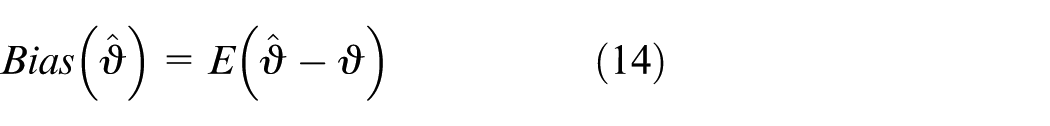
where $\hat{ϑ}$ is the approximated parameter and $ϑ$ is the original parameter. The approach with the less bias estimation compared to the original IP measurements will yield the best prediction.

Case study

This framework is applied to a set of corrosion data collected from oil pipeline used in Malaysia. It is about 20 years old and has a length of 3.9 km, a diameter of 25.4 cm, and an internal wall thickness of 12.7 mm. The data (depth, length, and width) of corrosion geometry parameters were collected using two ILI tools. An MFL-IP with a sizing accuracy of ±20% and UT scan device with a sizing accuracy of ±5%. Both suggested methodologies were applied to a section of the aforementioned pipeline that contained 273 corroded points.

Results and discussion

The results of applying the proposed methodology were illustrated at a single segment of the studied pipeline which contains 38 defected points. The calibration technique suggested in this paper show a remarkable enhancement in corrosion measurements for some of the used weight functions and a weak effort in others. The evaluation of the proposed interpolators was done by comparing the MSE and the MdAPE index for the first six of the suggested kernels as given in Table 2. The Franke–Nielson and Dumitru kernels contain a distance parameter at the denominator. Since the suggested methodology calculates zero distance between the center of the neighbor grid and the predicted point, both the abovementioned kernels will be resulted as infinity, making them inapplicable in this study due to the case of indetermination. The error evaluation was followed by a comparison of the difference between the original IP measures, the goal UT measures, and the interpolated measures. The measurement of the point with the thinnest wall thickness in the pipeline was compared between three cases: the actual metrics collected by UT device, the original metrics collected by MFL-IP device, and the enhanced metrics approximated using the proposed techniques.

Table 3 shows the error in the interpolated corrosion metrics using both the suggested methods for each one of the six kernels mentioned in Equations (3)–(8), indexed from A to F.

Table 3.

Mean square error (MSE) for interpolators.

MSE (mm)
Kernel	A	B	C	D	E	F
Center approach	0.093	0.092	0.094	0.095	0.104	1.129
Moving approach	0.145	0.124	0.151	0.288	0.265	0.502

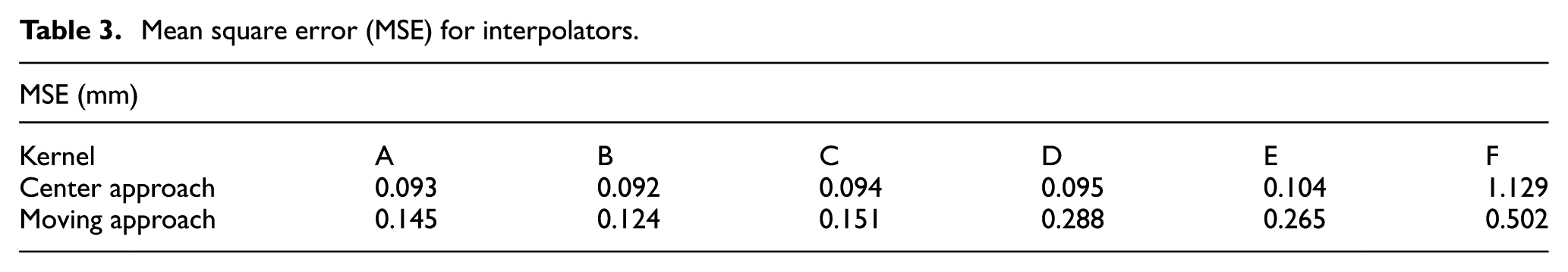
Based on the MSE values shown in Table 3, kernels A, B, C, and D have almost the same interpolating behavior when using the center position approach. Hence, the MdAPE index is calculated to determine the best among them as shown in Table 4.

Table 4.

Median absolute percentage error (MdAPE) for interpolators.

MdAPE (%)
Kernel	A	B	C	D	E	F
Center approach	1.68	1.61	1.75	1.73	1.95	5.38
Moving approach	2.18	1.99	2.26	3.23	3.06	4.30

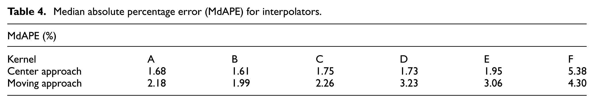
From the MdAPE index shown in Table 4, kernel B shows the best interpolating behavior with a MdAPE value of 1.61%, outperforming the accuracy of kernel A with 1.68%. Kernels C and D have almost the same interpolation abilities, while kernel F is seen to have the weakest effect between the studied kernels. This can be attributed to its unique definition that neglects the effect of the neighbors, given that the distance between the neighbor points in the grid when applying the center position approach is constant. However, when applying the moving position approach, kernels D and E show less accurate predictions (with errors of 0.288 and 0.265 mm, respectively) when compared to kernels A, B, and C with MSE values of 0.145, 0.124, and 0.151 mm, respectively. In the case of moving position approach, kernel B shows a much accurate prediction with 1.99% MdAPE index, followed by kernels A and C. Kernel E has a slightly better approximation when compared to kernel D with an MdAPE index of 3.06% and 3.23%, respectively. Kernel F has the minimal prediction accuracy compared to other kernels based on both MSE and MdAPE index.

Figure 4 presents a comparison between the original IP, goal UT, predicted center position approach, and predicted moving position approach line chart for all the studied kernels.

Figure 4.

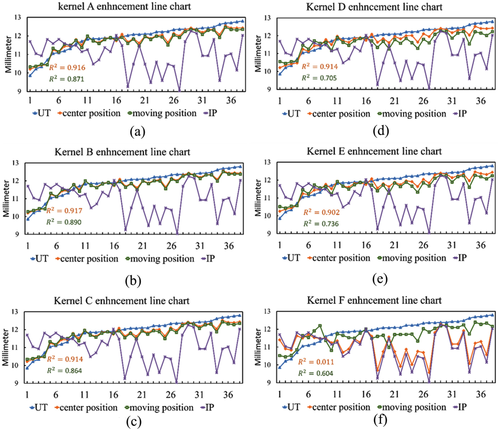
Comparison between original IP and goal UT for interpolators with different kernels.

It is clear from Figure 4 that kernels A, B, and C have prediction lines that are close to the goal UT measurements, which explains their small prediction error. It is also shown that the three kernels have very small differences as their line charts have almost the same alignment toward the UT line.

Table 5 shows the bias test for the studied kernels for both approaches. The error between the predicted and the original IP measurements was calculated using Equation (12) in order to study the bias of the predictors.

Table 5.

Bias of interpolators.

Bias
Kernel	A	B	C	D	E	F
Center approach	1.16	1.17	1.12	1.13	1.04	0.04
Moving approach	1.00	1.07	0.97	0.71	0.76	0.80

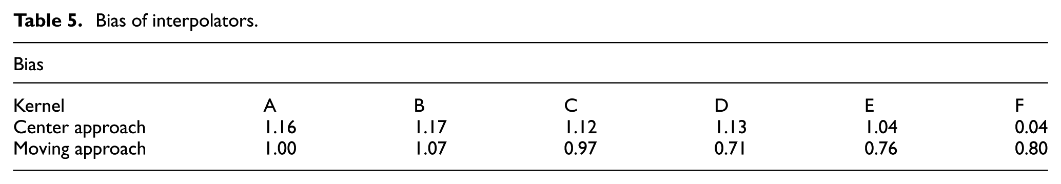
The method that has a smaller error when compared with the original IP measurements was considered less biased to the goal UT line. Hence, it is clear from Table 5 that the proposed moving position approach has a less biased interpolation behavior for all the kernels when compared to the center position approach. Thus, it is highly recommended to use the predicted measurements using this technique.

The economic benefit of such research can be clearly explained by analyzing the thinnest remaining wall thickness in the corroded pipeline. The point with the thinnest wall thickness in the pipeline is usually used in the extreme value analysis to determine the probability of system failure. Hence, the weakest part of the studied section was approximated using the suggested approaches to evaluate the calibration method as given in Table 6.

Table 6.

Thinnest wall thickness (mm) in the studied segment.

Original (IP)	Actual (UT)	Approach	Kernel
			A	B	C	D	E	F
11.70	9.86	CP	10.20	10.19	10.22	10.21	10.25	11.40
		MP	10.32	10.27	10.34	10.55	10.51	10.52

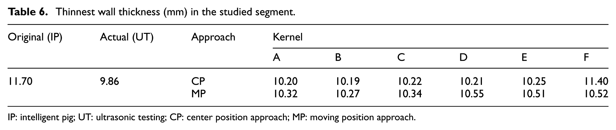
IP: intelligent pig; UT: ultrasonic testing; CP: center position approach; MP: moving position approach.

The MFL-IP operator reported that the thinnest part of the studied segment had a remaining wall thickness of 11.70 mm, while the reading of the UT tool showed that it should be 9.86 mm. This 1.84 mm difference between the two readings means that depending on the MFL-IP report, the pipeline can operate for an extra period of 4.6 years when compared to the reading of the UT tool, given that the average growth rate of the corrosion per year according to the NACE (National Association of Corrosion Engineers) is reported to be 0.4 mm.⁴¹ This under-estimation of the pipeline operating condition may lead to an unexpected system failure within the time frame given by the MFL-IP device. The enhanced measurements of the remaining wall thickness for the thinnest part of the segment were found to be as shown in Table 6.

Both approaches show a better approximation for the actual condition of the remaining wall thickness with an error that does not exceed 3% of the actual wall thickness recorded by the UT scan device. Considering the original sizing accuracy of the UT scan device, this means that the error in the estimated measurements is not more than 8% of the pipeline wall thickness. This result indicates a significant increment in the sizing accuracy of the corrosion metrics of the MFL-IP as the error was to be reduced from ±20%t to only ±8%t. Relative to pipeline operating lifetime, the enhancement in the MFL-IP metrics error will help to prevent a possible system failure for over operating the pipeline for 4.6 extra years.

As discussed earlier, most calibration methods used in the literature were of parametric nature. Hence, a comparison between the enhancement of the suggested approaches and the LSR line was done. The MSE of the LSR line was found to be 0.87 mm, which is way larger than the MSE for the KNN approach which was almost 0.1 mm when using kernel B for both positioning approaches. The enhancement of the thinnest recorded wall thickness using the LSR was found to be 10.93 mm, as shown in Table 7, but it was reduced to 10.19 and 10.27 mm using KNN approaches. There is almost 0.8 mm difference between the LSR and the KNN calibration methods, which means a difference of two extra operating years for the studied pipeline.

Table 7.

Thinnest wall thickness (mm): LSR vs KNN.

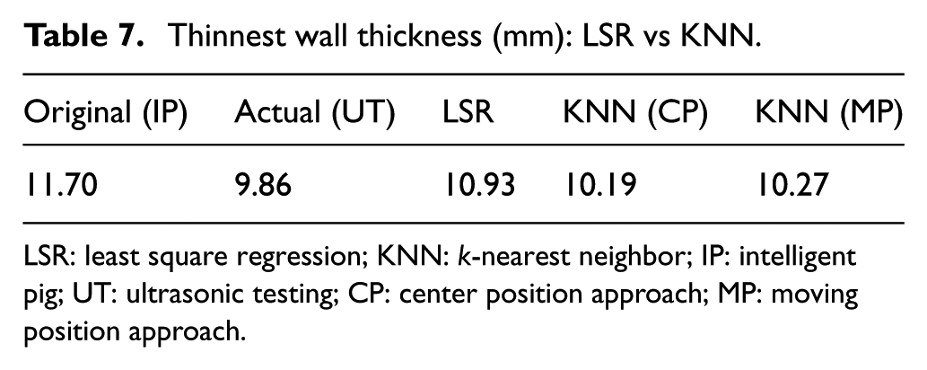
Original (IP)	Actual (UT)	LSR	KNN (CP)	KNN (MP)
11.70	9.86	10.93	10.19	10.27

LSR: least square regression; KNN: k-nearest neighbor; IP: intelligent pig; UT: ultrasonic testing; CP: center position approach; MP: moving position approach.

Conclusion

The proposed KNN interpolation method in this paper presented an effective calibration technique to enhance the sizing accuracy of the corrosion measurements collected by the IP tool. It has been shown that using the moving position approach will result in a less biased estimation when compared to the center position approach. The proposed technique enhanced the measurements of the IP tool to have an error that is not more than 8% of the pipeline’s wall thickness. This result is much reliable than the 20% affecting the IP device. It was concluded that using different kernels affects the KNN interpolation process differently. The inverse distance kernel showed the best interpolation behavior among the other studied kernels. However, the moving position approach showed a less biased estimation when compared to the center position approach with almost the same accuracy. The calibration of the thinnest wall thickness in the studied segment showed an under-estimation of 4.6 operating years, which can cause an unexpected system failure. The results indicate the potential of the proposed techniques in enhancing the corrosion measurements of pipeline corrosion NDT tools. Besides, the suggested KNN calibration showed a better enhancement behavior compared to LSR.

Footnotes

Acknowledgements

The authors would like to acknowledge the Universiti Teknologi PETRONAS for the financial assistance provided to conduct this research.

Declaration of conflicting interests

The author(s) declared no potential conflicts of interest with respect to the research, authorship, and/or publication of this article.

Funding

This research received no specific grant from any funding agency in the public, commercial, or not-for-profit sectors.

ORCID iD

Yaman Hamed

References

Central Intelligent Agency. The world Fact Book—Pipelines (km), https://www.cia.gov/library/publications/the-world-factbook/fields/2117.html (2013, accessed 20 April 2017).

El-Abbasy

Senouci

Zayed

, et al. Artificial neural network models for predicting condition of offshore oil and gas pipelines. Automat Constr 2014; 45: 50–65.

Noor

Yahaya

Ozman

, et al. The forecasting residual life of corroding pipeline based on semi-probabilistic method. J Civ Eng Sci Technol 2010; 1: 1–6.

Netto

Ferraz

Estefen

The effect of corrosion defects on the burst pressure of pipelines. J Constr Steel Res 2005; 61: 1185–1204.

Rathod

Anand

Ashok

Comparative analysis of NDE techniques with image processing. Nondestruct Test Eva 2012; 27: 305–326.

Zhang

G-M

Harvey

DM.

Contemporary ultrasonic signal processing approaches for nondestructive evaluation of multilayered structures. Nondestruct Test Eva 2012; 27: 1–27.

Jarvis

Cawley

Nagy

Current deflection NDE for the inspection and monitoring of pipes. NDT&E Int 2016; 81: 46–59.

Shukla

Karki

Application of robotics in onshore oil and gas industry—a review, part I. Robot Auton Syst 2016; 75: 490–507.

Pople

Wharf

. Magnetic flux leakage pigs or ultrasonic pigs? The case for combined intelligent pig inspections. In: Proceedings of the 6th international conference, pipeline rehabilitation and maintenance, Berlin, 6–10 October 2003, pp. 6–10.

10.

Beuker

Palmer

Quack

Inline inspection using combined technologies—magnetic flux leakage and ultrasonic testing and their advantages. In: Proceedings of the 4th pipeline technology conference, Hannover, 22–23 April 2009.

11.

Hallen

Caleyo

Alfonso

, et al. Statistical calibration of pipeline in-line inspection data. In: Proceedings of the 16th world conference on non-destructive testing, Montreal, QC, Canada, 30 August–3 September 2004.

12.

Beller

Reber

Schneider

. Tools, vendors, services-a review of current in-line inspection technologies. In: Proceedings of the pipeline pigging, integrity assessment, and repair conference, Houston, TX, 23 January 2002, pp. 23–24.

13.

McNealy

McCann

Van Hook

, et al. In-line inspection performance III: effect of in-ditch errors in determining ILI performance. In: Proceedings of the 2010 8th international pipeline conference, Calgary, AB, Canada, 27 September–1 October 2010, pp. 469–473. New York: ASME.

14.

Din

Ngadi

Noor

. Improving inspection data quality in pipeline corrosion assessment. In: Proceedings of the 2009 international conference on computer engineering and applications, Manila, Philippines, 6–8 June 2009.

15.

Caleyo

Alfonso

Hallen

, et al. Method propose for calibrating MFL, UT ILI tools. Oil Gas J 2004; 102: 76–76.

16.

Salama

Nestleroth

Maes

, et al. Characterization of the uncertainties in the inspection results of ultrasonic intelligent pigs. In: Proceedings of the 32nd international conference on ocean, offshore and arctic engineering, Nantes, 9–14 June 2013, pp. 9–14. New York: ASME.

17.

Abdolrazaghi

Hassanien

Cheng

. Relative statistical calibration of ILI measurements. In: Proceedings of the 2016 11th international pipeline conference, Calgary, AB, Canada, 26–30 September 2016. New York: ASME.

18.

Parsania

MPS

Virparia

. A comparative analysis of image interpolation algorithms. Int J Adv Res Comput Commun Eng 2016; 5: 29–34.

19.

Dumitru

Plopeanu

Badea

. Comparative study regarding the methods of interpolation. In: Proceedings of the 1st European conference of geodesy & geomatics engineering (GENG), Antalya, 8–10 October 2013.

20.

Olivier

Hanqiang

. Nearest neighbor value interpolation, 2012, https://arxiv.org/ftp/arxiv/papers/1211/1211.1768.pdf

21.

Lehmann

Gönner

Spitzer

. Survey: Interpolation methods in medical image processing. IEEE T Med Imaging 1999; 18: 1049–1075.

22.

Agrawal

Nag

, et al. Application of K-NN regression for predicting coal mill related variables. In: Proceedings of the 2016 international conference on circuit, power and computing technologies (ICCPCT), Nagercoil, India, 18–19 March 2016, pp. 1–9. New York: IEEE.

23.

Lora

Santos

JMR

Expósito

, et al. Electricity market price forecasting based on weighted nearest neighbors techniques. IEEE T Power Syst 2007; 22: 1294–1301.

24.

Lall

Sharma

. A nearest neighbor bootstrap for resampling hydrologic time series. Water Resour Res 1996; 32: 679–693.

25.

Kumar

Quinlan

, et al. Top 10 algorithms in data mining. Knowl Inf Syst 2008; 14: 1–37.

26.

Adeniyi

Wei

Yongquan

. Automated web usage data mining and recommendation system using K-Nearest Neighbor (KNN) classification method. Appl Comput Inform 2016; 12: 90–108.

27.

Franke

Nielson

, 1980. Smooth interpolation of large sets of scattered data. International journal for numerical methods in engineering, 15(11), pp.1691–1704.

28.

Härdle

Linton

. Applied nonparametric methods. Handb Econom 1994; 4: 2295–2339.

29.

Atkeson

Moore

Schaal

. Locally weighted learning for control (Lazy Learning). New York: Springer, 1997, pp. 75–113.

30.

Loftsgaarden

Quesenberry

. A nonparametric estimate of a multivariate density function. Ann Math Stat 1965; 36: 1049–1051.

31.

Weinberger

Blitzer

Saul

. Distance metric learning for large margin nearest neighbor classification. In: Weiss

Schölkopf

Platt

JC.

(eds) Advances in neural information processing systems. Cambridge, MA: MIT Press, 2005, pp. 1473–1480.

32.

Walters-Williams

. Comparative study of distance functions for nearest neighbors. In: Khaled

(ed.) Advanced techniques in computing sciences and software engineering. New York: Springer, 2010, pp. 79–84.

33.

Cover

Hart

. Nearest neighbor pattern classification. IEEE T Inform Theory 1967; 13: 21–27.

34.

Hinton

Roweis

. Stochastic neighbor embedding. In: Proceedings of the advances in neural information processing systems, 1 January 2002, pp. 833–840.

35.

Fan

Hall

. On curve estimation by minimizing mean absolute deviation and its implications. Ann Stat 1994; 22: 867–885.

36.

Epanechnikov

. Non-parametric estimation of a multivariate probability density. Theor Probab Appl+ 1969; 14: 153–158.

37.

Gou

Zhang

, et al. A new distance-weighted k-nearest neighbor classifier. J Inf Comput Sci 2012; 9: 1429–1436.

38.

Franke

Nielson

. Smooth interpolation of large sets of scattered data. Int J Numer Meth Eng 1980; 15: 1691–1704.

39.

Wang

Isaksson

Kowalski

. New approach for distance measurement in locally weighted regression. Anal Chem 1994; 66: 249–260.

40.

Shcherbakov

Brebels

Shcherbakova

, et al. A survey of forecast error measures. World Appl Sci J 2013; 24: 171–176.

41.

Caleyo

Valor

Venegas

, et al. Accurate corrosion modeling improves reliability estimations. Oil Gas J 2012; 110: 122–129.

Error-reduction approach for corrosion measurements of pipeline inline inspection tools

Abstract

Keywords

Introduction

Statistical background

Methodology

Case study

Results and discussion

Conclusion

Footnotes

Acknowledgements

Declaration of conflicting interests

Funding

ORCID iD

References