
Abstract
Background:
Temperature is one of the main variables need to be regulated in cryogenic wind tunnel to realize the true flight Reynolds number. A new control methodology based on L1 output feedback adaptive control is deployed in the temperature control.
Methods:
This design is composed of three parts: linear quadratic Gaussian baseline control, L1 adaptive control and nonlinear feedforward control. A linear quadratic Gaussian controller is implemented as the baseline controller to provide the basic robustness of temperature control. A L1 output feedback adaptive controller with a modified piecewise constant adaptive law is deployed as an augmentation for the baseline controller to cancel the uncertainties within the actuator’s bandwidth. The modified adaptive law can guarantee better steady-state tracking performance compared with the standard adaptive law. A global nonlinear optimization process is carried out to obtain a suboptimal filter design for the L1 controller to maximize the performance index. The nonlinear feedforward control is to cancel the coupling effects in control of the tunnel.
Results:
With these design techniques, the augmented L1 adaptive controller improves the performance of the baseline controller in the presence of uncertainties of dynamics. The simulation results and analysis demonstrate the effectiveness of the proposed control architecture.
Conclusion:
The modification of adaptive law plus the global nonlinear optimization of the filter in the L1 adaptive control architecture helps the controller achieve good control performance and acceptable robustness for the temperature control over a wide range of operations.
Introduction
Reynolds number is one of the main parameters used to evaluate the similarity between wind tunnel tests and true flight tests in aerodynamics. The cryogenic wind tunnel is a ground test facility which can produce flight Reynolds number by operating wind tunnel in cryogenic temperature with injection of liquid nitrogen. 1 In cryogenic wind tunnel, the Reynolds number is increased due to the increased gas density and decreased viscosity of the gas, and nitrogen behaves as a perfect gas at cryogenic temperatures. 2 At present, some cryogenic wind tunnels with high Reynolds number capabilities have been built in some well-known research institutes in the world, such as the DNW-KKK cryogenic wind tunnel in Köln, Germany; 0.3 m Transonic Cryogenic Tunnel (TCT) and the National Transonic Facility (NTF) at NASA in the United States; and the European Transonic Wind (ETW) tunnel in Germany.3,4
In contrast to regular wind tunnels, cryogenic wind tunnels have the ability to regulate Reynolds number, besides parameters such as Mach number and dynamic pressure. All the three flow parameters should be regulated accurately to obtain high-quality flow and aerodynamic test data for the test model. Because the Reynolds number is directly related to temperature in cryogenic wind tunnel, the temperature is one of the main parameters need to be controlled precisely over a wide range, which is regulated by injecting the liquid nitrogen into the tunnel and mixing with the circulating residential gas. The evaporation of injected liquid nitrogen would lower the gas temperature inside of the tunnel or balance the heat induced by other physical processes in the operation. It will be seen later that there exists a multi-variable, nonlinear and coupled dynamics for the three flow states. 5 Thus, a finely designed controller with reasonable robustness and good performance should be deployed in the automatic control of cryogenic wind tunnel to guarantee its smooth operations.
Because of the complex nature of cryogenic wind tunnel dynamics, some studies and researches on the development of control methodology for the tunnel had been carried out from the start of the concept of cryogenic wind tunnel decades ago, mainly concerning the modeling and control of cryogenic wind tunnel.6,7 Most of the researches have been conducted at the TCT, NTF of NASA Langley and ETW in Europe. Nonlinear gain-scheduled proportional–integral (PI) controllers with feedforward control were deployed in NTF in its early stages of operation. 2 A control algorithm with self-learning capabilities was designed and implemented in ETW. 3 Since then, some updates and re-innovation of the control system have been reported in recent years, 8 but without much details about its control designs seen from the published report.
The purpose of this paper is to deploy a new adaptive control method with guaranteed transient performance, L1 adaptive control, 9 to implement the control of cryogenic wind tunnel. Rather than considering the control of all three parameters, this paper mainly considers the temperature control in cryogenic wind tunnel.
L 1 adaptive control is a newly developed adaptive control methodology in recent years, mainly contributed by Cao and Hovakimyan.10–13 This new adaptive control has some distinguishing features compared with conventional adaptive controls, such as model reference adaptive control (MRAC). It can be viewed as a modified MRAC scheme, in which the basic architecture is based on the internal model principle. 9
The key feature of L1 adaptive control architecture is the guaranteed robustness in the presence of fast adaptation. In this adaptive architecture, the uncertainties in feedback loop can be compensated for only within the bandwidth of the control channel. 9 This leads to separation between adaptation and robustness in the adaptive law, and then desired and guaranteed transient performance for the closed-loop systems can be achieved. It can also guarantee bounded away from zero, time-delay margin (TDM). 11 Details of the theory can be found in Hovakimyan and Cao 9 and related papers on this issue.
With these features, the L1 adaptive control theory is suitable for the development of safety critical control systems. 14 L1 adaptive control in various forms has seen a lot of applications in many areas in recent years, especially in aerospace and flying vehicles.15–18 Moreover, L1 theory’s unique design procedures significantly reduce the tuning efforts required to achieve desired closed-loop performance, particularly in practical engineering and complex working conditions with the presence of various uncertainties and disturbances. 19 This is in contrast to the great challenges in tuning the conventional adaptive control system.
The main contribution of this paper lies in deploying a modified piecewise constant adaptive law in the L1 adaptive output feedback architecture, global nonlinear optimization design for the filter in L1 control structure and the application of L1 adaptive control in cryogenic wind tunnel.
The paper is organized as follows. Section “Dynamic model of cryogenic wind tunnel” gives a brief introduction of the facility, presents the nonlinear dynamics of cryogenic wind tunnel and the linear temperature model at nominal condition. Section “Controller design” discusses the controller design and its main components. Section “Simulation results and analysis” gives the simulation results and analysis. Section “Conclusion” concludes the paper.
Dynamic model of cryogenic wind tunnel
Facility description
The facility considered in this paper is a closed-circuit, pressurized, outer thermal-insulated small cryogenic wind tunnel. The schematic diagram is shown in Figure 1.
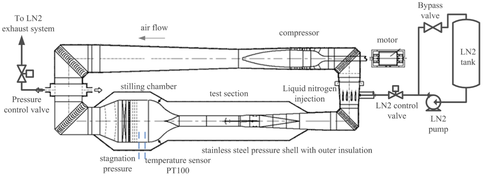
Schematic diagram of cryogenic wind tunnel.
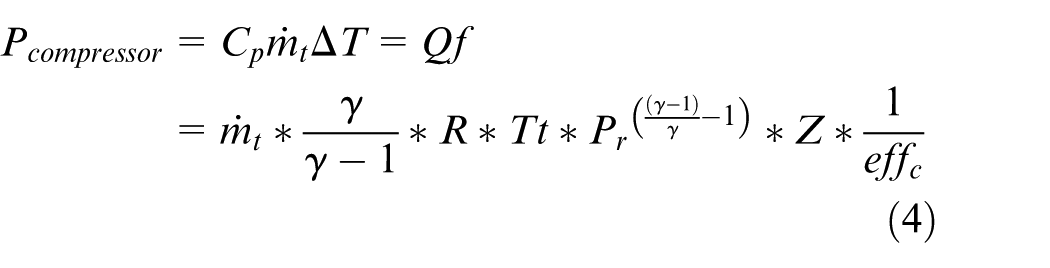
A compressor driven by electrical motor moves nitrogen gas around the circuit. When in operation, the liquid nitrogen is injected into the tunnel at the upstream of the compressor to evaporate and mix with the gas inside of the tunnel. The gas nitrogen inside of the tunnel is extracted to the LN2 exhaust system by the pressure control valve, which is located at upstream of the stilling chamber. The main operation parameters, which are total pressure, total temperature and Mach number in test section, need to be controlled precisely within the whole operation envelop. The operation range is 110–300 K for total temperature, 1.15–4.5 atm for total pressure and 0.15–1.2 for Mach number.
Normally, the operation of cryogenic wind tunnel starts with a cooling-down process from ambient temperature. To keep the tunnel structure thermal stress within certain limits, there is a temperature change rate constraint during the process. After the temperature set point is reached, quick changes of test section states will be carried out for the test. When test is finished, a temperature-rising process with rising rate limitation will occur before the end of entire operation.
Because the wind tunnel metal wall is wrapped within the outer insulation layer, and its internal surface has a direct contact with the gas in the tunnel, there exist heat exchanges between the wall and the gas when the gas temperature goes through some changes, and there is no net heat exchanges between the two when the temperature of tunnel is in balance. Due to the massive weight of metal tunnel wall, which leads to the massive heat inertia in the system, this heat exchange has considerable impact on the temperature dynamics of the tunnel. The existence of the wall heat inertia acts as a big damper and stabilizer when the gas temperature changes in the tunnel.
The temperature is measured by a specially designed PT100 resistance temperature detector (RTD) sensor, with high precision and quick response. Due to the circulating of the nitrogen gas in the circuit, from start of any variation of liquid nitrogen injection, there will be a delay before the RTD sensor can sense any substantial temperature change. The delay would be varied according to the flow rate in the circuit.
The mass volume of liquid nitrogen injected into wind tunnel is regulated by LN2 control valve, and its opening corresponds to the LN2 injection area, which then directly relates to the LN2 injection mass volume with assumption of constant pressure from the LN2 pump supply.
Dynamic model of the cryogenic wind tunnel
The modeling of the tunnel dynamics mainly follows the study of Balakrishna et al., 2 and the dynamics will briefed here for the completeness of the paper.
First, some basic parameters of the wind tunnel are defined as
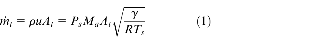
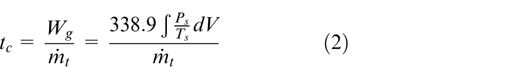
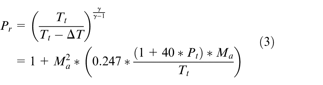
where
The main state dynamics is given as
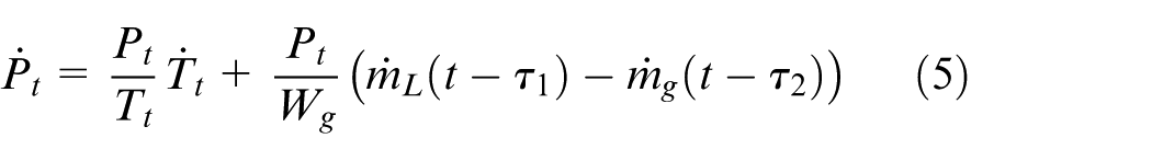
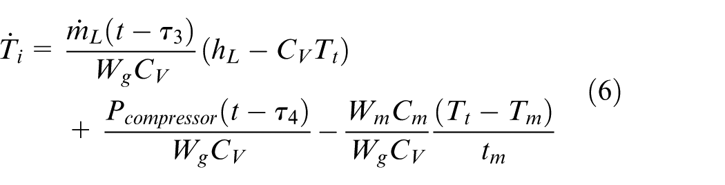
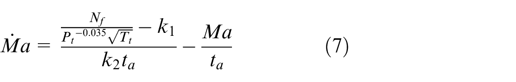
where
The nonlinear dynamics will be used for derivation of linear temperature dynamics and used as full cryogenic wind tunnel dynamics.
Linear model for temperature control
Linear approximation of the temperature dynamics will be utilized for designing the controllers and analyzing the closed-loop system.
From Equation (6), it is seen that, when the tunnel is at equilibrium state, there is no temperature difference between the tunnel wall and the gas. So the heat generated by the compressor is offset by the cooling capacity of the injected liquid nitrogen mass flow
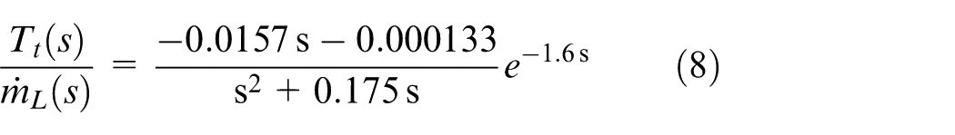
When approximating temperature dynamics with linear model, regular system identification tool is used at certain operation point of the nonlinear model. Because the identification process is a routine, it will not be covered here in detail. The identified linear temperature model at an equilibrium point, Pt = 200 kPa, Tt = 150 K, Ma = 0.5, is given as below, with all values non-dimensionalized
The compressor-induced heat effects on the temperature dynamics can be considered as equivalent negative liquid nitrogen input in this linear model. In this case, it is assumed as
Figure 2 shows the comparison of step responses of linear temperature model and nonlinear model, subjected to the same 2.5% liquid nitrogen step change at an equilibrium point. The goodness of fit is 98.85% in normalized root mean square error (NRMSE) measure.
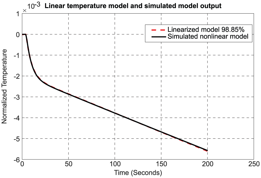
Response comparison of linear and nonlinear temperature model.
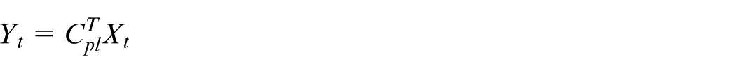
The state-space form of Equation (8) is given as
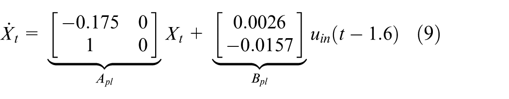
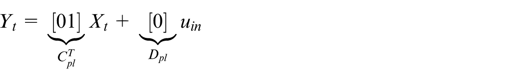
where
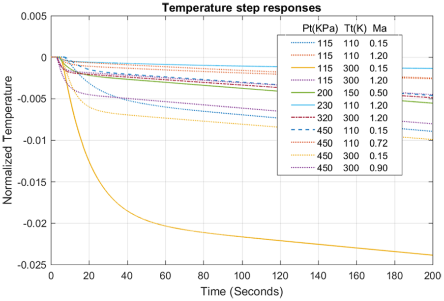
Temperature responses at typical points subjected to 2.5% LN2 step input.
Because temperature command change at one time is relatively small compared with the whole temperature range, and the total pressure,
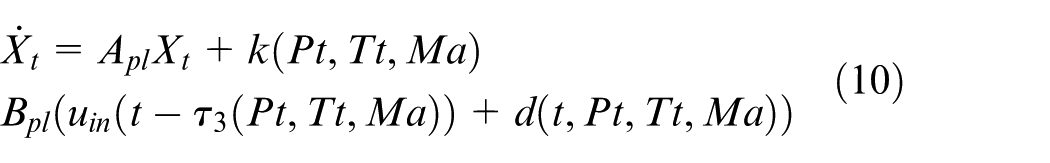
where Apl∈R2×2, Bpl∈R2×1,
Controller design
The control objective is to ensure that the gas temperature tracks a desired reference trajectory with some performance bounds. The controller should compensate for the nonlinear uncertainty and disturbances over a wide range of wind tunnel operation. The general design approach is to design a robust optimal linear controller as baseline controller, and then an adaptive controller is deployed as an augmentation to the baseline controller.
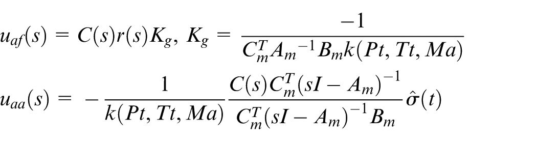
The baseline controller is implemented as a linear quadratic regulation (LQR) optimal controller with help of a Kalman filter, which is known as linear quadratic Gaussian (LQG) controller.20,21 Then, it is augmented by a L1 adaptive controller. A nonlinear feedforward controller is used to neutralize the effects of the induced heat generated by compressor. The overall control signal can be expressed as

where
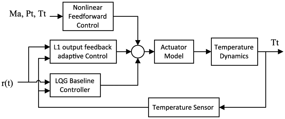
Block diagram of temperature controller.
The L1 adaptive control theory provides flexible architectures for wide-range classes of system. 9 In our case, the L1 adaptive output feedback control with the piecewise constant adaptive law22,23 is chosen as the adaptive structure with the presence of time-varying unmatched uncertainties. 24
Duo to the wide range of temperature control, the LQG baseline controller and L1 adaptive controller are all gain scheduled according to the states of the tunnel. The following sections mainly focus on controller design for the nominal condition in Equation (9), and gain scheduling will be illustrated in the design.
LQG baseline controller
As the implementation of LQG is outlined in Cao and Hovakimyan, 22 only an overview of the derivation is presented.
LQR optimal controller
The nominal closed-loop system should have appropriate pole locations to guarantee the control response, steady command tracking performance and proper stability margin. For this system, integral is needed to form the state-feedback controller. The states in Equation (9) are augmented with integrated temperature tracking error,
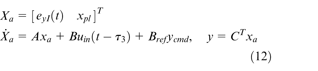
The controllability for the extended pair of matrices (A, B) is preserved if the original pair (Apl, Bpl) in Equation (9) is controllable.
20
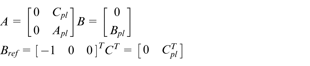
An optimal state-feedback gain matrix KLQR is obtained by solving the algebraic Riccati equation (ARE) associated with Equation (12), then the control law,
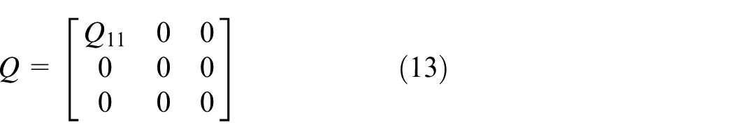
which penalizes the first state of Equation (12), the integrated tracking error. The Q11 is left as a parameter, which could be used to tune the closed-loop dynamics. It can be checked that the pair (A, Q1/2) is observable when Q11 is not 0. With the problem here, the value is chosen as Q11 = 0.95, and the optimal feedback gain is obtained as KLQR = [ –0.9747 –60.5725 –15.2129].
In the LQR design above, the delay
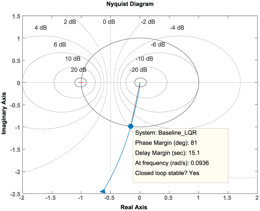
Nyquist plot of the nominal controlled system.
It is seen from Figure 5 that the TDM is about 15.1 s, much larger than the maximum possible time delay in the system. This is to maintain satisfactory control performance when the maximum time delay happens in temperature control. Linear analysis shows that the closed-loop temperature dynamics is mainly dominated by poles λ1,2 = [−0.1287, −0.1182], and their damping ratios are all 1.
The baseline controller at other operation points can be expressed as ub = KLQR*Xa/
Kalman filter
The LQR controller needs all the states in Equation (9) to be measurable to form the optimal state feedback. While only temperature can be measured in the system, a Kalman filter as below is used to estimate the unmeasurable state in Equation (9)

where L(t) is the Kalman filter observer gain and
L 1 adaptive output feedback control with modified piecewise constant adaptive law
The L1 adaptive output feedback controller augments the LQG baseline controller to compensate the uncertainties when the closed-loop system deviates from the nominal condition. Unlike MRAC, L1 adaptive control compensates the estimated uncertainties only within the bandwidth of an integrated low-pass filter in L1 control structure. 12 Normally, the low-pass filter bandwidth would match the bandwidth of the actuator in the system and should not go beyond it. The filter ensures that the control signal remains in low-frequency in presence of fast adaptation and large reference inputs.9,24
The underlying theory and its accompanying mathematical proofs for L1 adaptive output feedback control are detailed in previous works.9,22,25 An architectural overview is given in Figure 6. The closed-loop plant in the figure includes the baseline controller.
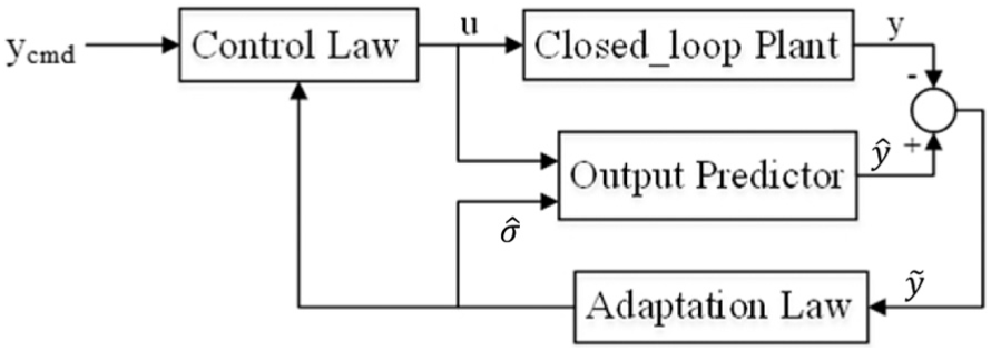
Block diagram of L1 adaptive output feedback controller.
Plant dynamics in L1 adaptive output feedback control framework
As mentioned above, when the system is closed by the LQG baseline controller, the temperature dynamics is dominated by closed-loop poles λ1,2 = [−0.1287, −0.1182]. This is the nominal closed-loop control behavior. Thus, the transfer function M(s) = C1 /((s−λ1) (s−λ2)) can be used to represent the new closed-loop system characteristics, where C1∈R is a constant. Let Am∈R2×2, Bm∈R2×1 and
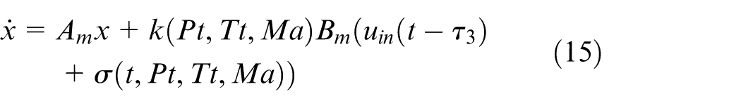

where
There are some assumptions about the uncertainties and disturbances term
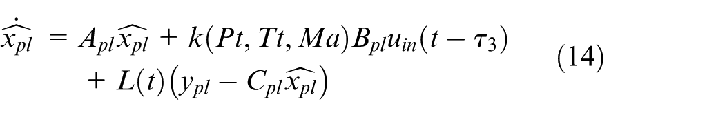
Output predictor
The output predictor in Figure 6 represents the desired closed-loop system behavior M(s) plus the estimated uncertainties. With incorporation of actuator dynamics in the output predictor17,26 and delay
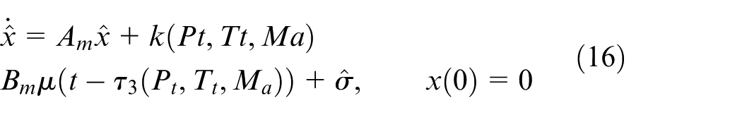
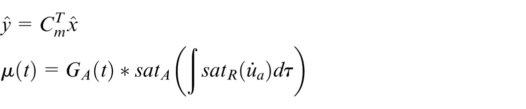
where
Modified piecewise constant adaptation law
The piecewise constant adaptive update law for

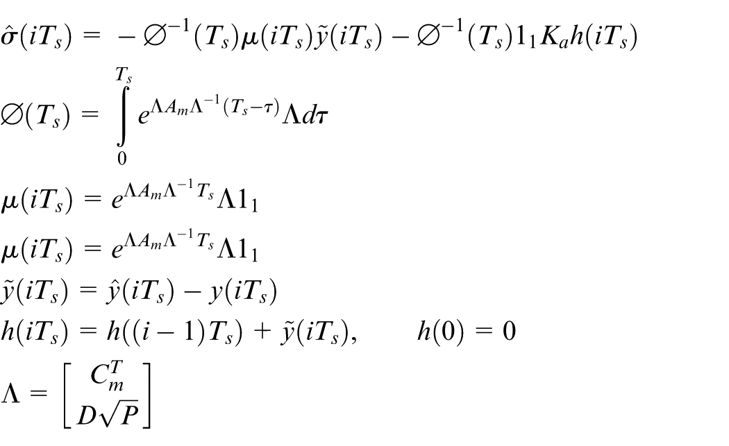
where

and D in
Remark 1
The main difference of this adaptive law compared with the standard form in Hovakimyan and Cao
9
and Lavretsky and Wise
20
lies in the extra term
Control law
The control law is given as

where C(s) is designed to ensure that C(s) has unity DC gain, and the
The feedforward term
Only the uncertainty compensation part
Stability condition and performance bounds
According to L1 adaptive control theory, the reference system corresponding to Equation (16) is given as

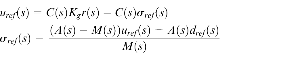
where A(s) is the nominal model with respect to the L1 controller, and

hold uniformly for t > 0. The values of L and L0 are supposed to be known.
Because the original plant is closed by the baseline LQG controller, and the L1 adaptive controller maintains the nominal closed-loop behavior under uncertainties, in this case,
The sufficient L1 norm stability condition for the reference dynamics in Equation (19) is derived in Hovakimyan and Cao 9 and Lavretsky and Wise 20 as

where
With the L1 norm stability condition (20) holds, it is proved that the following performance bounds between the L1 closed-loop adaptive system and its corresponding reference system hold
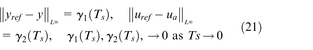
where
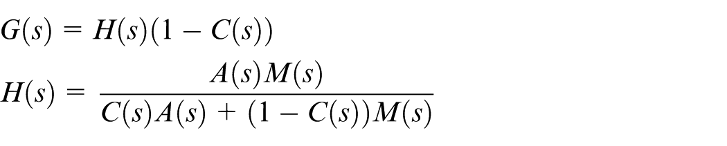
Filter design through global nonlinear optimization
In L1 adaptive control, the filter C(s) would determine the tradeoff between performance and robustness. Normally, the higher the bandwidth of filter C(s), the better the control performance, but with less robustness for closed-loop system. For temperature control here, with proper TDM guaranteed, making the L1 norm
When formulating the nonlinear optimization problem, the following analysis model is used for computation of delay margin and L1 norm.
The L1 adaptive output feedback controller could be approximated by a linear disturbance observer according to the study of Kharisov et al. 27 Then, the linear system theory is used to formulate the constraints and cost functions in the optimization problem. The Kalman observer in baseline controller will not be considered in the analysis because it is designed only affecting high-frequency behavior.
Then, the optimal filter design here is the solution of the constrained nonlinear L1 norm minimization problem stated as

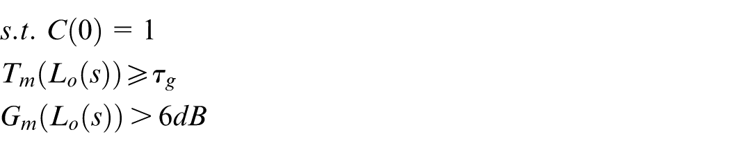
where
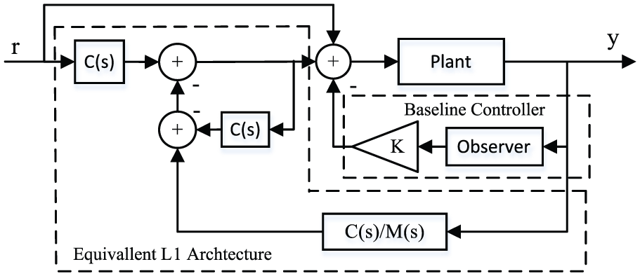
Equivalent linear architecture for the L1 adaptive augmented controller.
For the system here, a three-order filter with relative degree 2 and unity DC gain is chosen as
Comparison of filters.
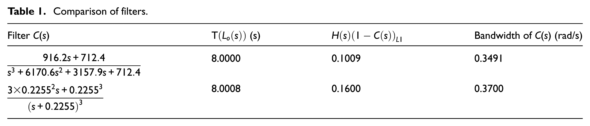
The suboptimal filter above is designed for the nominal case of Equation (9). It can be verified that the resulting filter is also a suboptimal design for other operation points of the wind tunnel, guaranteeing the same TDM when deploying the gain-scheduling LQG baseline controller and L1 adaptive controller, because the L1 norm is proportional to the dynamic gain of
Implementation issues
The Am, Bm and Cm in output predictor (16) are given as
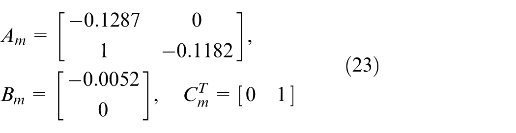
The choice of
In L1 adaptive control with piecewise constant adaptive law, the inverse of the sampling time Ts is equivalent to the adaptive gain. 24 So, the Ts should be set as low as possible within the available computing power. In this case, a sampling time of Ts = 0.02 s is suitable. Higher sampling rate has not been found to improve the performance significantly in simulation.
Nonlinear feedforward controller
From Equations (3)–(7), it is seen that the control of Mach number has coupling effects on temperature control. This effect can be expressed and modeled with good approximation in wind tunnel, and the needed liquid nitrogen mass injection to compensate that heat variation can also be estimated. 2 Thus, the nonlinear feed forward controller can be formulated as
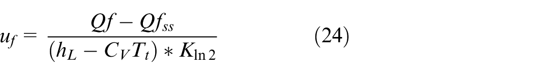
where
Because of the good approximation of coupling effect, this feedforward control law will only produce small uncertainty for the closed-loop system and will not cause stability problem, provided that the L1 augmented controller has enough stability margin.
This nonlinear feedforward controller can offset the coupling effects caused by the Mach number control and large pressure variation. This will be shown in the next section.
Simulation results and analysis
Most of the simulations are initialized with the same controller designed at the nominal condition without gain scheduling to show the robustness of the controller. For comparison, a conventional PI controller with comparable closed-loop control bandwidth is formulated, and its simulation results will be presented in some cases.
In simulations, the actuator dynamics for liquid nitrogen injection control valve is assumed to be
Control law to be compared
A classical PI controller is designed with the nominal linear temperature model by deploying classical linear control design method to attain the same control bandwidth and phase margin as that of the ideal LQR controller in section “Controller design.” The PI controller is given as
It is verified that controlled systems with the PI controller and ideal LQR controller all have the same bandwidth of 0.0936 rad/s, and the same phase margin of 81°.
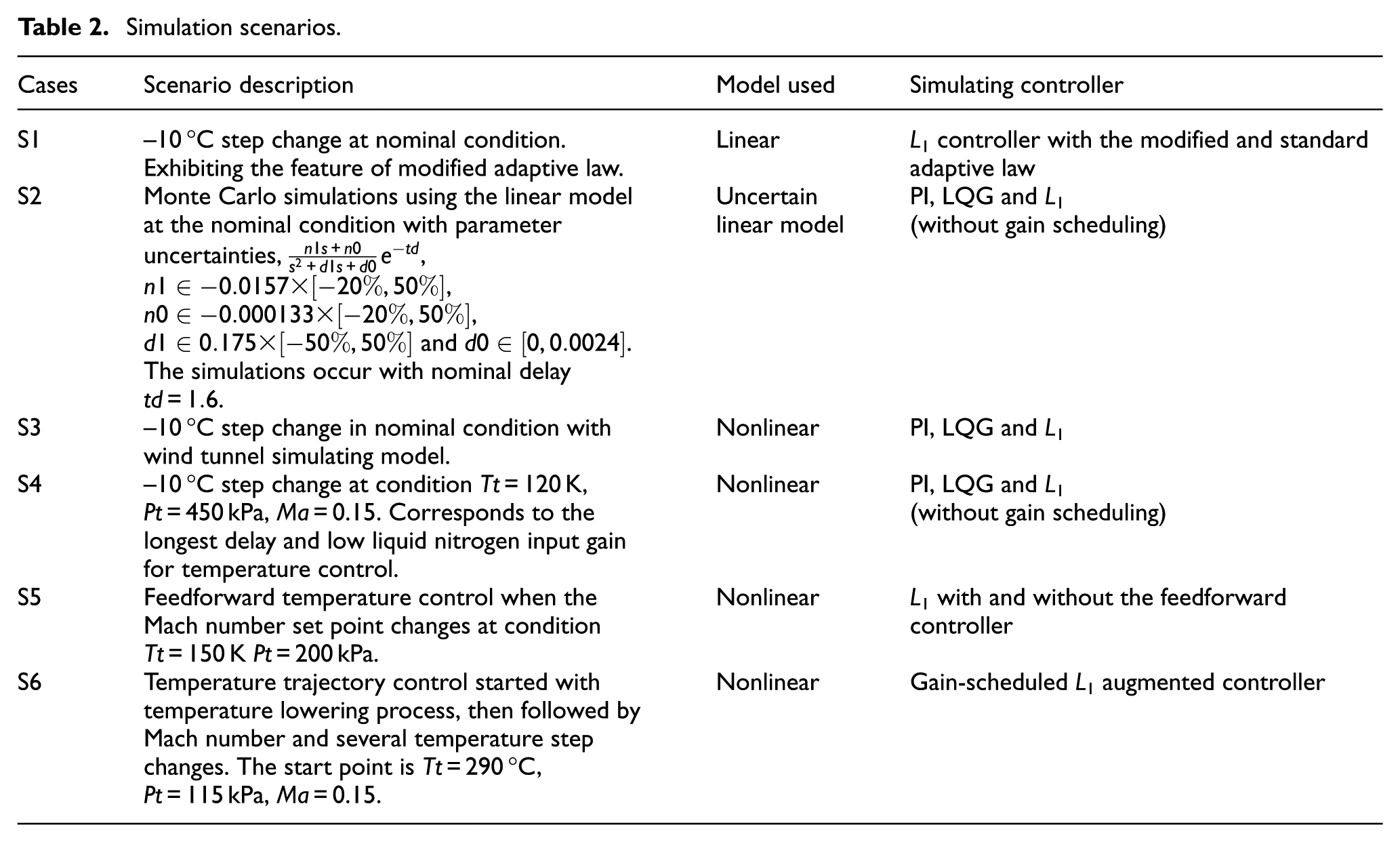
Simulation scenarios
All simulation scenarios are outlined in Table 2. In the table, L1 means the L1 augmented controller.
Simulation scenarios.
Results and analysis
Figure 8 shows −10 °C temperature set point change controlled by L1 augmented controller with standard and modified adaptive laws, respectively. Both temperature responses have similar transient performance, but the L1 controller with modified adaptive law has better steady-state tracking performance. This is because this modification can deliver better estimation of the uncertainty, and then the output predictor follows the reference model (20) better.
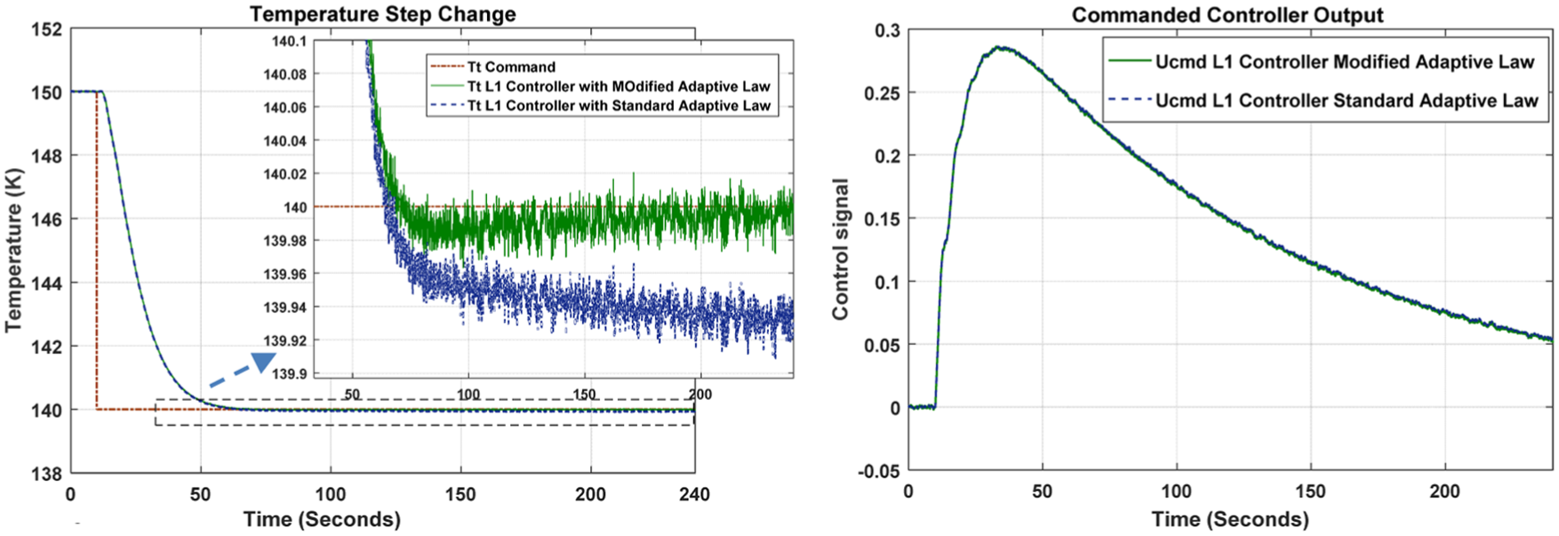
–10 °C step change at nominal condition with different adaptive laws (S1).
Figure 9 shows that the Monte Carlo runs with the uncertain linear model to examine the performances of the three controllers. The uncertainties mainly cover parameter uncertainties, and the ranges of the uncertainties can characterize possible parameter variations at operation points. This result shows that the LQG baseline controller and L1 augmented controller have much better control performance than the conventional PI, and the L1 augmented controller outperforms the LQG baseline controller. In some cases, the control signal of the L1 augmented controller signal exhibits some jittering to sustain the appropriate response of the temperature. This will be explained later in the robustness analysis.
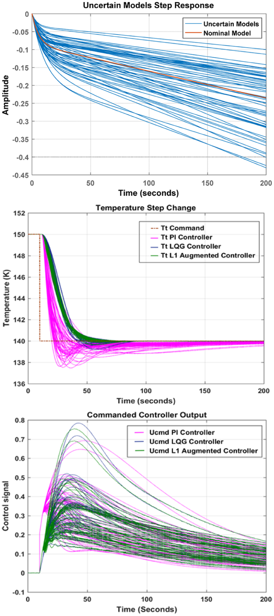
–10 °C step change in Monte Carlo simulations with uncertain linear model (S2).
The scenarios S3–S6 are with nonlinear cryogenic wind tunnel model. S3–S6 use the same nominal L1 augmented controller without any retuning. In most cases, the actuator output are presented in controller output figures.
Figure 10 shows the temperature responses of all three controllers at the nominal condition. The LQG baseline controller and L1 augmented controller have similar performance like that in S1, better than the conventional PI controller.
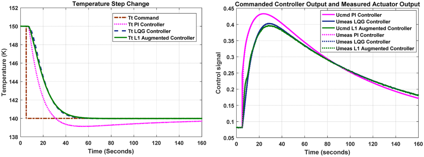
–10 °C step change in nominal condition with nonlinear simulation model (S3).
Figure 11 presents the temperature control with the longest delay of about 4.16 s, which happens at Tt = 120 K, Pt = 450 kPa, Ma = 0.15. It shows that the L1 augmented controller retains the basic tracking characteristics of nominal case, while the LQG controller and PI controller exhibit much larger overshooting, and obvious temperature oscillation can be observed in LQG controller results.
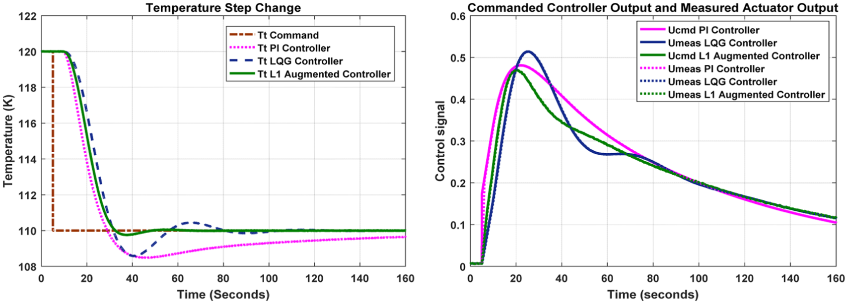
–10 °C step change at Tt = 120 K, Pt = 450 kPa and Ma = 0.15 with nonlinear simulation model (S4).
It can be seen from the results of S3–S4 that the actual actuator output can follow the controller signals well for L1 augmented controller and LQG controller. While for PI controller, because of the existence of direct P control, the actuator output can hardly follow the command signal at the beginning of temperature command changes. In some cases, this would lead to deteriorated control performance.
Figure 12 shows the nonlinear feedforward temperature control when Mach number undergoes changes. It is seen from the controller output that the feedforward controller compensates the temperature variation in advance before the temperature feedback can reflect the error signal. The compensation signal has some advance compared with that of the case with feedback controller only. So the temperature variation induced by the Mach number control is greatly reduced. It shows the effectiveness of the temperature feedforward controller.
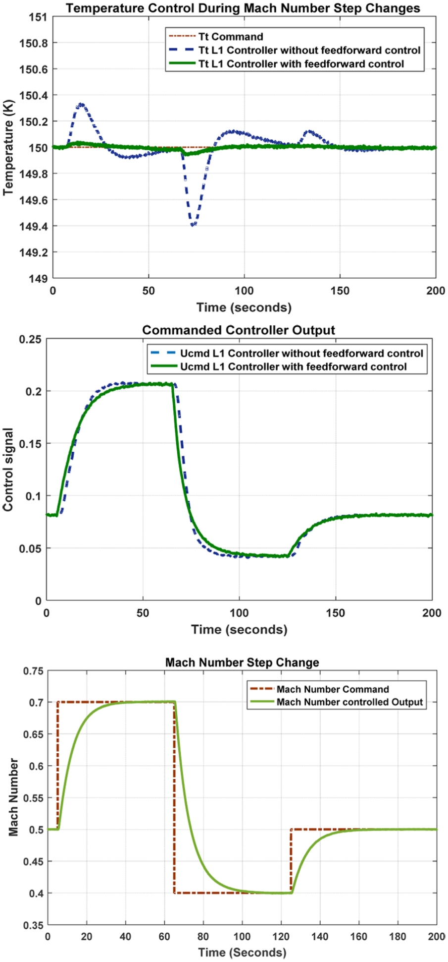
Feedforward temperature control during Mach number step changes (S6).
The simulation result shown in Figure 13 corresponds to regular cooling-down process and a typical temperature control process in cryogenic wind tunnel operation. The ramp change of temperature corresponds to temperature-lowering process, where the temperature does not need to track the temperature target command exactly. The ramp slope is used to constraint the temperature change rates. After total temperature reaches the first destination 160 K, Mach number is controlled to 0.6 from 0.15, at the time of 850 s. The temperature feedforward controller is in effect at this point to prevent the temperature from large variation. Then, the temperature goes through several step changes, including one temperature rise step change. The temperature can follow the command well. The wind tunnel metal wall temperature, which is also shown in the figure, follows the gas temperature in the trends. The controlled Mach number shown in the figure followed its command well. It is normal to see some deviation from its set point on the curve of Mach number when the temperature undergoes sharp changes, because the Mach number is closely related to the temperature of gas. The total pressure would vary with the variations of liquid nitrogen injection and gas temperature, but it is maintained close to the set point, 115 kPa, in the entire process. The gain-scheduled L1 augmented controller is deployed in this case.
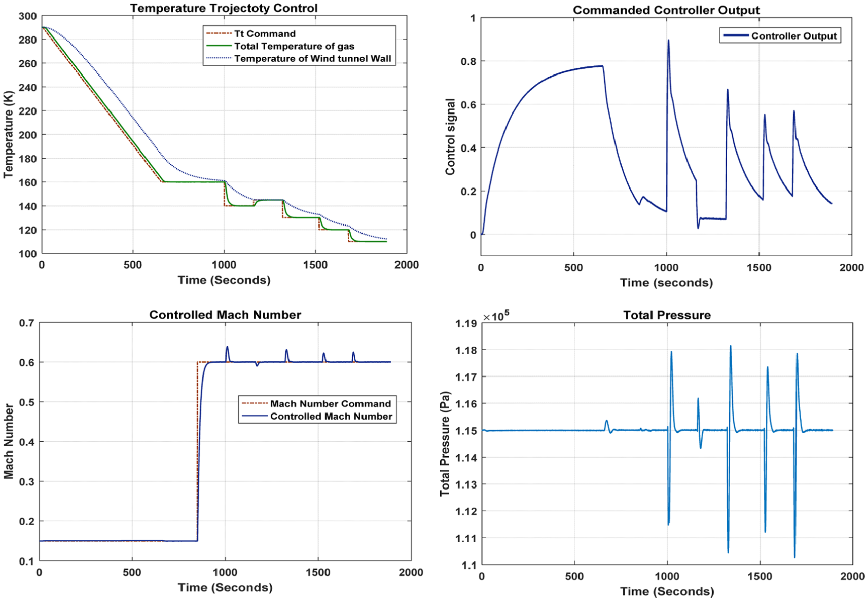
Temperature trajectory control in normal cryogenic wind tunnel operation (S7).
Robustness analysis
As mentioned above, the L1 adaptive controller with piecewise constant adaptive law can be approximated by disturbance observer or a linear time invariant system as long as the sampling time Ts is small, according to the study in Kharisov et al. 27 Thus, linear analysis methods can be used to assess the robustness of the closed-loop system. When proceeding the analysis, it is assumed that the actuator model’s rate and position are not saturated, and the actuator dynamics is ignored for its relative wider bandwidth compared to the plant dynamics. The state observer dynamics in the LQG baseline controller is not included in the model to simplify the analysis, because the observer is designed not to affect the low frequency response of the system.
The feedback system is analyzed using the input loop transfer function with the nominal linear temperature model. It is a scalar, open-loop transfer function from the actuator input of the plant to the output of the controller, which can be derived from the structure in Figure 7. Bode plots for systems with LQR baseline controller and L1 augmented controller without
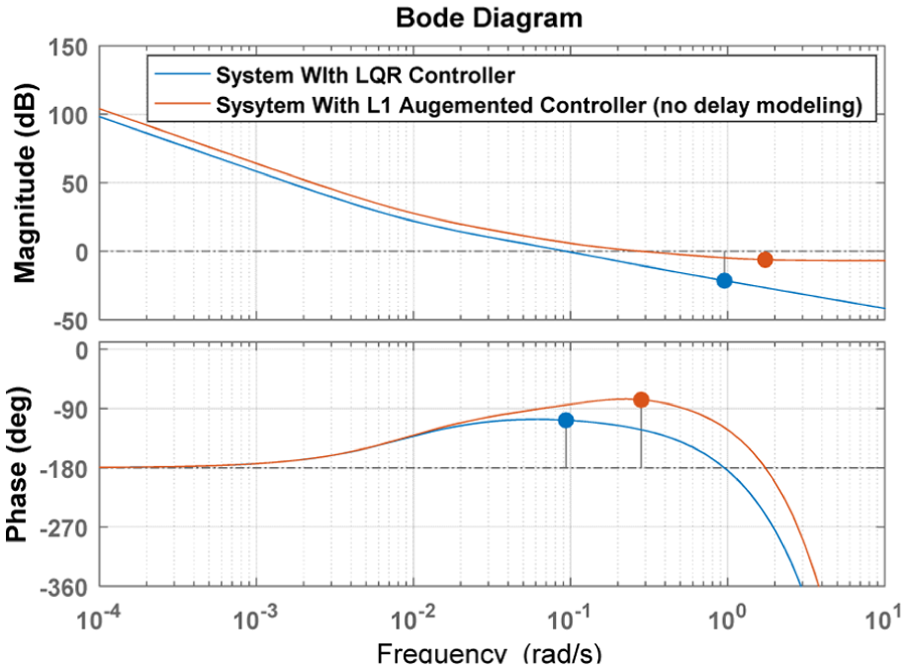
Bode plot for feedback system with LQR controller and L1 augmented controller.
It is seen that the L1 augmented controller has higher bandwidth and higher gain than the LQR baseline controller; this is why the performance of the L1 augmented controller is better than the LQR baseline controller in many simulation scenarios. But normally higher bandwidth may also mean reduction in robust stability margin and would introduce more noise or disturbance in closed-loop system. This can be seen in the controller output in some simulation cases.
Table 3 outlines the stability margin for the two feedback systems.
Stability margins in nominal condition.
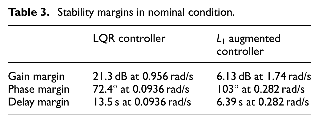
Since the nominal linear model already includes a delay of 1.6 s, the delay margins for the two controllers in the table are consistent with the designed delay margins of LQR and L1 adaptive controllers.
From the table, the stability margin for the L1 augmented controller is much smaller than the LQR controller, though the basic robustness is retained. When the time delay
When approximating the L1 adaptive output feedback controller with delay
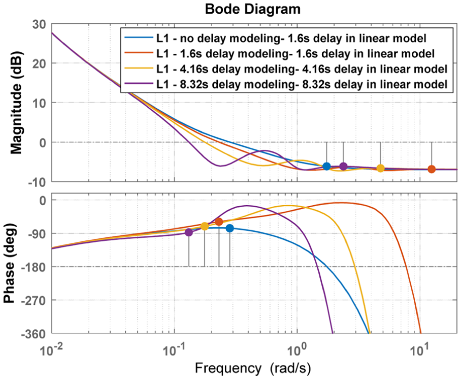
Bode plots for systems with different delays controlled by L1 augmented controller.
The TDMs for different delay cases in Figure 15 are listed in Table 4.
Stability margins for different delay cases.
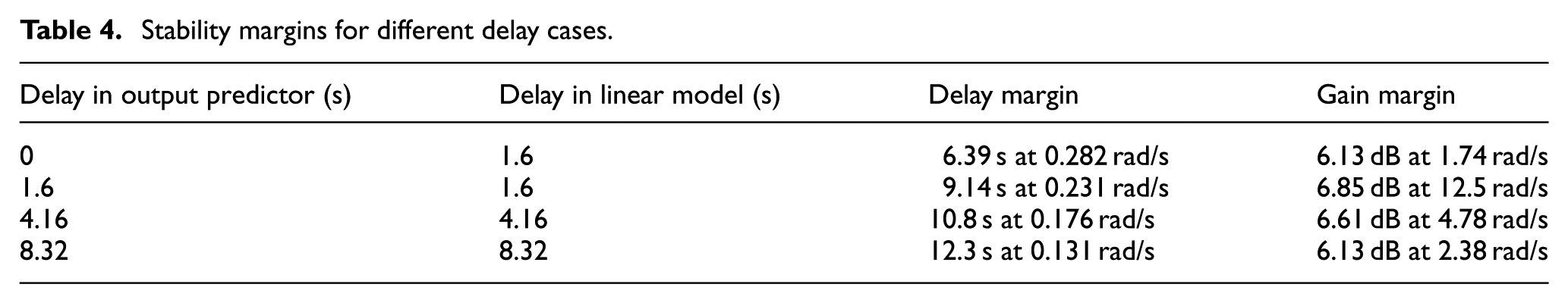
It is seen from Table 4 that with delay modeling in the output predictor, the L1 augment controller can assure higher extra TDM, in the condition that the delay is already presented in the linear temperature model. This property cannot be attained by the LQG controller alone. Thus, this design architecture improves the TDM considerably. This result is numerically verified in simulations. Of course, because of the existence of delay in the linear temperature model and the L1 adaptive controller, it is reasonable that the cross-frequency of the corresponding feedback systems would vary correspondingly, because the presence of delay would reduce the bandwidth of the feedback system. This feature is important for the temperature control in cryogenic wind tunnel, where the delay would always occur and vary over a range.
When the cryogenic wind tunnel is in operation, with the state variation of the wind tunnel, especially the Mach number, the delay will vary with these states and it could be estimated. The delay term in the output predictor incorporates some time-varying and nonlinear factor into the L1 adaptive controller architecture. With this feature, the L1 adaptive controller would adjust its bandwidth dynamically according to states of the wind tunnel. So, a dynamic trading off between the performance and robustness is realized through this design. It is obvious that this adjustment cannot occur in a very short period, otherwise complicated and unstable dynamics would occur.
Conclusion
The L1 augmented adaptive output feedback controller with modified piecewise constant adaptive law is applied to the temperature control of cryogenic wind tunnel. The modification of adaptive law plus the global nonlinear optimization of the filter in the L1 adaptive control architecture helps the controller achieve good control performance and acceptable robustness for the temperature control over a wide range of operations.
Simulations show that the LQG baseline controller and L1 augmented adaptive controller have better control performance compared with classical PI controller. Linear analysis show that the delay modeling in the output predictor greatly improves the TDM of the L1 augmented adaptive controller. The study and results here are encouraging and further application of L1 adaptive control to the entire cryogenic wind tunnel control could be warranted.
Footnotes
Appendix 1
Declaration of conflicting interests
The author(s) declared no potential conflicts of interest with respect to the research, authorship and/or publication of this article.
Funding
This work has been partially supported by the National Science and Technology Support Project, China (no. 2015BAF27B01)