Displacements of the pipe system caused by a transient phenomenon using the dynamic forces measured in the laboratory

Abstract

Background:

When transporting liquids, in particularly over long distances, dynamic forces in the system can present a risk. The larger the system size, and the greater the pressure, the more harmful the impact is of such forces. Water is transported in this way for domestic, industrial, and fire-fighting purposes. One of the impulses of dynamic force application may be the transition of the pressure wave in the water hammer.

Methods:

In this paper, the results of measured dynamic forces and associated displacements recorded on the model caused by transient flow conditions are presented. For measured forces, the displacements of the pipe were also calculated by using the oscillation motion equations. Force measurements and displacement analyses were carried out in laboratory on the model of a simple fire protection system equipped with three nozzles.

Results and Conclusions:

The measurement results and calculations were used to calibrate a mathematical model created using MATLAB software.

Introduction

A severe form of water hammer is called surge, which is a slow motion mass oscillation of water caused by internal pressure fluctuations in a system. ¹ This can be pictured as a slower “wave” of pressure arising within the system. If not controlled, it can yield the following results: damage to pipes, fittings, and valves, which in turn causes leaks and life shortening of the system. ²

In this paper is shown the use of equations describing the movement of suspended mass focused on the beam to calculate the displacement of the pipelines under the action of dynamic forces. This approach will allow to calculate, as far as possible, the actual displacement of the pipeline in the direction of flow change. This is very important information for designers calculating and selecting parameters of fixed points. ³

One of the factors that affect the reliability of an installation is its proper fastening to the structure of the building or other supporting components. This is especially important for installations which are exposed to dynamic loads. An example of an installation with the necessary high-reliability exposure to dynamic loads is a fire protection system. The selection of fastening elements for such an installation depends on the force that the fastener can carry. Unfortunately, it is usually assumed that the force is applied statically. Therefore, it is important to implement numerical models for the calculation of the displacements for the dynamic system and to compare them with physical models.

The measurements made allowed to calculate the parameters of the pipe-water system, which are necessary to calculate displacements based on the equation using the natural frequency for the entire system (i.e. the walls of the pipe and water filling the pipe). Such approach allows taking into account the impact on displacement not only the coefficient of elasticity of the pipe walls but also the bulk modulus of the water filling the pipe. Taking into account the mutual influence of both coefficients of elasticity (by calculating the natural frequency of oscillations) will allow a more accurate description of the phenomenon. The described problem does not finish solving the whole task. Currently, further research is planned to confirm the validity of the assumptions made, as well as to conduct measurements for pipes of various materials, with different wall thicknesses and the proportions of wall thickness and inside diameter, as well as for liquids with different densities. ⁴ Such an examination will allow for the development of a computational scheme, which in a simple way will allow, for example, engineers to calculate real ranges of displacements of pipe systems caused by transient phenomena. This knowledge, in turn, will allow adequate protection of pipe systems against damage, thanks to the appropriate pipe support selection.

The essence of the water hammer phenomenon

The disturbance that spreads in the form of a pressure wave occurs in transient fluid flow conditions. ⁵ The water hammer phenomenon happens when there are strong pressure oscillations in the pipe that is operating under pressure. ⁶ This is due to rapid changes in fluid flow rate forced in a short period of time. Physically, flows occurring in the form of hydraulic shock are caused by inertia of the mass of the fluid moving in the pipeline, where the flow rate changes suddenly. Rapid changes in the velocity and volume stream of flowing fluid leads to a local change in the proportion of kinetic and potential energy to the total energy of the section, which is expressed in a pressure increase or decrease in the stream. A rapid reduction of kinetic energy is observed in conditions of very rapid flow rate deceleration, which causes a sudden increase in potential energy, which in turn is manifested by a high-pressure increase. The course of water hammer phenomenon is significantly affected by fluid susceptibility to the compressibility and elasticity of the pipeline walls, that is, their sensitivity to elastic strains due to hydrodynamic pressure changes in the pipeline. In extreme cases, this sudden pressure increase may cause an excessive amount of critical tensile stress in the pipeline walls. ⁷

Water hammer is associated with an increase in pressure referred to as “positive impact,” which is accompanied by a sudden pressure drop called “negative impact.” The pressure gains for positive and negative water hammer phenomenon are calculated according to the formula of Joukowsky–Allievi

$$\mathrm{\Delta }p=\pm \rho c\mathrm{\Delta }v$$

(1)

where Δp is the maximum pipe pressure increase in water hammer phenomenon (F/L2], ρ is the fluid density (M/L3), c is the speed of propagation of the pressure wave, which is called celerity (L/T), and Δv is the change in velocity (L/T).

The dimensions are F (Force), L (Length), M (Mass), and T (Time).

For both positive and negative water hammer, two cases are possible:

• When t_z < T, where t_z is the time of total valve opening and T is the total time of wave propagation from the valve and back, then a straight surge will be observed in the pipe. When t_z > T, a non-straight surge will be noted in the pipe.

Contemporary analysis of water hammer phenomenon is most often based on the results obtained from the numerical solution of mathematical models. Most of these methods have their origin in differential equations of motion and continuity.

Differential equations of motion and continuity are adopted in a simplified form, that is, average flow parameters are “constant” and their derivatives are equal to zero, and the friction is reduced to a linear function. This results in a special solution of equations whose results are algebraic equations with respect to the parameters of pipelines and boundary conditions. Taking into account the impact of the enclosure on the solution, that is, a valve, pump, or change in pipe diameter, it is possible to achieve a solution, that is, a description of the phenomenon for a typical fluid transport system, without the necessity to refer to differential equations. It should be noted that by applying an equation reduced to a linear form to describe the phenomenon, the superposition principle can be used even for complex water supply or heating systems.

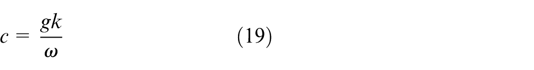
In the simplified equations of motion and continuity, pressure changes p are presented in the form of pressure head changes H = p/γ, and the equations have the following form ⁵

$$\frac{\partial H}{\partial x}+\frac{1}{\mathrm{gQ}}\frac{\partial Q}{\partial t}+\frac{\lambda Q^n}{2\mathrm{gD}{A}^n}=0$$

(2)

$$\frac{\partial Q}{\partial x}+\frac{\mathrm{gA}}{c^2}\frac{\partial H}{\partial t}=0$$

(3)

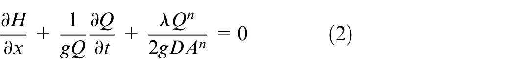
where H is the piezometric head (m) of the liquid column, Q is the volumetric flow rate (m3/s), λ is the multiplication factor of the friction element (–), n is the power exponent (–), D is the pipeline inner diameter (m), A is the pipeline cross-sectional area (m²), c is the celerity (m/s), and g is the acceleration due to gravity (m²/s).

Experimental facility in laboratory

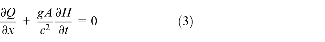
This paper presents and improves in detail the study which was simply presented in the article by Malesinska. ² The draft of the test stand concerned the simple scheme of a fire protection system, consisting only of the distribution pipe and one straight pipe (made up of three different diameters), armed with three nozzles. A simple geometric scheme allowed for an initial analysis and identification of phenomena accompanying the hydraulic shock wave propagation. The pipe system was designed in accordance with the applicable standards. A scheme of the designed installation is presented in Figure 1.

Figure 1.

Scheme of the laboratory test stand.

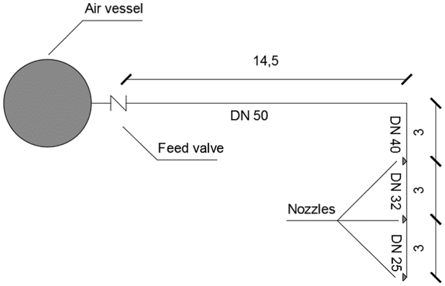
A system of steel of various outer diameters D₀ and wall thickness e was used in the experiment. The installation system that was accepted for the study was not filled with water. It was a model of an air system device used to protect the space of construction objects from the risk of frost or water evaporation. The installation system was equipped with three upright nozzles. The nozzles were placed one on each section of constant diameter DN40, DN32, and DN25 (Figure 2). The test stand for the water hammer analysis was constructed to perform the experiments, using the measuring system and recording of fast-changing pressure values.

Figure 2.

Upright nozzle installed in the pipe.

The model was supplied with water via a pressure increasing station (Figure 3). The water in the tank was refilled from a water supply system. Permanent steady flow conditions established in the model of the system were made possible by the use of a water–air tank which had a capacity of 300 dm3. The model was connected to the compressor, allowing an increase in the initial pressure in the system to the value of 5.5 bar (Figure 3).

Figure 3.

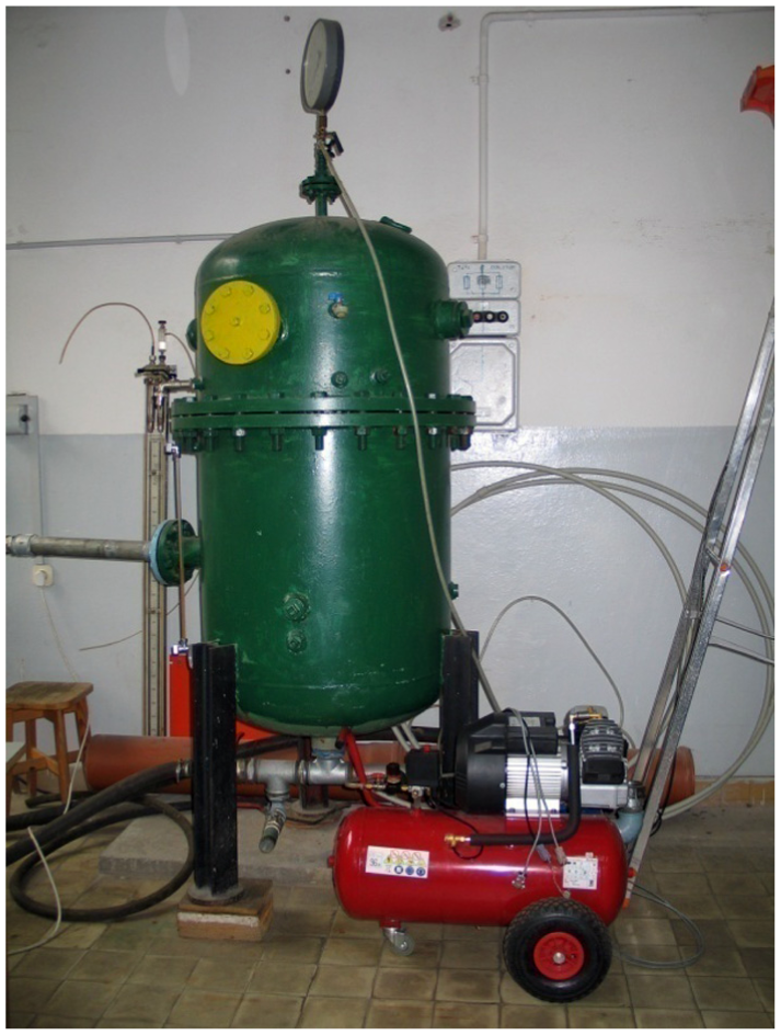
Pressure increasing station with the compressor.

The measurement and analysis of the results was for a simple water hammer only, that is,. with pressure wave transition time T always higher than the valve opening time t_z. The experiment was performed at an average temperature of 281 K.^8,9

The values of the forces impacting the components of the system were evaluated as follows:

1. In the first step, the forces were measured by a means of dynamometers (for a detailed description of the measurements and the results obtained, see Malesinska ² ). Figure 4 shows only the relationship between the measured forces and the pressure in the cross section in which the forces were measured.

2. Then, in the same section after removing the dynamometers, a fixed support was installed, constructed from a special clamp hung on an 80 cm threaded pipe (Figure 5). On this threaded pipe, after special preparation, a strain gauge was attached, which then allowed the stress measurements to take place (Figure 6). This fixed support is working as a cantilever beam with a point mass suspended at its end. The threaded pipe is considered as a cantilever beam and the steel pipe with water as a suspended mass.

Figure 4.

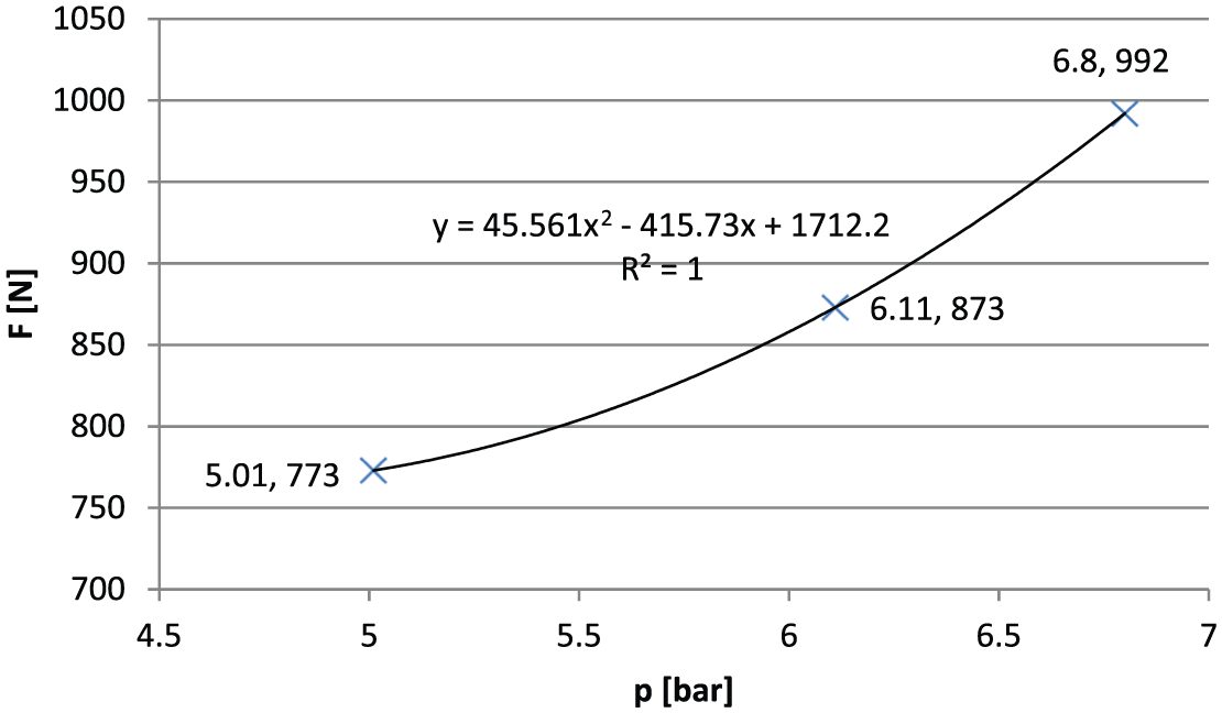
Relationship between the measured forces and the pressure in the cross section in which the forces were measured.

Figure 5.

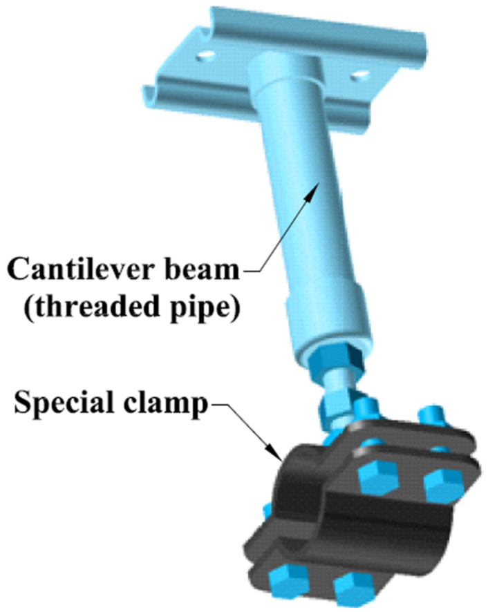
Scheme of a fixed support on which the model was suspended.

Figure 6.

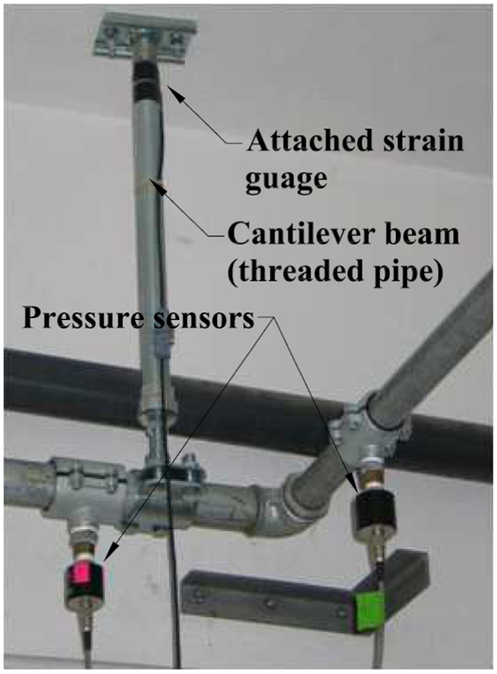
Fixed support with strain gauges attached.

In addition, measurement involved the concurrent measuring of pressures and flow rate and also the opening time of the feed valve. This measurement guaranteed a comparison of the water hammer phenomenon for the same (or very similar) boundary conditions. The valve opening time was closely linked to the valve opening angle. The measurement of voltage obtained from the potentiometer, mechanically coupled with the valve hand wheel, was used to register the changes during the opening angle of the feed valve. This procedure ensured a voltage proportional to the angle of rotation of the valve hand wheel. The turbine flow meter type TUV-1210, which could record the counted flow units, was used for flow measurement.

All the recorded values were recorded using a computer that was equipped with software that controlled the measurement process and all further processing. The basic software was developed in the “C” language, using “Turbo C” program for compilation and subroutine statements. Two versions of the software were designed: a version used to record the measurements and a version used to analyze the measurement results and the recorded value outputs.

Case study

The analysis included three work variants of the examined installation in the laboratory. Variant 1—one nozzle opened, variant 2—two nozzles opened, and variant 3—three nozzles opened.

Strain gauges installed on the cantilever beam of the fixed support allowed the calculation of the mass that was suspended on the beam, and then using the equation of oscillatory motion, the beam displacement was calculated for the suspended installation.

Before any measurements were taken, the strain gauges attached to the cantilever beam of the fixed support was calibrated, and the basic strength characteristic of the applied cantilever, which was necessary for calculation of the mass suspended on the beam, was determined.

Two wire strain gauges with the following parameters were attached to the beam:

• Nominal resistance R_nom = 600 Ω;

• Transformation constant K = 2.62;

• Active length l = 10 mm.

Both strain gauges were combined in a “half-bridge” system. The half-bridge system was used due to the measured parameter. In this system, one strain gauge was under compression and the other under tension. The strain gauges were attached to the previously prepared surface (the surface was leveled and cleaned). The place of attaching the strain gauges is shown in Figure 6. The strain gauges were attached as close as possible to the place where the beam was fastened, so as to minimize the effect of changing the length of the bent beam on the accuracy of strain gauge measurements. On the diagonal of the bridge to obtain the change in voltage ΔU, which depended on the resistance change ΔR/R

$$\frac{\mathrm{\Delta }U}{U}=\frac{1}{2}\frac{\mathrm{\Delta }R}{R}$$

(4)

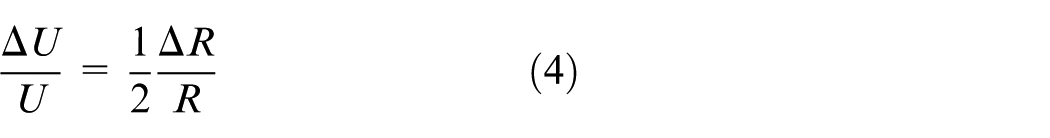
where U is the voltage of bridge powering (V)

$$\mathrm{\Delta }R=R_{\mathrm{nom}}K\epsilon$$

(5)

here, E is the relative elongation of strain gauges in the range of elastic strains and ε = 0.001, thus

$$\frac{\mathrm{\Delta }U}{U}=\frac{1}{2}\times 2.62\times 0.001=0.0013$$

(6)

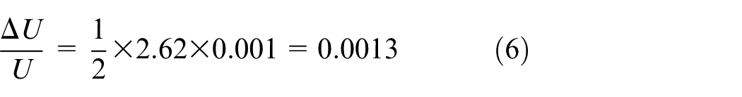
With the bridge powered by a voltage U of 5 V, a strain gauge bridge input signal imbalance is obtained and is equal to

$$\mathrm{\Delta }U=5\times 0.0013=0.0065\mathrm{V}=6.5\mathrm{mV}$$

(7)

By strengthening the direct current, having, for example, an amplification of L = 1000, it is possible to obtain an input signal of 6.5 V with 1 kN of force applied to the end of the cantilever beam in question.

Strain gauges calibrating was carried out by applying a force of known value (kN) and then reading the values of voltage (mV) corresponding to these known force values and their corresponding voltage changes. Since the relationship presented is linear, a best fit of the variability function was determined by the least squares method (Figure 7).

Figure 7.

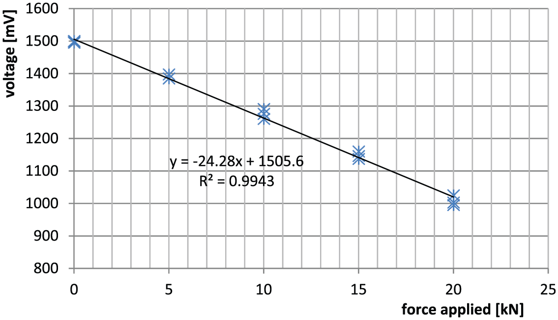
Strain gauges calibrating, readout of voltage value for known applied force value.

To calculate the strength parameters of the cantilever threaded pipe beam of the fixed support, it is necessary to know the basic geometrical and material parameters of the beam as follows:

• Inner diameter d = 33 mm;

• Outer diameter D = 39 mm (below the thread);

• Beam length L = 80 cm;

• Elastic modulus for steel E = 2.09 × 105 MPa.

Beam strength parameters were then calculated based on the above data values:

• Moment of inertia for beam cross section

$$J=\frac{\pi }{32}\left(D^4-d^4\right)=11.069{\mathrm{cm}}^4$$

(8)

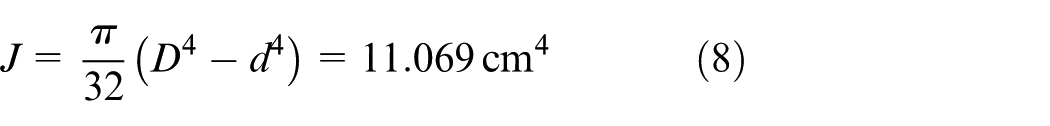
• Cross section modulus

$$W=\frac{\pi }{16}\left(\frac{D^4-d^4}{D}\right)=5.677{\mathrm{cm}}^3$$

(9)

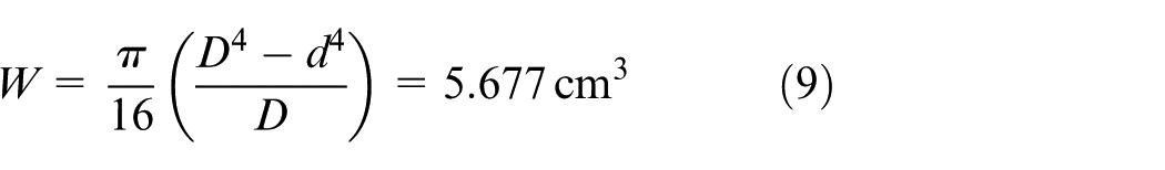
• Beam cross section

$$A=\frac{\pi }{4}(D^2-d^2)=3.39\mathrm{c}{\mathrm{m}}^2$$

(10)

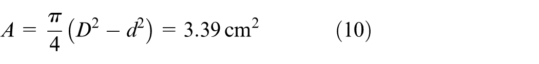
• With beam length of L = 80 cm, 271 cm³ of beam material net volume is obtained.

Calculation of the deflection of the cantilever beam—static force applied at the end of the cantilever

The displacement of the end of the beam as a result of the static action of the concentrated force, F, according to the material mechanics theory can be calculated from the relationship

$$f=\frac{F{L}^3}{3\mathrm{EJ}}$$

(11)

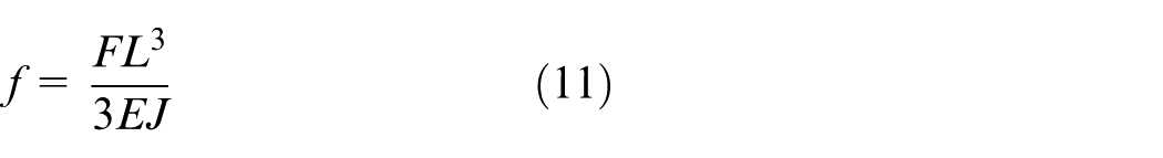
where f is the displacement of the end of the cantilever beam (deflection; m), F is the concentrated force (N), L is the beam length (m), E is the modulus of elasticity of the beam (Pa), and J is the modulus of inertia of the beam (m⁴).

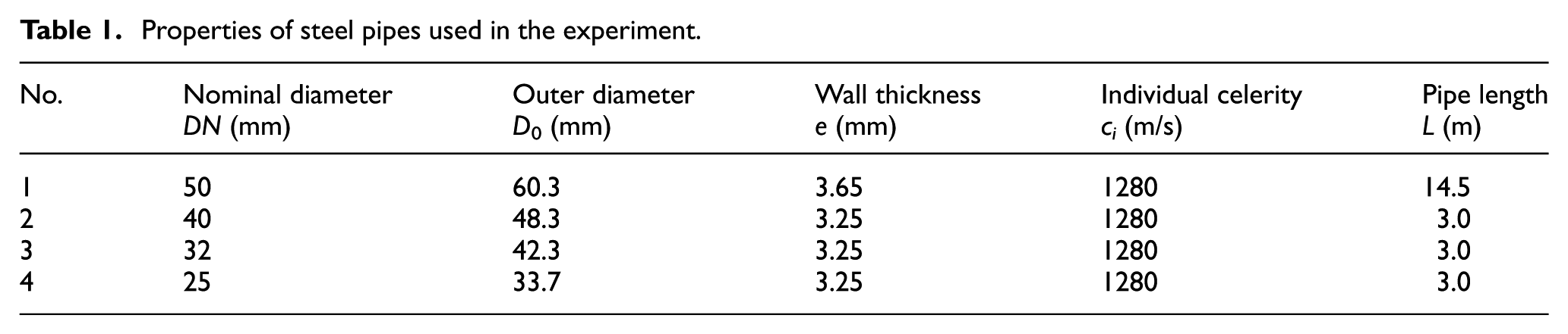
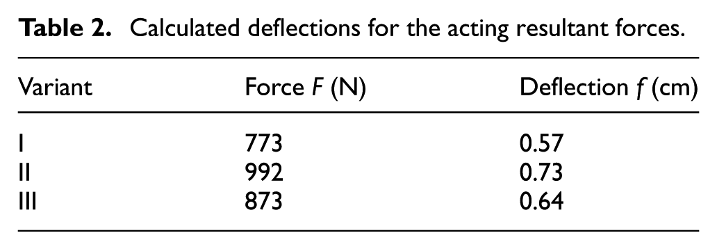
For the scheme presented in Figure 6, in the first stage of the test, the components of the force caused by the water hammer pressure wave were measured using dynamometers. ² The measured force components were used at this point to calculate the displacement of the beam end after the static force was applied at the end of the beam, that is, the threaded pipe of the fixed support. The cantilever beam was 80 cm long. For that particular beam length and the calculated strength parameters in Table 1, the deflection of the cantilever beam based on the calculated resultant forces was determined. The calculations are shown in Table 2.

Table 1.

Properties of steel pipes used in the experiment.

No.	Nominal diameter DN (mm)	Outer diameter D0 (mm)	Wall thickness e (mm)	Individual celerity ci (m/s)	Pipe length L (m)
1	50	60.3	3.65	1280	14.5
2	40	48.3	3.25	1280	3.0
3	32	42.3	3.25	1280	3.0
4	25	33.7	3.25	1280	3.0

Table 2.

Calculated deflections for the acting resultant forces.

Variant	Force F (N)	Deflection f (cm)
I	773	0.57
II	992	0.73
III	873	0.64

Use of the equation of the oscillatory motion for maximum deflection determination of the cantilever beam

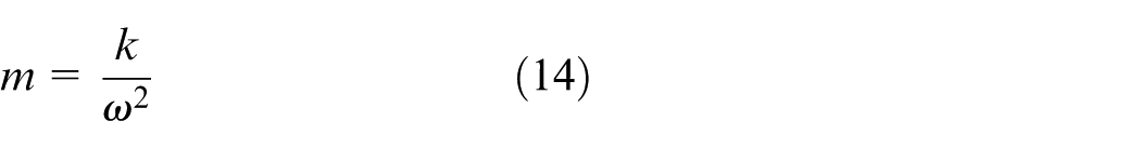
In the first step, the frequency of the natural oscillations of the pipe system not filled with water was measured in the laboratory. Oscillation inductions were forced by hitting with a soft pad. The oscillations constitute periodical motion in which all the points of the oscillating system, after a fixed time interval, would return to the initial value in a reproducible manner. This time interval is called the period of oscillation, and it is denoted by the letter T. The reciprocal of the period 1/T = f is called the frequency of oscillations. The frequency of natural oscillations of beam + mass f (Hz) system was measured, which gives

• Angle velocity

$$\omega =2\pi f(\mathrm{rad}/\mathrm{s})$$

(12)

• Angle velocity of beam with susceptibility k and mass concentrated at the end of the beam

$$\omega =\sqrt{\frac{k}{m}}$$

(13)

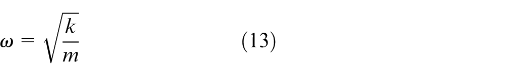
thus

$$m=\frac{k}{{\omega }^2}$$

(14)

in order to obtain the characteristic of oscillations, two records of suppressed oscillations, “dr1” and “dr2,” were made.

To register “dr1” (Figure 8), nine cycles took 1430 − 350 = 1080 recorded points (x and y = counted non-scaled impulses). Each registered point lasts 2 ms, thus 9 cycles lasted 2.16 s which corresponds to the following:

• Oscillation period T = 2.16/9 = 0.24 s;

• Oscillation frequency f = 4.17 Hz;

• Angle velocity ω₀ = 26.17 rad/s.

On the basis of the course of the forced oscillation for the empty pipe, “dr2,” similar to the first case “dr1,” 10 cycles were taken from the recorded characteristic, which took 1430 − 255 = 1175 registered points (x, y = counted non-scaled impulses) 2.35 s, corresponding to

• Oscillation period T = 2.35/10 = 0.235 s;

• Oscillation frequency f = 4.25 Hz;

• Angle velocity ω₀ = 26.72 rad/s.

Mean value of angle velocity for the dry system is ω_0avg = 26.45 rad/s.

Figure 8.

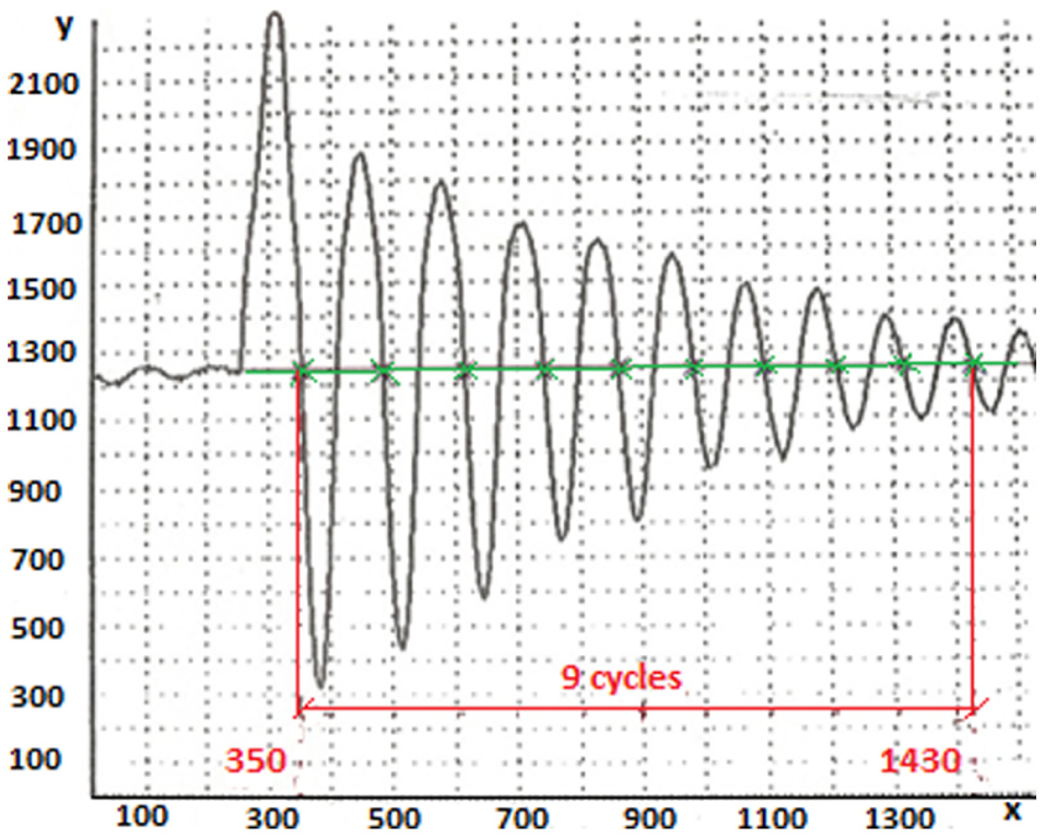
Course of forced oscillation for an empty pipe, “dr1.”

Finally, it is possible to calculate the mass suspended on the cantilever beam assuming that the suspension is at its end point. Hence, the constant of beam susceptibility was calculated from k = 3EJ/L3 (N/m), where L is the beam length. According to Equation (14), we know that $m=k/{\omega }^2$ , where k = 135 kN/m and ω = 26.45 rad/s are the values calculated for the examined system. Thus, we obtain mass value m = 193 kg.

In the same manner, using the measured characteristics, the following was established for the wet pipes:

• Oscillation period T = 0.28 s;

• Oscillation frequency f = 3.57 Hz;

• Angle velocity ω = 22.4 rad/s, calculated from Equation (12);

• Mass m = 269 kg, calculated from Equation (14).

As the value of the concentrated mass suspended at the end of the cantilever beam is known, it was possible to analyze the oscillations forced by a sudden application of force—a response of the system to the pressure wave propagation. Forcing the oscillating system motion is a certain process, and as known, its nature can be of an aperiodic process character, in particular the transition one.

Then, the mathematical model of the system with suppressing takes the following form

$$m\stackrel{··}{x}+c\stackrel{·}{x}+\mathrm{kx}=F\left(t\right)$$

(15)

where force F(t) may be aperiodic and also a discontinuous function. To determine the motion of the oscillating system affected by the action of aperiodic extortions, the response of the system on two elementary forces can be analyzed, that is, the unit impulse and the unit step. The impulse is a measure of the impact of short-term forces, for example, the closing and quick opening of the feeding valve. The step is a response to the force of the constant value suddenly applied to the physical system, for example, a heat shock caused by a sudden temperature change.

In the case of the water hammer phenomenon, we are dealing with an applied instantaneous force. A measure of the impact of short-term forces is impulse S, that is

$$S=\underset{t_1}{\overset{t_2}{\int }}F\left(t\right)\mathrm{dt}$$

(16)

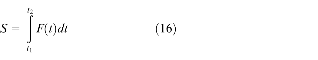
When the time Δt of force F(t) operation is very short, as it is in the case of pressure wave propagation, it is an instantaneous force. The solution of the equation of suppressed oscillatory motion induced by instantaneous force, taking into account the subcritical suppression, is the following function

$$x\left(t\right)=\frac{s}{m{\omega }_D}{e}^{-\mathrm{bt}}\sin {\omega }_{D}t$$

(17)

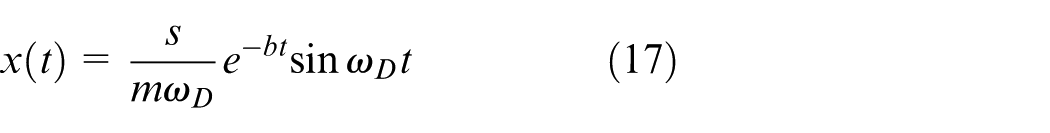
where x is the displacement of the end of the cantilever beam in time; S is the impulse caused by instantaneous force action, S = F₀Δt; m is the mass, in this case calculated based on measured characteristics of mass value for a wet installation, m = 269 kg; and ω_D is the frequency of suppressed free oscillations (natural frequency)

$${\omega }_D=\sqrt{{\omega }_0^2-b^2}$$

(18)

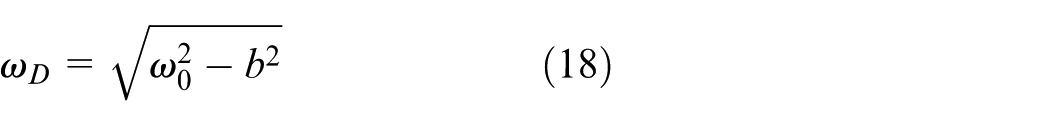
ω₀ is the natural oscillations frequency; b is the normalized suppression coefficient, b = c/2 m; and c is the viscous suppression coefficient related to the suppressive properties of viscoelastic material

$$c=\frac{\mathrm{gk}}{\omega }$$

(19)

$$\omega ={\omega }_0$$

(20)

g is the number characterizing the suppression properties of the beam

$$g=\frac{\mathrm{Im}{E}^{*}}{\mathrm{Re}{E}^{*}}$$

(21)

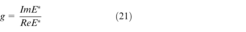
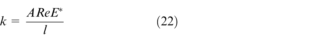
ImE is the imaginary part of complex elastic modulus, ReE is the real part of complex elastic modulus, E is the complex elastic modulus, that is, variable over time, and k is the number characterizing elastic properties of the beam

$$k=\frac{\mathrm{ARe}{E}^{*}}{l}$$

(22)

On the basis of the experiments conducted, and by calculating certain value characteristic of the analyzed system, it is possible to derive an equation of suppressed oscillatory motion caused by the activity of the instantaneous force–pressure wave propagation.

In order to derive an equation of suppressed oscillatory motion, the relationship for T_D may be used, which is defined as the time interval between two successive peaks in the same direction. The T_D value is constant in time and can be calculated from the following relationship

$$T_D=\frac{2\pi }{\sqrt{{\omega }_0^2-b^2}}$$

(23)

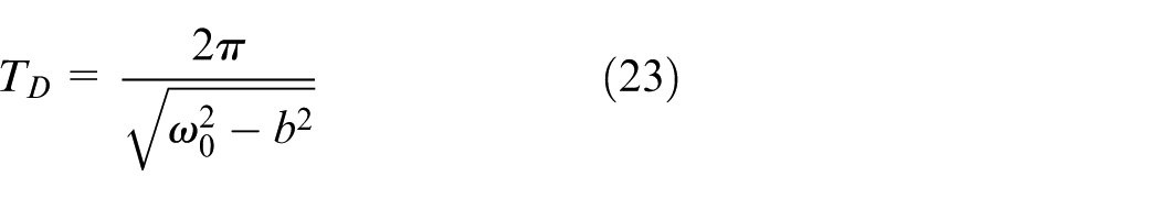
Explanations are similar to those in Equation (18). Having the measured characteristics for the experiment, it is now possible to determine the value of T_D = 0.29 s. After converting the above relationship, it is possible to calculate the standardized suppression coefficient b = 5.69 rad/s and ω_D = 21.66 rad/s.

For the assumed unit impulse inducing system oscillation, the equation of the change of displacement versus time takes the form (h and x are the same parameters describing displacement of the end of the cantilever beam)

$$h\left(t\right)=\frac{1}{m{\omega }_D}{e}^{-\mathrm{bt}}\sin {\omega }_{D}t$$

(24)

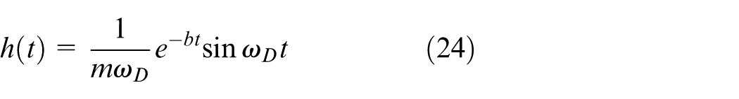
m = 269 kg, b = 5.69 rad/s, ω_D = 21.66 rad/s, and T_D = 0.29 s

$$h\left(t\right)=1.716\times {10}^{-4}{e}^{-5.69t}\sin 21.66t$$

(25)

In the case of a water hammer, it was assumed that the concentrated force F was acting in infinite time. So, it is assumed that the impulse S is equal to the force F.

According to the equation of the oscillatory motion, the maximum displacement x_max is as follows

$$x_{\max }=\frac{S}{m{\omega }_D}{e}^{\frac{-b\pi }{2{\omega }_D}}\mathrm{for}t=\frac{\pi }{2{\omega }_D}=0.07\mathrm{s}$$

(26)

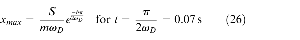
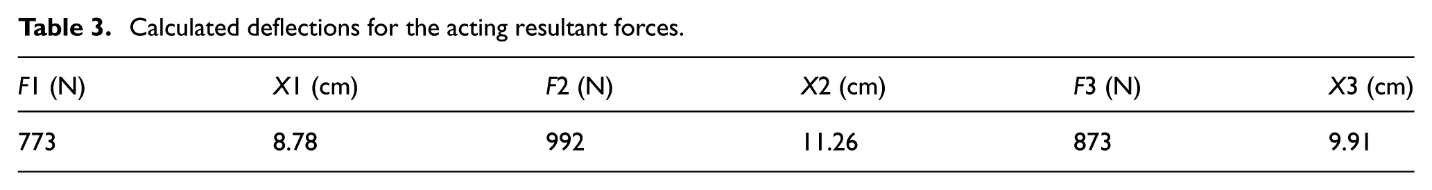
Assuming S = F, x_max was calculated for the force values listed in Table 3.

Table 3.

Calculated deflections for the acting resultant forces.

F1 (N)	X1 (cm)	F2 (N)	X2 (cm)	F3 (N)	X3 (cm)
773	8.78	992	11.26	873	9.91

Knowing the function describing end of the cantilever beam displacement, the pipe of the installation displacement is known as well.

MATLAB package implementation

To calculate the change in displacement of the end of the supporting beam for unit impulse versus time, the MATLAB package was used. For this purpose, the following oscillation function was created:

function [x, t] = oscillation (S, m, omega0, Td, and figure), which requires the following input parameters:

S is the value of unit impulse (N), m is the mass concentrated at the end of beam (kg), omega0 is the angular velocity (rad/s), Td is the contractual period (s), and figure is the parameter specifying whether to create a figure or not.

The function returns two output values: x is the value of maximum displacement (cm) and t is the time, after which the value of maximum displacement occurred.

To solve the problem, all of the values needed for Equation (26) must be calculated. Based on the ω₀ and T_d parameters, the value of the normalized suppression coefficient (b) is determined. Then, by using this value, the value of ω_D is calculated. After calculating all the necessary values, the symbolic variable t is created, and Equation (26) is built using the provided and calculated values.

The built equation is solved to find the global minimum using the GlobalSearch class and the corresponding settings for the optimization problem of one variable. ¹⁰

Finally, the graph of the function is plotted, and the maximum value found (the minimum value determined by the above optimization problem) is marked on the graph, and the two output parameters are returned from the function. The function block diagram is shown in Figure 9 (the following is an example of a function call).

Figure 9.

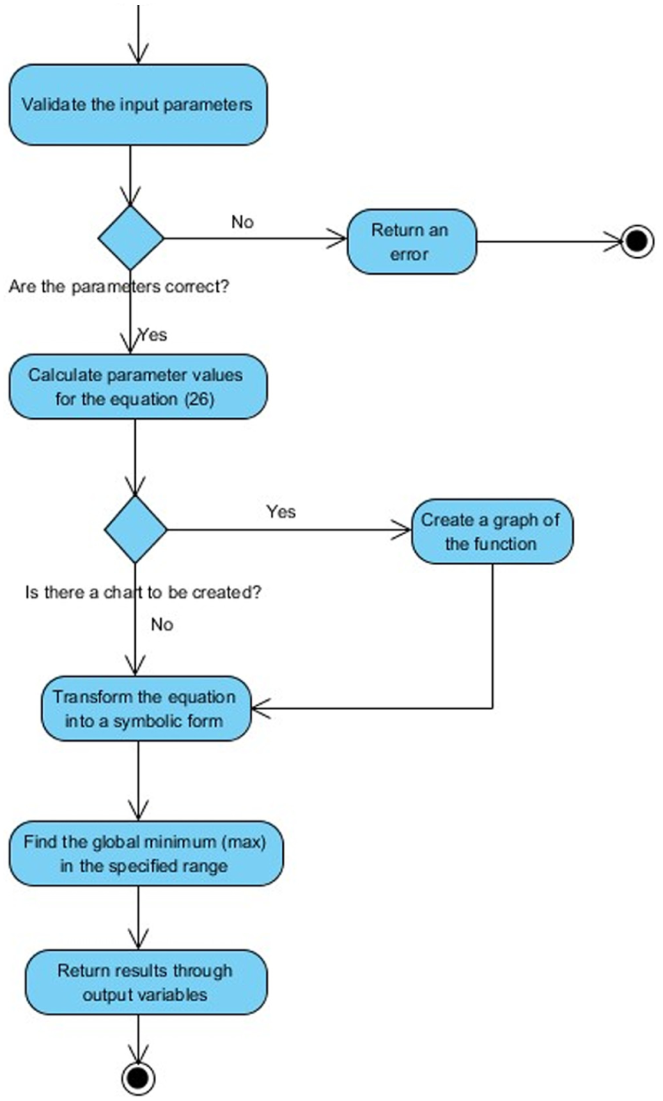
Function block diagram.

For the input parameters S = 992 N, m = 269 kg, ω₀ = 22.4 rad/s, and T_d = 0.29 s, output parameters were obtained: x = 11.661 cm and t = 0.060653 s, and the graph of the function was as shown in Figure 10.

Figure 10.

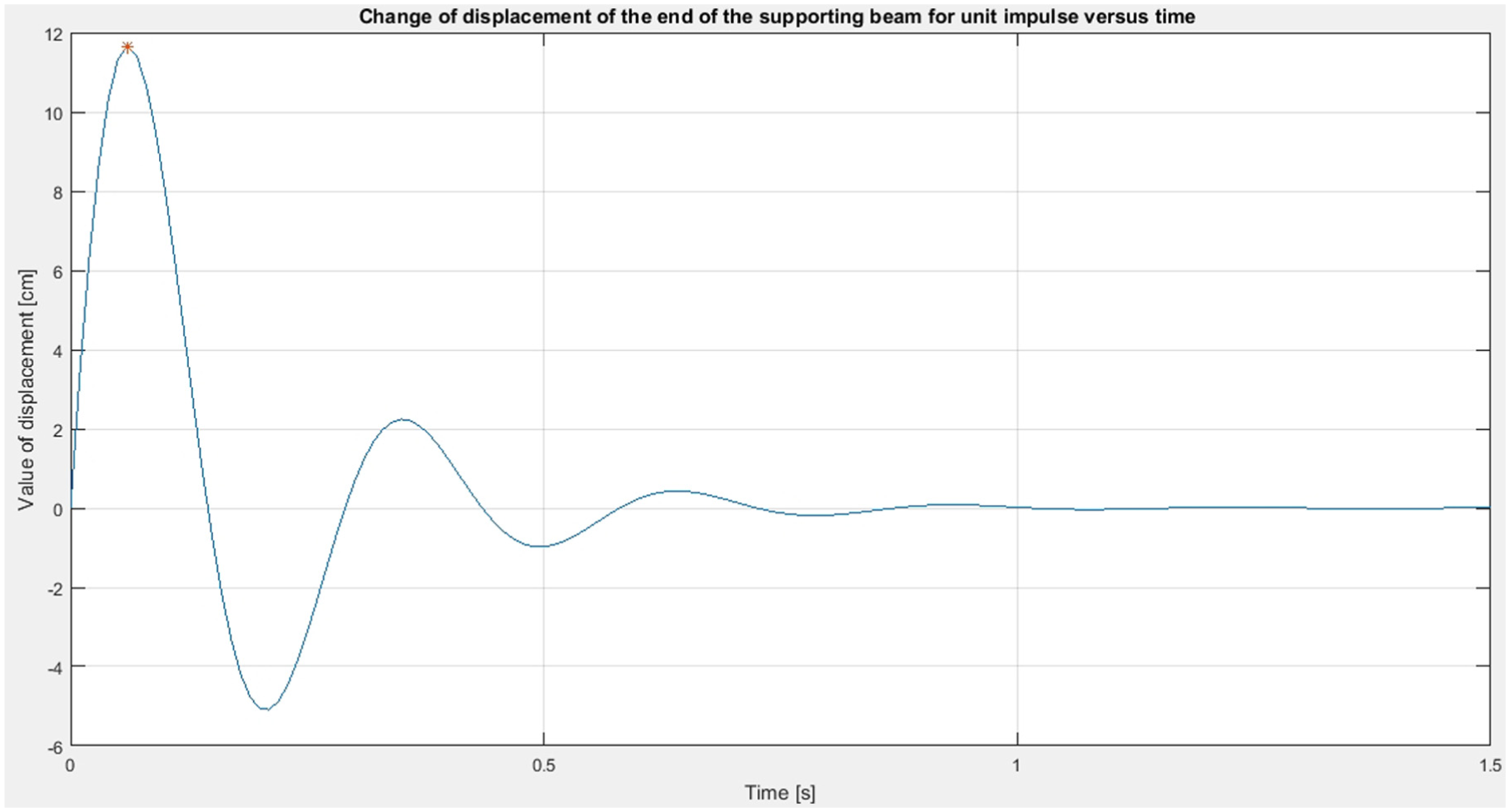
Change in displacement for unit impulse versus time.

Summary

One of the factors affecting the reliability of an installation is its proper suspension to the structure of the building or other supporting components. This is especially important for installations which are exposed to dynamic loads. An example of an installation with the required high reliability exposed to dynamic loads is a fire protection system. The selection of fastening elements for a given type of installation depends on the force that the fastener can carry. Unfortunately, it is usually assumed that the force is applied statically. This article presents the values of installation displacement calculated traditionally for the static system (f). These values were compared with the displacements obtained with the use of the oscillation equation (x or h). Such calculations were possible thanks to the results of research conducted on a physical model in the laboratory. It was not possible to measure displacements at this stage of the research. Installed strain gauges were used to measure the quantities necessary to determine the natural frequency of the system. The displacement values obtained from the oscillation equation were on average 10 times larger than the displacements calculated from the static system. ¹¹ The order of magnitude of the displacements calculated on the basis of the oscillation motion theory was consistent with the eye observations carried out directly on the model during the measurements. The next stage of the research will be the recording of the displacements of the system by means of a camera with software for the recording of fast-changing phenomena. This will allow the getting of real displacement functions and validation of the use of equations of oscillation motion (taking into account the natural frequency of the system) for the description of the phenomenon, assuming S = F. The obtained measurement results will allow for a possible correction of the equations used. Based on current knowledge, it is well known that the coefficient of compressibility (inverse of the bulk modulus) of a liquid is meaningful when analyzing a water hammer phenomenon. However, from the material mechanics point of view, the bulk modulus of the liquid is negligibly small (e.g. 2.2 GPa for water compared to 160 GPa for steel). Nevertheless, according to the authors, the bulk modulus of the liquid together with the coefficient of elasticity of the pipe walls has an influence on the suppression rate and thus on the size of displacements caused by transient phenomena.